Relaxation properties in classical diamagnetism

Abstract

In the present paper the problem of the relaxation of magnetization to equilibrium (i.e., with no magnetization) is investigated numerically for a variant of the well–known model introduced by Bohr to study the diamagnetism of electrons in metals. Such a model is mathematically equivalent to a billiard with obstacles in a magnetic field. We show that it is not guaranteed that equilibrium is attained within the typical time scales of microscopic dynamics. Indeed, considering an out of equilibrium state produced by an adiabatic switching on of a magnetic field, we show that, depending on the values of the parameters, one has a relaxation either to equilibrium or to a diamagnetic (presumably metastable) state. The analogy with the relaxation properties in the FPU problem is also pointed out.

PACS numbers: 75.20.–g, 05.45.Pq

Running title: classical diamagnetic properties of matter

1 Introduction

It is well known (see Refs. [1, 2]) that, according to classical statistical mechanics, at equilibrium matter doesn’t exhibit any diamagnetic effects. For a classical model of free electrons in metals this was first stated by Bohr (see [3]). Indeed, he pointed out that the Maxwell–Boltzmann distribution of the electron velocities depends, at a fixed temperature, only on the system’s energy. On the other hand, the value of energy does not depend on the magnetic field. So the electron velocity distribution, being unaffected by the magnetic field, is the same as in the case of a vanishing field, and thus magnetization vanishes. The same line of reasoning is followed in the general case; see for example the classical textbook by Feynman [4].

On the other hand, a magnetization can exist in an out of equilibrium state, as typically occurs when a magnetic field is switched on, because this induces an electric field which does perform some work on the system. In the very words of Bohr (see Ref. [3], page 382): “It must be pointed out, however, that in a piece of metal exposed to a variable magnetic field there will arise a collective motion of the electrons – the so called Foucault current – produced by the electric field which, according to the electromagnetic theory, is inextricably connected with the variation of the magnetic field; this current will produce a magnetic effect that will counteract the variation of the magnetic field…”. Bohr, however, also added “…the induced collective motion of the electrons will disappear very rapidly after the magnetic field has become constant, without leaving any permanent effect upon the statistical distribution of the velocities of the electrons”. In other words, a magnetization is induced by the switching on of the field, but it will disappear when the system will have relaxed to the final equilibrium. In addition, Bohr guessed that the relaxation should always be rapid. In the present paper we perform some numerical computations in order to check whether this is actually the case. We will show that there are cases in which, even in systems as billiards (which may be very chaotic, see [5, 6]), there appear several time scales for the relaxation to equilibrium. In some cases the equilibrium is not even attained within the available simulation time, analogously to what occurs in FPU systems.

The existence of a relaxation time to equilibrium for magnetization is of particular importance because, if one performs measurements on a time scale shorter than that needed to reach equilibrium, an effective nonvanishing magnetization will show up. In particular, if the system remains frozen in some metastable state, this diamagnetic property may be mistaken for a true equilibrium one. In any case, the system will then actually present some “effective” diamagnetic property, notwithstanding the fact that magnetization vanishes at equilibrium. The situation is reminiscent of that of FPU systems (see Refs. [7, 8, 9]), where the lack of thermalization leads to values of the specific heat smaller than the equilibrium one. So the question is the following one: if initially (when the magnetic field vanishes) the system is distributed according the to Gibbs statistics, and then a magnetic field is “slowly” increased up to a final value $\mathbf{B}_{0}$, how much time is it necessary for the system to reach a state in which the magnetization vanishes again?

The problem of the rate of thermalization for magnetization will be dealt with in this paper through numerical computations, making reference to a variant of the well–known Bohr model for free electrons in metals, which will be described in a moment. We will consider a system of $N$ electrons and compute numerically their trajectories, so that the total magnetization (which, we recall, is proportional to the total angular momentum) can be evaluated at any time.

The macroscopic magnetization should in principle be defined through a Gibbs average over the initial data in phase space. However, in the present paper we will take a more pragmatic approach, and will define the macroscopic magnetization through a “moving average” of the “instantaneous” total magnetization over a fixed time interval for a single orbit, as will be explained more precisely later. The aim is to study the behaviour of magnetization as time increases, and in particular to see whether it vanishes, or rather it settles down to some constant value.

We first consider the original Bohr model, i.e., a set of noninteracting electrons moving on a plane normal to the magnetic field $\mathbf{B}$, and confined in a domain of a simple shape (in particular we consider circular domains). The numerical simulations show that, after the field has been switched on, in this model there is no relaxation at all, so that one ends up with a perpetual nonvanishing magnetization.

Thus, we modify the model and insert inside the domain some fixed obstacles simulating the interaction of the electrons with the ionic lattice of a metal, so that we end up with a dynamical system which is just a billiard in a magnetic field. Systems of this type are well studied in the literature (see for example [10, 11, 12, 13]), with the aim of determining how do their ergodic properties depend on the magnetic field. At variance with the quoted papers, however, we deal here with a time–dependent magnetic field, just because we are interested in studying the effects of an adiabatic switching on of the field, which produces a nonequilibrium state of magnetization. We find that, in the modified Bohr model, after the field was switched on indeed in general one can have relaxation to equilibrium or to a metaequilibrium state according to the values of the parameters.

The paper is organized as follows. In Section 2 we define the model, and briefly discuss the numerical method for integrating the equations of motion. We also check that, in the case of a constant $\mathbf{B}$, the magnetization vanishes, in agreement with Bohr’s theorem. In Section 3 we discuss the case in which the magnetic field $\mathbf{B}$ is switched on adiabatically, and illustrate the main result of the paper, namely that situations of apparent metastability may occur. In Section 4 the results are discussed. In an Appendix we recall how, according to Linear Response Theory, the diamagnetic susceptibility is related to the time–autocorrelation of magnetization.

2 The model

The model concerns a system of $N$ identical point particles of mass $m$ and charge $q$, moving in a plane. We denote by $\mathbf{x}_{i}=(x^{(i)},y^{(i)})$, $i=1,\ldots,N$, the coordinates of the $i$–th particle and by $\mathbf{p}_{i}=(p_{x}^{(i)},p_{y}^{(i)})$ their conjugate momenta. The magnetic field is taken perpendicular to the plane and homogeneous, i.e., one has $\mathbf{B}=(0,0,B(t))$, so that the vector potential $\mathbf{A}$ at point $\mathbf{r}$ is given by $\mathbf{A}(\mathbf{r})=\frac{1}{2}\mathbf{B}\wedge\mathbf{r}$, where $\wedge$ denotes the vector product. The particles do not interact with each other, and the Hamiltonian is simply given by

$$H(\mathbf{p}_{i},\mathbf{x}_{i},t)=\frac{1}{2m}\sum_{i=1}^{N}\Big{(}\mathbf{p}_{i}-\frac{q}{2c}\mathbf{B}(t)\wedge\mathbf{x}_{i}\Big{)}^{2}+\sum_{i=1}^{N}V(\mathbf{x}_{i})\ ,$$ (1)

where $c$ is the speed of light, while $V(\mathbf{r})$ is a confining potential, i.e. a function vanishing inside the allowed domain and diverging outside it (corresponding to a boundary condition of elastic reflection). We take for $m$ and $q$ the mass and the charge of the electron, and we use atomic units, in which the electron mass, the electron charge and the reduced Planck constant $\hbar$ are all set equal to 1. The number $N$ of particles in most simulations is taken in the range $10^{3}\div 10^{4}$, and in some cases is increased up to $10^{5}$.

The time dependence of the magnetic field is taken as

$$\mathbf{B}(t)=\frac{\mathbf{B}_{0}}{2}\Big{(}1+\tanh\frac{t-t_{i}}{t_{c}}\Big{)}\ ,$$ (2)

where $t_{c}$ is the characteristic time over which the magnetic field varies, and $t_{i}$ is, in a sense, the time at which the field is switched on. Indeed, for times $t-t_{i}<-5t_{c}$ the magnetic field essentially vanishes, while for $t-t_{i}>5t_{c}$ the field is essentially constant, equal to $\mathbf{B}_{0}$. The values of the magnetic field $B_{0}=|\mathbf{B}_{0}|$ are taken in the range $10^{-3}\div 10^{-2}$ (in atomic units), while $t_{c}$ is taken of order $10^{6}$ (in our time unit) and $t_{i}$ of the order $5\;10^{7}$. For what concerns the domain, we take it of two different kinds: the first one is a “simple domain”, i.e. a circular domain of radius $R$, with $R$ in the range $5\times 10^{3}\div 5\times 10^{4}$ (expressed in atomic units, i.e. the Bohr radius). We will show in the next Section that for this type of domain the model shows no relaxation at all.

The second type of domain is chosen in order to describe a more realistic situation, in which the electrons interact with the ionic lattice of a metal. Thus, we add inside the circular domain a square lattice of circular obstacles. The radius $R$ of the circle is taken fixed equal to $5\times 10^{4}$, while the radius $r$ of each obstacle is taken equal to $10$, and the lattice step in the range from $10^{3}$ to $10^{4}$.

From Hamiltonian (1) one gets the equations of motion, which are all decoupled because the particles have no mutual interaction. Such equations are numerically integrated using the “leap frog” algorithm which we now briefly describe. The integration step of the “leap frog” method from the values $\mathbf{p}_{i},\mathbf{x}_{i}$ at time $t$ to the values $\mathbf{p}^{\prime}_{i},\mathbf{x}^{\prime}_{i}$ at time $t+\tau$ is performed by a canonical transformation with generating function

$$S=\sum_{i=1}^{N}\mathbf{p}_{i}\cdot\mathbf{x}^{\prime}_{i}-\tau H(\mathbf{p}_{i},\mathbf{x}^{\prime}_{i},t+\tau)\ .$$ (3)

This gives an implicit integration scheme, which can be easily made explicit for the particular form of our Hamiltonian (1).

The collision with the boundary is dealt with in the following way: one performs an integration step and then checks whether the particle remains inside the allowed domain. If this is not the case, the evolution is made not according to the leap frog algorithm, but as follows: the position $\mathbf{x}_{i}$ and the component of $\mathbf{p}_{i}$ tangent to the boundary are left unchanged, while the normal component of the momentum $\mathbf{p}_{i}$ changes its sign. One checks that this approximation is sufficient to keep constant the energy of the system.

Finally, the initial data are taken at random in the following way: the initial positions of the particles are uniformly distributed inside the allowed domain, while the initial velocities are distributed according to a Maxwell–Boltzmann distribution at a temperature $T$. We take a temperature $T$ such that $k_{B}T=1/250$ in our units ($k_{B}$ being the Boltzmann constant). This temperature corresponds to a mean velocity approximately equal to $1/3000$ the speed of light, which is a typical velocity of the electrons in metals at ordinary conditions (see [14]).

We now explain how the magnetization $\mathbf{M}$ is computed. The instantaneous value of magnetization, let us call it $\mathfrak{M}$, is given by

$$\mathfrak{M}=\frac{q}{2c}\sum_{i=1}^{N}\mathbf{x}_{i}\wedge\dot{\mathbf{x}}_{i}\equiv\frac{q}{2mc}\mathbf{L}_{tot}\ ,$$ (4)

where $\mathbf{L}_{tot}$ is the total angular momentum. Such a quantity is found to exhibit, in our numerical computations, some fluctuations. So, in order to smooth them out, we perform a moving average, i.e., we report, in place of the instantaneous values, the corresponding time averages over a small time interval (of the order of one hundredth of the total integration time).

Figure 1: Plot of the component of $\mathbf{M}(t)$ along the field $\mathbf{B}$ versus time in the original Bohr model, for three different samples of 10³ electrons. The magnetic field is equal to 0.001.

Some examples of the results of this procedure are shown in Figure 1, which refers to the case $|\mathbf{B}|=0.001$ independent of time, and to three different samples of $N=1000$ electrons each. At first sight it appears that for each sample the magnetization is constant and different from zero. This actually is a statistical effect due to the finiteness of the system (1000 electrons). Indeed, as pointed out by Bohr, the value of magnetization turns out to be due to the contributions of two populations. The first one is the population of the bulk electrons, which stay deep inside the domain without hitting the boundary. They move in circles, producing a magnetic field which is directed against the external one.

The second population is made of electrons which repeatedly hit the boundary and produce a current directed opposite to that of the first population. The two contributions would exactly cancel each other in the limit of an infinite number of electrons. This was the conclusion of Bohr.

In our simulations the populations are finite, so that the two contributions are slightly different. To evaluate this statistical effect we perform ten different simulations (with $B=0.01$ and $N=10^{5}$); in five cases we take into account the contribution of the boundary, while in the remaining ones we eliminate the boundary, i.e. we just put $V\buildrel{\rm def}\over{=}0$ into Hamiltonian (1). The mean and the standard deviation (over the samples) of the magnetization per electron $|\mathbf{M}|/N$ for the cases cases are reported in Table 1.

Table 1: Magnetization per electron in the case of a constant field (without obstacles), in the presence or in the absence of the boundary. The magnetic field is taken equal to 0.01, the radius of the circle is taken equal to $5000$, the number of electrons is taken equal to 10⁵.

	mean	standard deviation
with boundary	-0.0007	0.0024
without boundary	-0.3994	0.0022

As one sees, in the absence of the boundary the magnetization per electron turns out to be finite. This fact, by the way, was already pointed out in a recent paper (see [15]). Instead, when the boundary is present (first line of Table 1), the results are consistent with a vanishing magnetization, as predicted by Bohr.

Things are however different if one considers a time–dependent magnetic field, as occurs when the field is adiabatic switched on. This is discussed in the next Section.

3 The case of a time–dependent field

The first result in the presence of a time–dependent field is summarized in Figure 2, which refers to the original Bohr model, i.e., the case of a circular domain without obstacles. We see that in this case there is no relaxation at all to a vanishing magnetization, so that the model exhibits a fully diamagnetic behaviour. The reason is apparent from inspection of Figure 3, in which the positions of the electrons at the end of the same simulation considered in Figure 2, are shown. Indeed, one sees that the electrons are no more uniformly distributed in the available domain, but are instead concentrated away from the boundary. This corresponds to the appearance of a magnetic pressure which confines the electrons away from the boundary, analogously to what occurs in the magnetic confinement in Tokamaks.

Figure 2: Plot of the component of $\mathbf{M}(t)$ along the field $\mathbf{B}$ versus time, for a circular domain of radius 5000 and no obstacles, with a magnetic field adiabatically switched on with a characteristic time equal to $5\times 10^{6}$. The number of electrons is 5000, and the final field strength is 0.01.

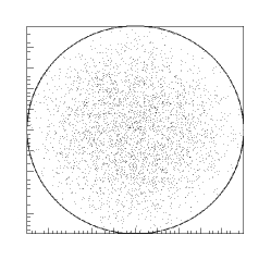
Figure 3: Plot of the positions of the electrons at the end of the simulation considered in Figure 2.

Thus, the contribution to magnetization due to the “bulk” electrons and that due to those hitting the boundary become different, the Bohr compensation does not occur anymore, and the magnetization turns out to be different from zero. This shows that, in order to obtain a classical diamagnetic effect, it is not necessary to physically eliminate the border from the model (as was done in Ref. [15] for a case of a constant field), because a diamagnetic effect already manifests itself even in the presence of the border, just as a consequence of the adiabatic switching on of the field.

From a mathematical point of view, the appearance of a magnetization is due to the fact that, in the case of a circular domain, the total angular momentum is conserved once the magnetic field becomes static.

Figure 4: Plot of the component of $\mathbf{M}(t)$ along the field $\mathbf{B}$ versus time in the case of a circular domains and a lattice of obstacles. The field strength is equal to $0.001$, the switching time $t_{c}$ is equal to $5\times 10^{6}$ and the number of electrons is $N=2500$. Upper panel: distance between obstacles equal to 2500. Lower panel: distance between obstacles equal to 4500.

However, in a more realistic model of electron conduction in a metal, the total angular momentum of the electrons alone would not be conserved, because of the scattering of the electrons by the ions (electron–phonon interaction), although the total angular momentum is obviously still conserved. In order to mimic the ionic lattice of a metal, we change the shape of the domain, by inserting a square lattice of circular obstacles. Thus, the total angular momentum of the electrons is no more conserved. We first checked numerically that this occurs, as it should, even in the absence of a magnetic field: starting from a positive value, the total angular momentum was found to steadily decrease towards zero. The speed of convergence, however, depends on the parameters of the model (number of electrons, distance between the obstacles, and so on).

Then, we consider the case of interest, in which a field is adiabatically switched on, and the results are summarized in Figure 4. The upper panel refers to a distance between the obstacles equal to $2.5\times 10^{3}$ (with $B_{0}=0.001$, $t_{c}=5\times 10^{6}$ and $N=2500$). Here it is clearly exhibited that the system relaxes to a non diamagnetic state in a time of order $10^{7}$. The behaviour, however, changes if the parameters are varied. For example if one increases the distance between the obstacles up to $4.5\times 10^{3}$ (less than by a factor two) while keeping the other parameters fixed, the resulting plot of magnetization versus time is given in the lower panel. One sees that the relaxation occurs with (at least) two time scales: after a fast relaxation to a nonvanishing value (with a time scale of the same order of magnitude as in the previous case), there follows a much slower relaxation which we actually were unable to follow up to the end.

4 Conclusions

In the present paper we pointed out the role of chaoticity of dynamics in providing or not the relaxation of magnetization to a vanishing value, i.e., to equilibrium. Indeed, if the dynamics is not chaotic, as in the original Bohr model corresponding to a circular billiard without obstacles, there is no relaxation at all. Instead, if the system is sufficiently chaotic, as is the modified Bohr model corresponding to a circular billiard with obstacles, then the magnetization decays to zero, as required at equilibrium. Actually, this was found to occur for suitable values of the physical parameters of the modified Bohr model, whereas for different values of the parameters the magnetization does not decay to zero within the available time. In the latter case an effective diamagnetism shows up, in the vein of the metastability phenomena which are familiar for example in the frame of glasses and also in the FPU problem. This possibly is the main result of the present paper.

This fact may have some physical significance. Indeed, in the literature there are reported evidences of empirical metastability phenomena for the magnetic susceptibility. See for example Ref. [16] (see also Ref. [17]), in which a hysteresis curve is shown for the diamagnetic constant of water. See also Ref. [18] for diamagnetic hysteresis in beryllium, and Ref. [19] for constricted diamagnetic hysteresis loops in high critical temperature superconductors.

As a final comment we recall that, in the spirit of Linear Response Theory, the relaxation to equilibrium of magnetization can also be discussed, through the Fluctuation–Dissipation theorem, in terms of the decaying to zero of the time–autocorrelations of magnetization itself. Indeed, one has

$$\langle\mathbf{M}(t)\rangle=\beta\int_{t_{0}}^{t}{\rm d}s\,\dot{\mathbf{B}}(s)\cdot\langle\mathbf{M}(s)\mathbf{M}(t)\rangle\ ,$$ (5)

as is briefly recalled in the Appendix. Thus, essentially, one has to study the time–autocorrelation of angular momentum in a billiard with obstacles in a magnetic field. By the way, one can also just consider the case of constant magnetic field, with a suitable initial out of equilibrium state of magnetization. For the time–correlation in billiard flows in the absence of a magnetic field, see Ref. [20].

Appendix: diamagnetism by the Green–Kubo relations

We deduce here the expression, given in the Conclusions, for the magnetization of a body according to the Fluctuation–Dissipation theorem. Consider the Hamiltonian (1) which we rewrite here, slightly changing the notation, as

$$H=\sum_{j=1}^{n}\left[\frac{1}{2m}\Big{(}\mathbf{p}_{j}-\frac{e}{2c}\mathbf{B}\wedge\mathbf{q}_{j}\Big{)}^{2}+V(\mathbf{q}_{j})\right]\ .$$ (6)

where the magnetic field $\mathbf{B}(t)$ depends on time explicitly, being switched on adiabatically from zero up to its final value. Notice that now, at variance with the main text, the electron charge is denoted by $e$, while $\mathbf{q}_{j}$ denotes the position of the $j$–th electron. Then, the Gibbs distribution

$$\rho_{0}=\frac{e^{-\beta H_{0}}}{Z_{0}(\beta)}\ ,$$ (7)

where $H_{0}$ is the Hamiltonian evaluated at zero field, will only be a zero–th order approximation of the true distribution $\rho$. This, we recall, has to satisfy the Liouville equation

$$\dot{\rho}+[H,\rho]=0\ ,$$ (8)

(where $[~{},~{}]$ denotes Poisson bracket), together with the asymptotic condition $\rho\to\rho_{0}$ for $t\to-\infty$ (because the distribution should coincide with the Gibbs one before the magnetic field is turned on). Suppose now that the magnetic field can be treated as a small parameter, and expand the distribution $\rho$ in powers of it. Setting $\rho=e^{-\beta H}(1+\rho_{1}+\ldots)$, and substituting it into the Liouville equation, one gets for $\rho_{1}$ the equation

$$\dot{\rho}_{1}+[H,\rho_{1}]=-\beta\,\dot{\mathbf{B}}\cdot\mathbf{M}\ ,$$ (9)

where the magnetization $\mathbf{M}$ is given by

$$\mathbf{M}\buildrel{\rm def}\over{=}\frac{e}{2c}\sum\mathbf{q}_{j}\wedge\dot{\mathbf{q}}_{j}=\frac{e}{2mc}\sum\mathbf{q}_{j}\wedge\Big{(}\mathbf{p}_{j}-\frac{e}{2c}\mathbf{B}\wedge\mathbf{q}_{j}\Big{)}\ .$$ (10)

We note that the magnetization, as a dynamical variable, depends explicitly on time besides on the point $\mathbf{x}$ of phase space, so that we will write sometimes $\mathbf{M}=\mathbf{M}(\mathbf{x},t)$ in order to emphasize this fact. Denoting by $\Phi_{t_{0}}^{t}$ the flow associated with Hamilton’s equations at time $t$ with initial data taken at time $t_{0}$ (remember that Hamilton’s equations are not autonomous, so that it is mandatory to specify the time at which initial data are taken), if one looks for a solution of (9) in the form $\rho_{1}(\mathbf{x},t)=\chi(\Phi_{t_{0}}^{t}\mathbf{y},t)$, then $\chi$ has to satisfy

$$\partial_{t}\chi(\Phi_{t_{0}}^{t}\mathbf{y},t)=-\beta\,\dot{\mathbf{B}}\cdot\mathbf{M}(\Phi^{t}_{t_{0}}\mathbf{y},t)$$ (11)

The function $\chi$ is thus simply obtained by integration, so that, putting $\mathbf{x}=\Phi^{t_{0}}_{t}\mathbf{y}$ in the resulting expression, one finds

$$\rho_{1}(\mathbf{x},t)=-\beta\,\int_{t_{0}}^{t}{\rm d}s\,\dot{\mathbf{B}}(s)\cdot\mathbf{M}(\Phi^{s}_{t}\mathbf{x},s)\ .$$ (12)

Here we used the group property $\Phi^{s}_{t_{0}}\Phi^{t_{0}}_{t}=\Phi^{s}_{t}$ of the flow; furthermore, the lower integration limit $t_{0}$ is intended to be a time before the magnetic field is switched on.

Recall now that the normalization constant, being time independent, is nothing but the partition function $Z_{0}(\beta)$ computed for a vanishing field, because it can be computed at time $t_{0}$, i.e. when the magnetic field vanishes. Thus, to first order in the magnetic field, the magnetization at time $t$ is given by

$$\langle\mathbf{M}(t)\rangle=\beta\int_{t_{0}}^{t}{\rm d}s\,\dot{\mathbf{B}}(s)\cdot\int_{\mathcal{M}}{\rm d}\mathbf{x}\,\frac{e^{-\beta H(\mathbf{x},t)}}{Z_{0}(\beta)}\mathbf{M}(\Phi^{s}_{t}\mathbf{x},s)\mathbf{M}(\mathbf{x},t)$$ (13)

i.e. by

$$\langle\mathbf{M}(t)\rangle=\beta\int_{t_{0}}^{t}{\rm d}s\,\dot{\mathbf{B}}(s)\cdot\langle\mathbf{M}(s)\mathbf{M}(t)\rangle\ ,$$ (14)

where $\mathbf{M}(s)$ is the magnetization evolved backwards in time up to time $s$, starting from data at time $t$, and the averages are performed with respect to the Gibbs distribution at time $t$. This is the formula given in the Conclusions. In this expression the average is performed with respect to the final data. An analogous expression could also be given with the average performed with respect to the initial data, but we do not insist here on this point.

References

- [1] J. H. Van Vleck, The Theory of Electric and Magnetic Susceptibilities (Oxford University Press, London, 1932).
- [2] R.E. Peierls, Surprises in Theoretical Physics (Princeton University Press, Princeton, 1979).
- [3] N. Bohr, Collected Works, Volume I: Early Works (1905-1911), p. 380, edited by L. Rosenfeld and J. Rud Nielsen (North-Holland,Amsterdam, 1972).
- [4] R.P. Feynman, R.B. Leighton and M. Sands., The Feynman lectures on physics – Electromagnetic field (Addison-Wesley, Reading, 1964).
- [5] L.A. Bunimovich, Chaos 1, 187 (1991).
- [6] S. Lansel, M.A. Porter and L.A. Bunimovich, Chaos 16, 013129 (2006).
- [7] A. Carati, L. Galgani and A. Giorgilli, Chaos 15, 015105 (2005).
- [8] A. Carati and L. Galgani, Europhysics Letters 75, 528 (2006).
- [9] A. Carati, L. Galgani, A. Giorgilli and S. Paleari, Phys. Rev. E 76, 022104 (2007).
- [10] N. Berglund and H. Kunz, J. Stat. Phys. 83, 81 (1996).
- [11] M. Aichinger, S. Janecek and E. Räsänen, Phys. Rev. E 81, 016703 (2010).
- [12] A. Góngora-T, J.V. José and S. Schaffner, Phys. Rev. E 66, 047201 (2002).
- [13] R. Narevich, R.E. Prange and O. Zaitsev, Phys. Rev. E 62, 2046 (2000).
- [14] N.W Ashcroft and N.D. Mermin, Solid State Physics (Saunders, New York, 1976).
- [15] N. Kumar and K. Vijay Kumar, Europhys. Letts. 86, 17001 (2009).
- [16] A.P. Wills and G.F. Boeker, Phys. Rev. 42, 687 (1932).
- [17] A. P. Wills and G. F. Boeker, Phys. Rev. 46, 907 (1934).
- [18] R.B.G. Kramer, V.S. Egorov, A.G.M. Jansen and W. Joss, Phys. Rev. Lett. 95, 187204 (2005).
- [19] U. Atzmony, R.D. Shull, C.K. Chiang, L.J. Swartzendruber, L.H. Bennett and R.E. Watson, Journ. App. Phys. 63, 4179 (1988).
- [20] N. Chernov, J. Stat. Phys. 127, 21 (2007).