KCL-PH-TH/2010-21

We study the Infra Red (IR) limit of dispersion relations for scalar and fermion fields in a Lifshitz-type Yukawa model, after dressing by quantum fluctuations. Relativistic-like dispersion relations emerge dynamically in the IR regime of the model, after quantum corrections are taken into account. In this regime, Dynamical mass generation also takes place, but in such a way that the particle excitations remain massive, even if the bare masses vanish. The group velocities of the corresponding massive particles of course are smaller than the speed of light, in a way consistent with the IR regime where the analysis is performed. We also comment on possible extensions of the model where the fermions are coupled to an Abelian gauge field.

1 Introduction

Quantum field theories in the Lifshitz context exhibit interesting renormalization properties [1]. Lifshitz type models are based on an anisotropy between space and time directions, which is characterized by the dynamical critical exponent z, determining the properties of space-time coordinates under scale transformations $t\to b^{z}t$ and ${\bf x}\to b{\bf x}~{}.$ For $z>1$ the higher powers of momentum in the propagators lower the superficial degree of divergence of graphs, yielding the renormalizability of new interactions, such as the four-fermion interaction [2]. In the specific case of $z=3$ in 3+1 dimensions, the scalar field is dimensionless, so that any function of the field is renormalizable. The case of an exponential potential for the scalar field has been studied in [3], where the exact effective potential has been derived and found consistent with the well-known Liouville theory in 1+1 dimensions. Moreover, in this framework, divergences of renormalizable interactions in the Standard Model become softer, for instance in the Yukawa model [4] only logarithmic divergences appear. Finally, we mention that this approach has also been proposed as a renormalizable alternative to Einstein General Relativity [5], which could lead to a consistent model of Quantum Gravity.

While absent from the classical action, Lorentz symmetry can naturally be generated in Lifshitz-type models through quantum corrections, since the corresponding kinetic term is a relevant operator and dominates the dispersion relation of the modes in the infrared regime (IR). In [6], the authors study the case $z=2$, for scalar theories involving derivative interactions. There, logarithmic divergences imply a speed of light running with a mass scale, and the discrepancy in the IR speeds of light which are obtained for different species of particles is discussed.

In the current work we shall study a softer version of the Lifshitz framework, namely a $z=3$ Lifshitz-type Yukawa model, where the only divergence appears in the scalar mass. As a consequence, there is no running speed of light in the model, while the pertinent IR dispersion relations are consistent between different species of particles. However, an important feature of the model, which will be discussed in section 2, is the fact that the quadratic term in the scalar-field derivatives has the “wrong sign”, so that an apparent tachyonic mode develops in this theory. Nevertheless, as a consequence of the six-order derivative term, which has the correct sign, the tachyonic mode disappears and a relativistic dispersion relation can be obtained after expanding the frequency around its minimum. This is similar to an expansion around the Fermi surface in condensed matter physics, and leads to a momentum shift.

The structure of the article is as follows: in section 2, we discuss the fate of a tachyonic mode to sixth order in derivatives of the scalar field, and the recovery of a relativistic-like dispersion relation for the relevant excitations in the model. The corresponding effective light cone depends on the particle species, but we explain that no contradiction with the speed of light arises. In section 3, we study the non-perturbatively dressed masses of the system, and show that these do not vanish, even if the bare masses go to zero. We show this by means of a non-perturbative treatment of the model, in the form of a differential Schwinger-Dyson approach, based on a set of self consistent coupled equations for the dressed parameters. We exhibit numerical solutions for these self consistent equations, where one can see that the no IR divergence occurs, unlike the case of the perturbative analysis based on a massless bare theory.

In section 4, we discuss an extension of the model where the fermions couple to an Abelian Gauge field (a form of anisotropic Quantum Electrodynamics - $QED$). We show that the one-loop analysis is not sufficient to allow for an interpretation of the gauge boson as a photon in such a model, in the sense that its group velocity is different from that of light in vacuo. Conclusions and Outlook are presented in section 5, where we stress that the dynamical mass generation in our Yukawa-Lifshitz model allows fermions to have a mass, without Higgs mechanism, and that the possibility of formulating a Lifshitz Standard Model may lead to phenomenologically relevant realizations.

2 IR dispersion relations

We explain in this section the different features related to the IR of the dressed theory, starting from a Lifshitz-type Yukawa model. For the sake of clarity, the corresponding calculations can be found in Appendix A.

2.1 The Model

The Lifshitz-type Yukawa model in $D+1$ dimensions and with anisotropic scaling $z$ is defined by 

$$S_{D,z} = \int dtd^{D}x\Big{\{}\frac{1}{2}(\dot{\phi})^{2}-\frac{1}{2}(\vec{\partial}\phi)\cdot(\Delta^{z-1}\vec{\partial})\phi+i\overline{\psi}\gamma^{0}\dot{\psi}-i\overline{\psi}\Delta^{\frac{z-1}{2}}(\vec{\gamma}\cdot\vec{\partial})\psi$$ (1)

$$~{}~{}~{}~{}~{}~{}~{}~{}~{}~{}~{}~{}~{}~{}~{}~{}~{}-\frac{1}{2}m_{0}^{2z}\phi^{2}-m_{0}^{z}\overline{\psi}\psi-g_{0}\phi\overline{\psi}\psi\Big{\}},$$

where $\Delta\equiv\partial^{i}\partial^{j}\delta_{ij}$, with $i,j$ spatial indices. We consider here the case $z=D=3$, where the mass dimensions of coordinates and fields are

$$[t]=-3~{}~{}~{}~{}~{}~{}[x]=-1~{}~{}~{}~{}~{}~{}[\phi]=0~{}~{}~{}~{}~{}~{}~{}[\psi]=\frac{3}{2}.$$ (2)

The bare action is then

$$S = \int dtd^{3}x\Big{\{}\frac{1}{2}(\dot{\phi})^{2}-\frac{1}{2}(\vec{\partial}\phi)\cdot(\Delta^{2}\vec{\partial})\phi+i\overline{\psi}\gamma^{0}\dot{\psi}-i\overline{\psi}\Delta(\vec{\gamma}\cdot\vec{\partial})\psi$$ (3)

$$~{}~{}~{}~{}~{}~{}~{}~{}~{}~{}~{}~{}~{}~{}~{}~{}~{}-\frac{1}{2}m_{0}^{6}\phi^{2}-m_{0}^{3}\overline{\psi}\psi-g_{0}\phi\overline{\psi}\psi\Big{\}},$$

where the Yukawa coupling $g_{0}$ has mass dimension $[g_{0}]=3$ and $m_{0}$ is the bare mass of particles. We consider the same bare mass for the scalar and the fermions: a different mass would involve a new parameter which would not change qualitatively the non-perturbative analysis we present in the next section. This theory is super-renormalizable, and the only divergence occurs in the dressed scalar mass [4].

2.2 Naive approach

Quantum fluctuations generate lower orders in space derivatives of the field, such that the effective theory is

$$S_{eff} = \int dtd^{3}x\Bigg{\{}\frac{1+\zeta_{\phi}}{2}(\dot{\phi})^{2}-\frac{\lambda_{\phi}}{2}(\vec{\partial}\phi)\cdot(\vec{\partial}\phi)-\frac{M^{6}}{2}\phi^{2}\Bigg{\}}$$

$$+\int dtd^{3}x\Bigg{\{}i(1+\zeta_{\psi})\overline{\psi}\gamma^{0}\dot{\psi}-i\lambda_{\psi}\overline{\psi}(\vec{\gamma}\cdot\vec{\partial})\psi-m^{3}\overline{\psi}\psi\Bigg{\}}+S_{int}$$

where $M$ and $m$ are respectively the dressed scalar and fermion masses, and $\lambda_{\phi},\lambda_{\psi},\zeta_{\phi},\zeta_{\psi}$ arise from quantum corrections. $S_{int}$ contains interactions, higher orders derivative terms, derivative interactions and higher orders in fermion fields.
If one considers the free bosonic and fermionic sectors individually, then there are several possible ways to rescale space time coordinates and fields, in order to recover the relativistic dispersion relations. But because of the interactions contained in $S_{int}$, the space time coordinates have to be rescaled in the same way for the bosonic and the fermionic sectors. Indeed, the Yukawa interaction, as well as other interactions generated by quantum fluctuations, are local and occur at the same event in space time. As a consequence, we define the global rescaling

$$t\to at~{}~{}~{}~{}{\bf x}\to b{\bf x}~{}~{}~{}~{}\phi\to A\phi~{}~{}~{}~{}\psi\to B\psi,$$ (5)

where the mass dimensions are $[b]=[B]=0$, $[a]=-2$ and $[A]=-1$, in such a way that the new mass dimensions of space-time coordinates and fields are the expected ones in an isotropic theory. The new quadratic terms of the effective action, then, become:

$$ab^{3}\int dtd^{3}{\bf x}\Bigg{\{}A^{2}\left(\frac{1+\zeta_{\phi}}{2a^{2}}(\dot{\phi})^{2}-\frac{\lambda_{\phi}}{2b^{2}}(\vec{\partial}\phi)\cdot(\vec{\partial}\phi)-\frac{M^{6}}{2}\phi^{2}\right)$$ (6)

$$~{}~{}~{}~{}~{}~{}~{}~{}~{}~{}~{}~{}~{}~{}~{}+B^{2}\left(i\frac{1+\zeta_{\psi}}{a}\overline{\psi}\partial_{0}\gamma^{0}\psi-i\frac{\lambda_{\psi}}{b}\overline{\psi}(\vec{\gamma}\cdot\vec{\partial})\psi-m^{3}\overline{\psi}\psi\right)\Bigg{\}}$$

It is easy to check that one cannot set all the coefficients of the derivative terms to unity in a consistent way. Nevertheless, one can impose the requirement that the coefficients of the time derivatives be equal to unity, which leads to the following constraints:

$$(1+\zeta_{\phi})A^{2}b^{3}=a~{}~{}~{}~{}\mbox{and}~{}~{}~{}~{}(1+\zeta_{\psi})B^{2}b^{3}=1~{}.$$ (7)

We find that no further constraint can be imposed in a consistent way. We are then led to the following quadratic terms in the effective action

$$\int dtd^{3}{\bf x}\Bigg{\{}\frac{1}{2}(\dot{\phi})^{2}-\frac{v_{\phi}^{2}}{2}(\vec{\partial}\phi)\cdot(\vec{\partial}\phi)-\frac{\tilde{M}^{2}}{2}\phi^{2}$$

$$~{}~{}~{}~{}~{}~{}~{}~{}~{}~{}~{}~{}~{}~{}~{}~{}+i\overline{\psi}\partial_{0}\gamma^{0}\psi-iv_{\psi}\overline{\psi}(\vec{\gamma}\cdot\vec{\partial})\psi-\tilde{m}\overline{\psi}\psi\Bigg{\}},$$ (8)

where we defined

$$v_{\phi}^{2}=\lambda_{\phi}A^{2}ab~{}~{}~{}~{} ~{}~{}~{}~{}v_{\psi}=\lambda_{\psi}B^{2}ab^{2}$$ ,

$$\tilde{M}^{2}=M^{6}A^{2}ab^{3}~{}~{}~{}~{} ~{}~{}~{}~{}\tilde{m}=m^{3}B^{2}ab^{3}.$$ , (9)

Note that the constraints (7) do not fix the parameters $a,b,A,B$ in a unique way. The new parameters (2.2) (which are not independent) are renormalized parameters, fixed in principle by the “experiment”, and define a specific rescaling, with unique values for $a,b,A,B$.

2.3 Non-trivial scalar dispersion relation

The previous arguments hold if $\lambda_{\phi}>0$. However, as demonstrated in Appendix A, the one-loop expressions for $\lambda_{\phi}$ and $\lambda_{\psi}$ in the model are

$$\lambda_{\phi}^{(1)}=\frac{-g_{0}^{2}I}{\pi^{2}m_{0}^{2}}~{}<~{}0~{}~{}~{}~{}\mbox{and}~{}~{}~{}~{}\lambda_{\psi}^{(1)}=\frac{3g_{0}^{2}J}{16\pi^{2}m_{0}^{4}}$$ (10)

with

$$I = \int_{0}^{\infty}\frac{dx~{}x^{6}}{(1+x^{6})^{3/2}}\left(\frac{8}{3}-\frac{3(3x^{6}+7)}{4(1+x^{6})}+\frac{15x^{6}}{2(1+x^{6})^{2}}\right)\simeq 0.25$$

$$J = \int_{0}^{\infty}\frac{x^{10}dx}{(1+x^{6})^{5/2}}\simeq 0.16$$ (11)

As a consequence, the scalar dispersion relation is of the form (before rescaling fields and space time coordinates)

$$(1+\zeta_{\phi})\omega^{2}=M^{6}-|\lambda_{\phi}|k^{2}+\eta_{\phi}k^{4}+(1+\xi_{\phi})k^{6}+{\cal O}(k^{8}),$$ (12)

where $\eta_{\phi}$ and $\xi_{\phi}$ are quantum corrections, such that

$$\eta_{\phi}\propto g_{0}^{2}/m_{0}^{4}~{}~{}~{}~{}\mbox{and}~{}~{}~{}~{}\xi_{\phi}\propto g_{0}^{2}/m_{0}^{6}.$$ (13)

This dispersion relation presents an apparent tachyonic sign, but because of the positive term $k^{6}$, the frequency has actually a non-trivial minimum for some momentum ${\bf k}_{0}$ such that

$$k^{2}_{0}={\bf k}_{0}\cdot{\bf k}_{0}=\sqrt{\frac{|\lambda^{(1)}_{\phi}|}{3}}+{\cal O}(g_{0}^{2}/m_{0}^{4}).$$ (14)

One can therefore expand $\omega^{2}$ in powers of  ${\bf q}={\bf k}-{\bf k}_{0}$

$$\omega^{2}\simeq\omega_{0}^{2}+\frac{1}{2}\left.\frac{d^{2}\omega^{2}}{dk^{2}}\right|_{{\bf k_{0}}}q^{2},$$ (15)

and we obtain from eq.(14)

$$\omega^{2} \simeq \mu^{6}+4|\lambda_{\phi}^{(1)}|q^{2}+{\cal O}(g_{0}/m_{0})^{3}$$ (16)

$$\mbox{with}~{}~{}~{}~{}\mu^{6} = M^{6}-3\left(\frac{|\lambda_{\phi}^{(1)}|}{3}\right)^{3/2}=M^{6}+{\cal O}(g_{0}/m_{0})^{3},$$

such that this momentum shift implies the replacement of $\lambda_{\phi}^{(1)}$ by $4|\lambda_{\phi}^{(1)}|$ in the new dispersion relation, based on the shifted momentum ${\bf q}$. We check now that this shifted momentum cannot be detected at one loop (order $g_{0}^{2}$). Indeed, the corresponding kinetic term in the action is, in Fourier components,

$$\frac{1}{2}\int\frac{d\omega}{2\pi}\frac{d^{3}{\bf k}}{(2\pi)^{3}}~{}\Big{(}\omega^{2}-4|\lambda_{\phi}^{(1)}|({\bf k}-{\bf k}_{0})^{2}-\mu^{6}\Big{)}\phi_{\omega,{\bf k}}\phi_{-\omega,-{\bf k}}$$

$$= \frac{1}{2}\int\frac{d\omega}{2\pi}\frac{d^{3}{\bf k}}{(2\pi)^{3}}~{}\Big{(}\omega^{2}-4|\lambda_{\phi}^{(1)}|k^{2}-\mu^{6}\Big{)}\phi_{\omega,{\bf k}+{\bf k}_{0}}\phi_{-\omega,-{\bf k}-{\bf k}_{0}}$$

$$= \frac{1}{2}\int\frac{d\omega}{2\pi}\frac{d^{3}{\bf k}}{(2\pi)^{3}}~{}\Big{(}\omega^{2}-4|\lambda_{\phi}^{(1)}|k^{2}-M^{6}\Big{)}\phi_{\omega,{\bf k}}\phi_{-\omega,-{\bf k}}+{\cal O}(g_{0}/m_{0})^{3},$$

since $\lambda_{\phi}={\cal O}(g_{0}^{2}/m_{0}^{2})$ and $k_{0}^{2}={\cal O}(g_{0}/m_{0})$, and the linear term in ${\bf k}_{0}$ is a surface term. From eq.(2.3), the scalar dispersion relation is, at one loop,

$$\omega^{2}\simeq M^{6}+4|\lambda_{\phi}^{(1)}|k^{2}$$ (18)

We finally note that the fermionic dispersion relation always involves $\lambda_{\psi}^{2}$, and is therefore independent of the sign of $\lambda_{\psi}$.

2.4 Group velocities and effective Yukawa coupling

From the quadratic action (2.2), we can obtain the IR dispersion relations for the fermionic or bosonic excitations in the model

$$\omega^{2}=\mu^{2}+v^{2}k^{2}+{\cal O}(k/\mu)^{2},$$ (19)

where $v$ is a generic speed ($v_{\psi}$ or $v_{\phi}$) and $\mu$ is a generic dressed mass ($\tilde{m}$ or $\tilde{M}$). Note that the speed $v$ cannot be identified with the speed of light. Indeed, the speed of light would be obtained from the dispersion relation (19) in the limit where $\mu\to 0$, but we will show in the next section that the scalar and fermion dressed masses never vanish, even if the bare mass $m_{0}$ goes to zero, as a consequence of dynamical mass generation. Instead, one can find from the relation (19) the product of the group velocity $v_{g}$ and the phase velocity $v_{p}$ of particles:

$$v_{g}v_{p}=\frac{d\omega}{dk}~{}\frac{\omega}{k}=v^{2}+{\cal O}(k/\mu)^{2}~{}.$$ (20)

A word of caution is in order at this point. One should keep in mind that this dispersion relation is valid for $k<<\mu$ only. In this regime of momenta, $v$ cannot represent a limiting speed of particles in the model, since the latter can only be obtained in the limit $k\to\infty$.
From the constraints (7) and the definitions (2.2), we find the following relation between $v_{\phi}$ and $v_{\psi}$

$$v_{\psi}=v_{\phi}~{}\frac{\lambda_{\psi}}{1+\zeta_{\psi}}\sqrt{\frac{1+\zeta_{\phi}}{4|\lambda_{\phi}|}}~{}.$$ (21)

Using the one-loop expressions (10), we can readily see that the speeds $v_{\psi}$ and $v_{\phi}$ satisfy the relation

$$\frac{v_{\psi}}{v_{\phi}}\simeq\frac{\lambda_{\psi}^{(1)}}{2\sqrt{|\lambda_{\phi}^{(1)}|}}\simeq\frac{3J}{32\pi\sqrt{I}}~{}\frac{g_{0}}{m_{0}^{3}}<<1$$ (22)

Finally, one can express the dressed dimensionless Yukawa coupling $\tilde{g}$ in terms of the different parameters obtained after the rescaling (5). From the interaction

$$\tilde{g}~{}\phi\overline{\psi}\psi\equiv g~{}ab^{3}AB^{2}~{}\phi\overline{\psi}\psi,$$ (23)

and the relations (7,2.2), we obtain

$$\tilde{g}=g~{}\frac{v_{\phi}^{3/2}(1+\zeta_{\phi})^{1/4}}{|4\lambda_{\phi}|^{3/4}(1+\zeta_{\psi})}.$$ (24)

We show in Appendix A that the one loop coupling $g^{(1)}$ is equal to the bare coupling $g_{0}$, so that the regime remains perturbative at one loop ($\tilde{g}<<1$), if $g_{0}v_{\phi}^{3/2}<<|4\lambda_{\phi}^{(1)}|^{3/4}$ or, equivalently:

$$v_{\phi}<<\sqrt{\frac{4I}{\pi^{2}}}~{}\frac{g_{0}^{1/3}}{m_{0}}\simeq 0.31~{}\frac{g_{0}^{1/3}}{m_{0}}$$ (25)

It is interesting to observe (22) that the speed $v_{\psi}$ of the fermions is smaller than the corresponding one, $v_{\phi}$, for the scalar fields. However, the reader should recall (c.f. (20)) that $v_{\psi}^{2}$ and $v_{\phi}^{2}$ represent the respective products of the group and the phase velocities and thus should not be confused with the propagation velocity of the physical excitations. Nevertheless, in the infrared, the corresponding group velocities are:

$$v_{g}^{2}=\frac{v^{2}}{\sqrt{\frac{\mu^{2}}{k^{2}}+v^{2}}}\simeq v^{2}\frac{k}{\mu}$$ (26)

since $\mu^{2}/k^{2}\gg v^{2}$. As we shall see in the next session, the effective masses $\mu^{2}$ of fermions and scalars are of the same order, and thus, for a given momentum scale, on account of (22), the group and phase velocities of the fermions will be smaller than the corresponding ones of the scalars. Moreover, the inequalities (22) and (25) show that the model can represent “slowly” moving particles only, in the perturbative regime $g_{0}^{1/3}/m_{0}<<1$.
Finally, the relativistic-like dispersion relation (19) exhibits a different effective light cone for the scalar and the fermion (although we stress again that the speed of light is not questioned by our analysis), showing that this model can be relevant to Condensed Matter, as we will discuss in the conclusion.

3 Non-perturbatively dressed masses

In this section we shall demonstrate that the dressed masses of the model cannot vanish, even if the bare masses do. This dynamical generation can be studied only through a non-perturbative approach (such as the Schwinger-Dyson approach), since the resulting masses are not analytic functions of the coupling constant, and no perturbative expansion can exhibit the dynamical mass-generation mechanism.
We will quantize the theory (3), and derive an exact self-consistent equation for the proper graphs generator functional $\Gamma$, in the form of a differential Schwinger-Dyson equation, giving the evolution of $\Gamma$ with the amplitude of the bare mass $m_{0}$. As explained in the original paper [7], this approach consists in controlling the amplitude of quantum fluctuations: if one starts from a large mass $m_{0}$, quantum fluctuations are “frozen”, and the system almost remains classical, $\Gamma\simeq S$. As the bare parameter $m_{0}$ decreases, quantum fluctuations gradually dress the system, and it can be shown [7] that the corresponding flows in $m_{0}$ are equivalent, at one-loop, to those given by the standard Callan-Symanzik equations.
We first review the path integral quantization of the model, in order to define our notations, and then derive the exact evolution equation for the proper graph generating functional $\Gamma$ with the bare mass $m_{0}$. Then, upon assuming a specific functional form for $\Gamma$, we derive the corresponding dressed scalar and fermion masses. The pertinent evolution equations are non-perturbative. They constitute a set of self consistent coupled equations, thereby representing a resummation of graphs.

3.1 Path integral quantization

The quantum theory is based on the partition function

$$Z[j,\eta,\overline{\eta}] = \int{\cal D}[\phi,\overline{\psi},\psi]\exp\left(iS+i\int dtd^{3}x(j\phi+\overline{\eta}\psi+\overline{\psi}\eta)\right)$$ (27)

$$= \exp(iW[j,\eta,\overline{\eta}]),$$

where $j,\eta,\overline{\eta}$ are the sources, and $W$ is the connected graphs generator functional. The classical fields are defined as

$$\phi_{cl}=\frac{-i}{Z}\frac{\delta Z}{\delta j},~{}~{}~{}~{}~{}~{}\psi_{cl}=\frac{-i}{Z}\frac{\delta Z}{\delta\overline{\eta}},~{}~{}~{}~{}~{}~{}\overline{\psi}_{cl}=\frac{i}{Z}\frac{\delta Z}{\delta\eta},$$ (28)

and we have

$$\frac{\delta^{2}W}{\delta j\delta j} = i\phi_{cl}\phi_{cl}-i<\phi\phi>$$

$$\frac{\delta^{2}W}{\delta\eta\delta\overline{\eta}} = i\overline{\psi}_{cl}\psi_{cl}-i<\overline{\psi}\psi>,$$ (29)

where

$$<\cdots>\equiv\frac{1}{Z}\int{\cal D}[\phi,\overline{\psi},\psi](\cdots)\exp\left(iS+i\int dtd^{3}x(j\phi+\overline{\eta}\psi+\overline{\psi}\eta)\right)$$ (30)

The proper graphs generator functional $\Gamma[\phi_{cl},\psi_{cl},\overline{\psi}_{cl}]$ is defined as the Legendre transform of $W$

$$\Gamma=W-\int dtd^{3}x(j\phi_{cl}+\overline{\eta}\psi_{cl}+\overline{\psi}_{cl}\eta),$$ (31)

where the sources must be viewed as functionals of the classical fields, and therefore functions of the bare parameters in the model. From this definition, we obtain

$$\frac{\delta\Gamma}{\delta\phi_{cl}}=-j,~{}~{}~{}~{}~{}~{}\frac{\delta\Gamma}{\delta\psi_{cl}}=\overline{\eta},~{}~{}~{}~{}~{}~{}\frac{\delta\Gamma}{\delta\overline{\psi}_{cl}}=-\eta,$$ (32)

and

$$(\delta^{2}\Gamma)_{\phi_{cl}\phi_{cl}}=-(\delta^{2}W)^{-1}_{jj},~{}~{}~{}~{}~{}~{}(\delta^{2}\Gamma)_{\psi_{cl}\overline{\psi}_{cl}}=-(\delta^{2}W)^{-1}_{\eta\overline{\eta}},$$ (33)

where the notation $(\delta^{2}A)_{ij}$ represents the $(i,j)$-element of the matrix with components equal to the second derivatives of $A$.

3.2 Exact evolution equation

From these definitions and properties, we can now derive the exact evolution equation of $\Gamma$ with $m_{0}$. In what follows, we denote a derivative with respect to $m_{0}$ with a dot. The first step is to note that

$$\dot{\Gamma} = \dot{W}+\int dtd^{3}x\left(\frac{\delta W}{\delta j}\partial_{m_{0}}j+\frac{\delta W}{\delta\eta}\dot{\eta}+\dot{\overline{\eta}}\frac{\delta W}{\delta\overline{\eta}}\right)$$ (34)

$$-\int dtd^{3}x\left(\partial_{m_{0}}j\phi_{cl}+\dot{\overline{\eta}}\psi_{cl}+\overline{\psi}_{cl}\dot{\eta}\right)=\dot{W}$$

Using the identities (28) to (33), then, we obtain

$$\dot{\Gamma} = -3m_{0}^{2}\int dtd^{3}x\left(m_{0}^{3}<\phi^{2}>+<\overline{\psi}\psi>\right)$$ (35)

$$= -3m_{0}^{2}\int dtd^{3}x\left(m_{0}^{3}\phi_{cl}^{2}+\overline{\psi}_{cl}\psi_{cl}\right)$$

$$+3im_{0}^{2}\mbox{Tr}\left\{m_{0}^{3}(\delta^{2}\Gamma)^{-1}_{\phi_{cl}\phi_{cl}}+(\delta^{2}\Gamma)^{-1}_{\psi_{cl}\overline{\psi}_{cl}}\right\}.$$

We stress that the self consistent evolution equation (35) for $\Gamma$ is exact, and not based on any assumption or expansion. The resummation of all the quantum corrections to the bare action is contained in the trace. Note that, if one replaces $\Gamma$ by the bare action $S$ in this trace, we obtain the usual expression for the one-loop theory, after integration over $m_{0}$.

3.3 Ansatz for the proper graph generating functional

From now on, we omit the subscript $cl$ on the classical fields. In order to get physical insight on the quantum theory obtained from the solution of eq.(35), we need to assume a functional form for $\Gamma$. We consider the following ansatz

$$\Gamma = \int dtd^{3}x\Bigg{\{}\frac{1}{2}(\dot{\phi})^{2}-\frac{1}{2}(\vec{\partial}\phi)\cdot(\Delta^{2}\vec{\partial}\phi)+i\overline{\psi}\gamma^{0}\dot{\psi}-i\overline{\psi}\Delta(\vec{\gamma}\cdot\vec{\partial})\psi$$ (36)

$$~{}~{}~{}~{}~{}~{}~{}~{}~{}~{}~{}~{}~{}~{}~{}~{}-V(\phi)-U(\phi)\overline{\psi}\psi\Bigg{\}},$$

where $U(\phi),V(\phi)$ are scalar potentials to be determined. The ansatz (36) ignores lower order kinetic terms generated by quantum fluctuations, since these are negligible compared to $k^{6}$ in the UV regime relevant for the loop integral (trace in the evolution equation (35)). Also, in the framework of the gradient expansion, we neglect higher order derivatives, which are also generated by quantum corrections. As a consequence, we concentrate on the scalar potential sector (self coupling potential $V(\phi)$), and the scalar-fermion coupling $U(\phi)\overline{\psi}\psi$.

We show in Appendix B that, after plugging the ansatz (36) into the exact evolution equation (35), the evolution equations for the potentials are

$$\dot{V} = 3m_{0}^{5}\phi^{2}+\frac{m_{0}^{5}}{\pi^{2}}\ln\left(\frac{2\Lambda^{3}}{\sqrt{V^{\prime\prime}}}\right)+\frac{m_{0}^{2}U}{\pi^{2}}\ln\left(\frac{2\Lambda^{3}}{U}\right)$$

$$\dot{U} = 3m_{0}^{2}+\frac{m_{0}^{2}}{8\pi^{2}}\frac{[U^{\prime}]^{2}}{(V^{\prime\prime}-U^{2})^{2}}\ln\left(\frac{V^{\prime\prime}}{U^{2}}\right)(V^{\prime\prime}+U^{2}-2m_{0}^{3}U)$$

$$-\frac{m_{0}^{2}}{8\pi^{2}}\frac{m_{0}^{3}U^{\prime\prime}+2[U^{\prime}]^{2}}{V^{\prime\prime}-U^{2}}+\frac{m_{0}^{5}}{8\pi^{2}}\frac{U(UU^{\prime\prime}+2[U^{\prime}]^{2})}{V^{\prime\prime}(V^{\prime\prime}-U^{2})}$$

where a prime denotes a derivative with respect to the scalar field. Note that the apparent singularities in the evolution of $U$, when $U^{2}\to V^{\prime\prime}$, actually cancel each other. We indeed checked that, after setting $V^{\prime\prime}=U^{2}(1+\epsilon)$, we obtain

$$\dot{U}=3m_{0}^{2}-\frac{m_{0}^{5}[U^{\prime}]^{2}}{8\pi^{2}U^{3}}+{\cal O}(\epsilon),$$ (38)

so that the evolution equation is well defined.

3.4 Polynomial expansion of the potentials

We consider the following expansion for the potentials

$$V(\phi) = V_{0}+\kappa\phi+\frac{M^{6}}{2}\phi^{2}+{\cal O}(\phi^{3})$$

$$U(\phi) = m^{3}+g\phi+{\cal O}(\phi^{2}),$$ (39)

where $m,M$ are respectively the fermion and scalar dressed masses, and $g$ is the dressed Yukawa coupling. The linear term $\kappa\phi$ is purely generated by quantum fluctuations, and arises from the trace in eq.(35) which contains $(\delta^{2}\Gamma)^{-1}_{\overline{\psi}\psi}$. The field-independent term $V_{0}$ takes care of the divergences present in the evolution equation for $V(\phi)$, since setting $\phi=0$ in the latter equation gives

$$\dot{V}_{0}=\frac{m_{0}^{5}}{\pi^{2}}\ln\left(\frac{2\Lambda^{3}}{M^{3}}\right)+\frac{m_{0}^{2}}{\pi^{2}}m^{3}\ln\left(\frac{2\Lambda^{3}}{m^{3}}\right)~{},$$ (40)

and the evolution equations for the remaining parameters $g,m,M$, obtained by differentiation of eqs.(3.3), become then divergence-free. Only the evolution equation for $\kappa$ still contains a divergence:

$$\dot{\kappa}=\frac{gm_{0}^{2}}{\pi^{2}}\left[\ln\left(\frac{2\Lambda^{3}}{m^{3}}\right)-1\right]~{}.$$ (41)

However, since this parameter does not enter into the other evolution equations for $g,m,M$, the latter have cut-off independent flows in $m_{0}$. The parameter $\kappa$ decouples from the rest and does not appear in any loop calculation, since the linear term in $\phi$ is not present in the bare theory.
Plugging the expansions (3.4) into the evolutions equations (3.3), we obtain a set of non-linear coupled differential equations for $g,m,M$:

$$M^{5}\dot{M} = m_{0}^{5}-\frac{g^{2}}{6\pi^{2}}\frac{m_{0}^{2}}{m^{3}}$$ (42)

$$m^{2}\dot{m} = m_{0}^{2}+\frac{g^{2}m_{0}^{2}}{4\pi^{2}}\frac{M^{6}+m^{6}-2m_{0}^{3}m^{3}}{(M^{6}-m^{6})^{2}}\ln\left(\frac{M}{m}\right)$$

$$+\frac{g^{2}}{12\pi^{2}}\frac{m_{0}^{2}}{M^{6}-m^{6}}\left(\frac{m_{0}^{3}m^{3}}{M^{6}}-1\right)$$

$$\dot{g} = \frac{3g^{3}m_{0}^{2}}{2\pi^{2}}\left[\frac{3m^{3}-m_{0}^{3}}{(M^{6}-m^{6})^{2}}+\frac{4m^{6}(m^{3}-m_{0}^{3})}{(M^{6}-m^{6})^{3}}\right]\ln\left(\frac{M}{m}\right)$$

$$+\frac{g^{3}}{4\pi^{2}}\frac{m_{0}^{2}}{(M^{6}-m^{6})^{2}}\left(m_{0}^{3}\frac{m^{6}}{M^{6}}-\frac{M^{6}}{m^{3}}+3(m_{0}^{3}-m^{3})\right)~{}.$$

Once again, one can check that the apparent singularities when $M^{6}\to m^{6}$ actually do not occur: if one sets $M^{6}=m^{6}(1+\epsilon)$, an expansion in $\epsilon$ shows that the singularities cancel out in the limit $\epsilon\to 0$.

As expected, one can also check that the one-loop results (calculated in Appendix A) are recovered after integration over $m_{0}$, if one replaces the dressed parameters in the right-hand side of the evolution equations (42) by the bare ones:

$$M^{6}_{(1)} = m_{0}^{6}+\frac{g_{0}^{2}}{\pi^{2}}\left[\ln\left(\frac{\Lambda}{m_{0}}\right)+\frac{\ln 2-1}{3}\right]$$

$$m^{3}_{(1)} = m_{0}^{3}+\frac{g_{0}^{2}}{24\pi^{2}m_{0}^{3}}$$

$$g^{(1)} = g_{0}~{},$$ (43)

where we note that the one-loop correction to the coupling vanishes.

In figs. 1 and 2 we plot the numerical solutions of eqs.(42) in the range of bare masses from $m_{0}/\Lambda=1$ down to $m_{0}=0$, for $g_{0}/\Lambda^{3}=0.01$. We observe that the dressed masses do not vanish when the bare mass $m_{0}$ goes to zero, due to dynamical mass generation. This is an important physical feature of the model.

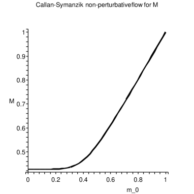
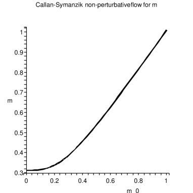
Figure 1: Non-perturbative flow for the dressed masses $M$ (scalar), $m$ (fermion) versus $m_{0}$. The dressed masses do not vanish when the bare mass $m_{0}$ goes to zero, due to dynamical mass generation.

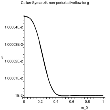
Figure 2: Non-perturbative flow for the dressed coupling $g$ versus $m_{0}$. Note that the one-loop correction to the coupling vanishes, explaining the small change in values for $g$.

3.5 IR stability

One can see from the one-loop expressions (3.4) that the limit $m_{0}\to 0$ leads to IR divergences. This is actually the case at any order of the loop expansion. Our numerical analysis shows that the resummation provided by the set of the coupled equations (42) restores the IR stability of the system, and that no divergence occurs in the dressed system, when $m_{0}\to 0$. Figs. 3 and 4 compare the one-loop and non-perturbative flows of $M$ and $m$ in the range of bare masses from $m_{0}/\Lambda=1$ down to $m_{0}=0$ (the region around $m_{0}=0$ is zoomed in, to highlight the difference). We clearly see with the fermion mass that the would-be IR divergence, in the limit where $m_{0}\to 0$, does not occur in the non-perturbative flow. This feature is a consequence of dynamical mass generation, which was already studied in the context of (2+1)-dimensional quantum electrodynamics ($QED_{3}$), following the present non-perturbative method [8].

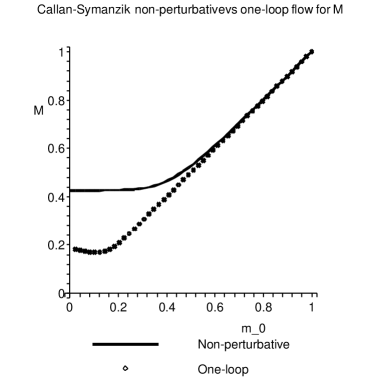
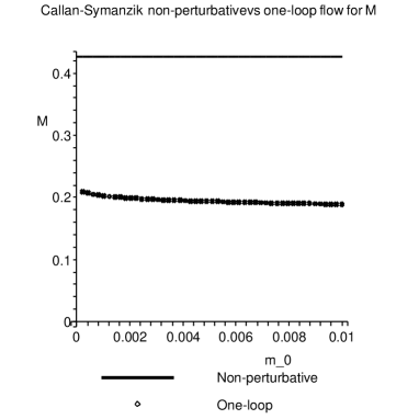
Figure 3: Comparison between the one-loop and the non-perturbative flows for the scalar dressed mass $M$ versus $m_{0}$ (the figure on the right is a zoom near $m_{0}=0$)

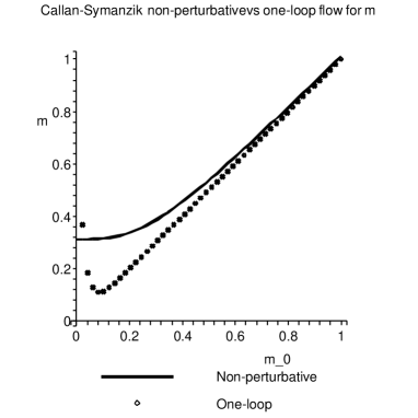
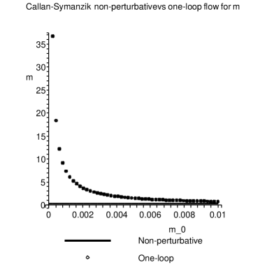
Figure 4: Comparison between the one-loop and the non-perturbative flows for the fermion dressed mass $m$ versus $m_{0}$ (the figure on the right is a zoom near $m_{0}=0$.

4 Comments on the gauged model

In this penultimate section, we would like to make some remarks concerning a possible extension of this Yukawa model to a gauged one, in which the fermions couple to an Abelian Gauge field. First, let us discuss a few features of the Lifshitz-type $QED$, which may be relevant for our purposes. Studies with anisotropic higher-order derivatives in $QED$ have already taken place in [9], but there, the Lorentz-violating terms are added to the usual Lorentz invariant $QED$. In the current article, we shall discuss a $QED$-type model, where only higher order derivatives are present in the model, as is the case of the Lifshitz-Yukawa model studied in previous sections.
We first note that the action for an Abelian gauge field in this framework, reads:

$$S_{g}=-\frac{1}{4}\int dtd^{3}{\bf x}\left\{2F_{0k}F^{0k}+G_{kl}G^{kl}\right\},$$ (44)

with $k,l=1,\cdots,D$ and

$$F_{0k}=\partial_{t}A_{k}-\partial_{k}A_{0}~{}~{}~{},~{}~{}~{}G_{kl}=-\Delta(\partial_{k}A_{l}-\partial_{l}A_{k}),$$ (45)

where $\Delta=\delta^{kl}\partial_{k}\partial_{l}$. The gauge fields have dimensionalities $[A_{0}]=2$ and $[A_{k}]=0$, and the action (44) is invariant under the gauge transformation $A_{\mu}\to A_{\mu}+\partial_{\mu}\theta$, where $[\theta]=-1$.
In order to find the gauge propagator, we first calculate the second functional derivatives of the action (44) with respect to the gauge fields,

$$\frac{\delta^{2}S_{g}}{\delta A_{0}\delta A_{0}} = -\Delta~{}\delta(t-t^{\prime})\delta^{(D)}({\bf x}-{\bf x}^{\prime})$$ (46)

$$\frac{\delta^{2}S_{g}}{\delta A_{0}\delta A_{k}} = -\partial_{t}\partial^{k}~{}\delta(t-t^{\prime})\delta^{(D)}({\bf x}-{\bf x}^{\prime})$$

$$\frac{\delta^{2}S_{g}}{\delta A_{k}\delta A_{l}} = \left[\eta^{kl}(\partial_{t}^{2}-\Delta^{3})-\Delta^{2}\partial^{k}\partial^{l}\right]\delta(t-t^{\prime})\delta^{(D)}({\bf x}-{\bf x}^{\prime})~{}.$$

In Fourier space, these read

$$\frac{\delta^{2}S_{g}}{\delta A_{0}\delta A_{0}} = {\bf p}^{2}~{}\delta(\omega-\omega^{\prime})\delta^{(D)}({\bf p}-{\bf p}^{\prime})$$ (47)

$$\frac{\delta^{2}S_{g}}{\delta A_{0}\delta A_{k}} = \omega p^{k}~{}\delta(\omega-\omega^{\prime})\delta^{(D)}({\bf p}-{\bf p}^{\prime})$$

$$\frac{\delta^{2}S_{g}}{\delta A_{k}\delta A_{l}} = \left[(({\bf p}^{2})^{3}-\omega^{2})\eta^{kl}+({\bf p}^{2})^{2}p^{k}p^{l}\right]~{}\delta(\omega-\omega^{\prime})\delta^{(D)}({\bf p}-{\bf p}^{\prime}).$$

Hence one can check that, for any $\mu=0,1,\cdots,D$,

$$\frac{\delta^{2}S_{g}}{\delta A_{\mu}\delta A_{\nu}}~{}p_{\nu}=\frac{\delta^{2}S_{g}}{\delta A_{\mu}\delta A_{0}}~{}\omega+\frac{\delta^{2}S_{g}}{\delta A_{\nu}\delta A_{k}}~{}p_{k}=0$$ (48)

which shows the absence of an inverse for the operator $\delta^{2}S_{g}$.

As usual, this is remedied by the addition of a gauge fixing term. In our Lifshitz case, this is naturally provided by the Coulomb gauge, which is equivalent to adding the term

$$-\frac{1}{2}\Delta^{2}\left(\partial^{k}A_{k}\right)^{2}$$ (49)

to the Lagrangian, so that the space components of the second derivatives (47) change to

$$\frac{\delta^{2}S_{g}}{\delta A_{k}\delta A_{l}}=(({\bf p}^{2})^{3}-\omega^{2})~{}\eta^{kl}~{}\delta(\omega-\omega^{\prime})\delta^{(D)}({\bf p}-{\bf p}^{\prime}).$$ (50)

Using the tensorial structure available in the $D$-dimensional space, we search for a gauge field propagator $D_{\mu\nu}(\omega,{\bf p})$ in the form

$$D_{00}=A,~{}~{}~{}~{}~{}~{}~{}~{}D_{0k}=Bp_{k},~{}~{}~{}~{}~{}~{}~{}~{}D_{kl}=C\eta_{kl}+Ep_{k}p_{l},$$ (51)

where $A,B,C,E$ are found from the definition

$$iD_{\mu\rho}~{}\frac{\delta^{2}S_{g}}{\delta A_{\rho}\delta A_{\nu}}=\delta^{\nu}_{\mu}~{}\delta(\omega-\omega^{\prime})\delta^{(D)}({\bf p}-{\bf p}^{\prime})~{}.$$ (52)

This leads to the following structures

$$D_{00} = \frac{-i}{{\bf p}^{2}}\left(1-\frac{\omega^{2}}{({\bf p}^{2})^{3}}\right)$$ (53)

$$D_{0k} = i\frac{\omega p_{k}}{({\bf p}^{2})^{4}}$$

$$D_{kl} = \frac{-i}{({\bf p}^{2})^{3}-\omega^{2}}\left(\eta_{kl}+\frac{\omega^{2}p_{k}p_{l}}{({\bf p}^{2})^{4}}\right).$$

In the Yukawa model discussed above, the scalar field is real and has no $U(1)$ charge. However, the (Dirac) fermion field can couple to the gauge field. This can be done in several ways, respecting gauge invariance. The minimal coupling can have one of the following forms

$$\overline{\psi}(i\partial_{t}-eA_{0})\gamma^{0}\psi-\overline{\psi}\left[\left(i\vec{\partial}-e{\bf A}\right)\cdot\vec{\gamma}\right]^{3}\psi$$

$$\overline{\psi}(i\partial_{t}-eA_{0})\gamma^{0}\psi-\overline{\psi}\left(i\vec{\partial}-e{\bf A}\right)^{2}\left(i\vec{\partial}-e{\bf A}\right)\cdot\vec{\gamma}~{}\psi$$ (54)

Since the gauge coupling is dimensionful ($[e]=1$), the quantum theory will exhibit fermion dynamical mass generation (the gauge boson remains massless because of gauge invariance). Therefore the model cannot describe massless fermions and, as in the Yukawa model, the fermion group velocity will be smaller than the speed of light.
The Lorentz-restoring kinetic terms arising from quantum fluctuations, for both the fermion and the gauge field, contain several contributions because of the new vertices appearing in the minimal couplings (4). Nevertheless, at one loop, the only contribution to the space components of the polarization tensor, which depends on the external momentum, is the same as the corresponding one in the Yukawa model, and is proportional to

$$\frac{g_{0}^{2}}{m_{0}^{2}}({\bf p}^{2}-p^{i}p^{j})~{}.$$ (55)

As we have already seen in the context of the Yukawa model above, this will lead to a speed of the gauge boson proportional to $g_{0}/m_{0}^{3}$. If we expect this gauge boson to represent a physical photon, then we need this speed to be of the order of the speed of light in vacuo (i.e. unity in our system of units). This implies that we have to be in a non-perturbative regime, where $g_{0}$ is of order of $m_{0}^{3}$, and, thus, the one-loop analysis is no longer valid. For this reason, a realistic study of the IR regime of this theory necessitates going beyond the one-loop approximation, which lies outside the scope of the current article, and thus is left for a future work.

5 Conclusions and Outlook

In this work we have examined the infrared limit of a Lifshitz-type Lorentz-violating Yukawa model, in (3+1)-dimensional Minkowski space time, where only higher order derivatives are present in the model. This differentiates the model, from existing ones in the literature, e.g. [9], where the Lorentz-violating terms co-exist, as small corrections, with the standard Lorentz-invariant ones. In our case, it is demonstrated that quantum corrections restore relativistic-like kinematics in the low energy-momentum regime (IR) of the model. In this way one can talk about a dynamically emergent Lorentz Invariance in the model, where each particle sees a different effective light cone. The group velocities of the fermions are found much smaller than those of the scalar field, although both velocities are much smaller compared to the speed of light in vacuo, consistent with the IR limit, where the analysis is performed.

Moreover, we have discussed a detailed mechanism for dynamical mass generation in the model in the same regime of low-energies. It is demonstrated that there is no massless limit in this model, in the sense that the quantum-fluctuations dressed masses never vanish, even in the limit where the bare masses go to zero. The model exhibits infrared stability, in the sense that the zero-bare-mass limit corresponds to infrared-divergence-free resummed quantum corrections. In our approach the resummation is provided by a differential Schwinger-Dyson type of approach, in which the relevant dressed parameters of the model appear in a set of coupled differential functional equations. We solved numerically these equations for the dressed mass and Yukawa coupling, and arrived at the aforementioned results on the IR stability and non-vanishing dynamically generated masses.

We also discussed briefly an extension of the model, which involves coupling of the fermions to an Abelian gauge field. The induced dispersion relations for the gauge field, which remains massless if we want to preserve the gauge invariance, are such that its velocity is also found much smaller than the speed of light in vacuo, thereby hampering any interpretation of such gauge fields as the physical photons.

In view of the above properties, a natural question arises as to what physical systems, if any, such classes of models might correspond to. In view of the emergent Lorentz symmetry, one might view our model as a toy model for explaining a rather microscopic origin of Lorentz symmetry, in the low-energy limit, in analogy with the case of condensed matter systems, with nodes in their Fermi surface, where linearization about them leads to low-energy relativistic excitations. Such a Lifshitz-type scenario, with emergent Lorentz symmetry, could survive the full inclusion of the Standard Model group, since the presence of several coupling constants would allow a fine tuning of parameters of the model, in such a way that the effective light cone seen by different species of particles could be made identical.

Another possible application of the (gauged) Yukawa model studied here, would be its association with the continuum limit of some Lattice models of potential relevance to some condensed matter systems in four space-time dimensions, in analogy with the case of planar high temperature superconductivity, where the gauge fields represent fractional statistics in (2+1)-dimensions. In such models, the gauge field is also different from the real photon, as in the gauged model of section 4. Thus, one may view the neutral scalar as a (spinless) phonon excitation, e.g. due to lattice ion vibrations, while the charged Dirac fermion could represent a spin mode coupled to an appropriate gauge potential, which, however, is not the physical photon. In condensed matter systems, the relativistic fermions may be associated with excitations near a node in the Fermi surface of the microscopic model [10]. From our analysis in section 4, one may assume that the massless gauge boson group velocity may represent the velocity of the node of the Fermi surface about which we linearized the continuum-model. In such a case, the physical significance of the gauge potential may be similar to that of a (3+1)-dimensional statistics-changing field for the fermion excitations, which could represent some kind of hole excitations, due to doping.

Acknowledgements J. A. would like to thank P. Pasipoularides and A. Tsapalis for useful comments. This work is partially supported by the Royal Society, UK, the European Union (N.E.M.), through the Marie Curie Research and Training Network UniverseNet (MRTN-2006-035863), and the STFC UK (D. Y.), through a Graduate Research Quota Studentship.

Appendix A: One loop effective theory

One-loop scalar self energy

For external momentum ${\bf k}$ and vanishing external frequency, the one-loop scalar self energy is, after a Wick rotation,

$$\Sigma_{s} = -ig_{0}^{2}~{}\mbox{tr}\int\frac{d\omega}{2\pi}\frac{d^{3}{\bf p}}{(2\pi)^{3}}\frac{i\omega\gamma^{0}-p^{2}({\bf p}\cdot\vec{\gamma})+m_{0}^{3}}{\omega^{2}+p^{6}+m_{0}^{6}}$$ (56)

$$~{}~{}~{}~{}~{}\times\frac{i\omega\gamma^{0}-({\bf p}+{\bf k})^{2}(({\bf p}+{\bf k})\cdot\vec{\gamma})+m_{0}^{3}}{\omega^{2}+({\bf p}+{\bf k})^{6}+m_{0}^{6}}.$$

The scalar mass correction is given by the zeroth order in ${\bf k}$, which is

$$\Sigma_{s}^{(0)} = 4ig_{0}^{2}\int\frac{d\omega}{2\pi}\frac{d^{3}{\bf p}}{(2\pi)^{3}}\frac{\omega^{2}+p^{6}-m_{0}^{6}}{(\omega^{2}+p^{6}+m_{0}^{6})^{2}}$$ (57)

$$= \frac{ig_{0}^{2}}{\pi^{2}}\int\frac{p^{8}dp}{(p^{6}+m_{0}^{6})^{3/2}}$$

$$= \frac{ig_{0}^{2}}{\pi^{2}}\left[\ln\left(\frac{\Lambda}{m_{0}}\right)+\frac{\ln 2-1}{3}\right]+{\cal O}(\Lambda^{-2}),$$

and we finally obtain for the scalar mass

$$M^{6}_{(1)}=m_{0}^{6}+\frac{g_{0}^{2}}{\pi^{2}}\left[\ln\left(\frac{\Lambda}{m_{0}}\right)+\frac{\ln 2-1}{3}\right]~{}.$$ (58)

The term quadratic in spatial derivatives is given by the quadratic-order term in the Taylor expansion of the self energy (56) in powers of ${\bf k}$:

$$\Sigma_{s}^{(2)} = 4ig_{0}^{2}\int\frac{d\omega}{2\pi}\frac{d^{3}{\bf p}}{(2\pi)^{3}}\Bigg{\{}\frac{p^{4}k^{2}+2p^{2}({\bf p}\cdot{\bf k})^{2}}{{\cal D}^{2}}-18p^{8}\frac{({\bf p}\cdot{\bf k})^{2}}{{\cal D}^{3}}$$

$$+\frac{\omega^{2}+p^{6}-m_{0}^{6}}{{\cal D}^{3}}\left(-3p^{4}k^{2}-12p^{2}({\bf p}\cdot{\bf k})^{2}+\frac{36p^{8}({\bf p}\cdot{\bf k})^{2}}{{\cal D}}\right)\Bigg{\}}$$

where ${\cal D}=\omega^{2}+p^{6}+m_{0}^{6}$. Using then the following identity, valid for any function $f$,

$$\int\frac{d^{3}{\bf p}}{(2\pi)^{3}}({\bf p}\cdot{\bf k})^{2}f(p^{2})=\frac{4\pi k^{2}}{3(2\pi)^{2}}\int dp~{}p^{4}f(p^{2}),$$ (60)

we obtain

$$\Sigma_{s}^{(2)} = \frac{ig_{0}^{2}k^{2}}{\pi^{3}}\int dp~{}p^{2}\int d\omega\left(-\frac{16p^{4}}{3{\cal D}^{2}}+\frac{6p^{10}+14m_{0}^{6}p^{4}}{{\cal D}^{3}}-\frac{24m^{6}p^{10}}{{\cal D}^{4}}\right)$$ (61)

$$= -\frac{ig_{0}^{2}k^{2}}{\pi^{2}m_{0}^{2}}\int_{0}^{\infty}\frac{dx~{}x^{6}}{(1+x^{6})^{3/2}}\left(\frac{8}{3}-\frac{3(3x^{6}+7)}{4(1+x^{6})}+\frac{15x^{6}}{2(1+x^{6})^{2}}\right).$$

The latter result has to be identified with $i\lambda_{\phi}^{(1)}k^{2}$, which leads to the expression (10) for $\lambda_{\phi}^{(1)}$, with a negative sign.

One-loop fermion self energy

The one-loop fermion self energy is, for external momentum ${\bf k}$ and vanishing external frequency, after a Wick rotation,

$$\Sigma_{f}=ig^{2}\int\frac{d^{3}{\bf p}}{(2\pi)^{3}}\frac{d\omega}{2\pi}\frac{\omega\gamma^{0}-p^{2}({\bf p}\cdot\vec{\gamma})+m_{0}^{3}}{{\cal D}}\frac{1}{\omega^{2}+({\bf p}-{\bf k})^{6}+m_{0}^{6}}.$$ (62)

The correction to the fermion mass is obtained from the zeroth-order term in ${\bf k}$:

$$\Sigma_{f}^{(0)} = \frac{ig_{0}^{2}}{(2\pi)^{4}}\int d^{3}{\bf p}d\omega\frac{m_{0}^{3}}{{\cal D}^{2}}$$ (63)

$$= \frac{ig_{0}^{2}m_{0}^{3}}{8\pi^{2}}\int\frac{p^{2}dp}{(p^{6}+m_{0}^{6})^{3/2}},$$

which yields

$$m^{3}=m_{0}^{3}+\frac{g_{0}^{2}}{24\pi^{2}m_{0}^{3}}.$$ (64)

The term linear in the spatial derivatives is given by the first-order term in the Taylor expansion in powers of ${\bf k}$:

$$\Sigma_{f}^{(1)} = -\frac{6g_{0}^{2}}{(2\pi)^{4}}\int d^{3}{\bf p}d\omega\frac{p^{6}({\bf p}\cdot\vec{\gamma})({\bf p}\cdot{\bf k})}{{\cal D}^{3}}$$ (65)

$$= -\frac{ig_{0}^{2}}{2\pi^{3}}({\bf k}\cdot\vec{\gamma})\int\frac{p^{10}dpd\omega}{{\cal D}^{3}}$$

$$= \frac{-3ig_{0}^{2}}{16\pi^{2}}({\bf k}\cdot\vec{\gamma})\int\frac{p^{10}~{}dp}{(p^{6}+m_{0}^{6})^{5/2}}.$$

This expression has to be identified with $-i\lambda_{\psi}^{(1)}({\bf k}\cdot\vec{\gamma})$, which leads to the expression

$$\lambda_{\psi}^{(1)}=\frac{3g_{0}^{2}}{16\pi^{2}}\int\frac{p^{10}~{}dp}{(p^{6}+m_{0}^{6})^{5/2}}.$$ (66)

One-loop vertex

We show here that the one-loop correction to the coupling vanishes. This correction is given by the following three-point graph, for vanishing incoming momentum:

$$g^{(1)}=g_{0}+ig_{0}^{3}~{}\mbox{tr}\int\frac{d\omega}{2\pi}\frac{d^{3}{\bf p}}{(2\pi)^{3}}\frac{\left(\omega\gamma^{0}-{\bf p}^{2}({\bf p}\cdot\gamma)+m_{0}^{3}\right)^{2}}{\left(\omega^{2}-p^{6}-m_{0}^{6}+i\varepsilon\right)^{3}},$$ (67)

and, after a Wick rotation,

$$g^{(1)} = g_{0}+\frac{g_{0}^{3}}{\pi^{3}}\int d\omega~{}p^{2}dp\frac{-\omega^{2}-p^{6}+m_{0}^{6}}{(\omega^{2}+p^{6}+m_{0}^{6})^{3}}$$

$$= g_{0}+\frac{g_{0}^{3}}{4\pi^{2}}\int p^{2}dp\left(\frac{3m_{0}^{6}}{(p^{6}+m_{0}^{6})^{5/2}}-\frac{2}{(p^{6}+m_{0}^{6})^{3/2}}\right)$$

$$= g_{0}+\frac{g_{0}^{3}}{12\pi^{2}m_{0}^{6}}\int_{0}^{\infty}dx\left(\frac{3}{(1+x^{2})^{5/2}}-\frac{2}{(1+x^{2})^{3/2}}\right)$$

The last integral vanishes, and $g^{(1)}=g_{0}$.

Appendix B: Evolution equations for the scalar potentials

Taking into account the gradient expansion (36) for the constant-field case $\phi_{cl}\rightarrow\phi_{0}$ and $\overline{\psi}_{cl}\psi_{cl}\rightarrow\xi_{0}$ leads to

$$\frac{\delta^{2}\Gamma}{\delta\phi_{p}\delta\phi_{q}} = \bigg{[}\omega^{2}-p^{6}-U^{\prime\prime}\xi_{0}-V^{\prime\prime}\bigg{]}\delta^{4}(p+q)\equiv\Gamma^{(2)}_{\phi\phi}\delta^{4}(p+q)$$

$$\frac{\delta^{2}\Gamma}{\delta\overline{\psi}_{p}\delta\psi_{q}} = \bigg{[}\gamma^{0}\omega-p^{2}({\bf p}\cdot\vec{\gamma})+U\bigg{]}\delta^{4}(p+q)\equiv\Gamma^{(2)}_{\overline{\psi}\psi}\delta^{4}(p+q)$$

$$\frac{\delta^{2}\Gamma}{\delta\psi\delta\overline{\psi}} = \bigg{[}\gamma^{0}\omega-p^{2}({\bf p}\cdot\vec{\gamma})-U\bigg{]}\delta^{4}(p+q)\equiv\Gamma^{(2)}_{\psi\overline{\psi}}\delta^{4}(p+q)$$

$$\frac{\delta^{2}\Gamma}{\delta\phi_{p}\delta\overline{\psi}_{q}} = -U^{\prime}\psi_{cl}\delta^{4}(p+q)\equiv\Gamma^{(2)}_{\overline{\psi}\phi}\delta^{4}(p+q)$$

$$\frac{\delta^{2}\Gamma}{\delta\phi_{p}\delta\psi_{q}} = U^{\prime}\overline{\psi}_{cl}\delta^{4}(p+q)\equiv\Gamma^{(2)}_{\psi_{p}\phi_{q}}\delta^{4}(p+q)$$ (68)

We have to calculate the inverse of the matrix

$$\Gamma^{(2)}=\left(\begin{array}[]{ccc}\Gamma^{(2)}_{\overline{\psi}\psi}&\Gamma^{(2)}_{\overline{\psi}\overline{\psi}}&\Gamma^{(2)}_{\overline{\psi}\phi}\\ \Gamma^{(2)}_{\psi\psi}&\Gamma^{(2)}_{\psi\overline{\psi}}&\Gamma^{(2)}_{\psi\phi}\\ \Gamma^{(2)}_{\phi\psi}&\Gamma^{(2)}_{\phi\overline{\psi}}&\Gamma^{(2)}_{\phi\phi}\\ \end{array}\right),$$ (69)

that we find by using the following expansion, valid for any two $3\times 3$ matrices $A,B$

$$(A+\xi_{0}B)^{-1}=A^{-1}-A^{-1}BA^{-1}\xi_{0}+{\cal O}(\xi_{0}^{2}).$$ (70)

In our case, this expansion gives for the elements of the inverse matrix $[\Gamma^{(2)}]^{-1}$,

$$[\Gamma^{(2)}]^{-1}_{\phi\phi}=\frac{1}{\omega^{2}-p^{6}-V^{\prime\prime}}$$ (71)

$$+\frac{\xi_{0}}{(\omega^{2}-p^{6}-V^{\prime\prime})^{2}}\times\left[U^{\prime\prime}-\frac{2[U^{\prime}]^{2}U}{(\gamma^{0}\omega-p^{2}({\bf p}\cdot\vec{\gamma}))^{2}-U^{2}}\right]+{\cal O}(\xi_{0}^{2}),$$

$$=I_{1}+\xi_{0}I_{2}+{\cal O}(\xi_{0}^{2}),$$

and

$$[\Gamma^{(2)}]^{-1}_{\overline{\psi}\psi}=\frac{1}{\gamma^{0}\omega-p^{2}({\bf p}\cdot\vec{\gamma})+U}$$ (72)

$$+\frac{-2\xi_{0}[U^{\prime}]^{2}U}{\bigg{[}\gamma^{0}\omega-p^{2}({\bf p}\cdot\vec{\gamma})+U\bigg{]}\bigg{[}\left(\gamma^{0}\omega-p^{2}({\bf p}\cdot\vec{\gamma})\right)^{2}-U^{2}\bigg{]}\bigg{[}\omega^{2}-p^{6}-V^{\prime\prime}\bigg{]}}$$

$$+\frac{-\xi_{0}[U^{\prime}]^{2}}{\bigg{[}(\gamma^{0}\omega-p^{2}({\bf p}\cdot\vec{\gamma}))^{2}-U^{2}\bigg{]}\bigg{[}\omega^{2}-p^{6}-V^{\prime\prime}\bigg{]}}+\mathcal{O}(\xi_{0}^{2})$$

$$=I_{3}+\xi_{0}I_{4}+{\cal O}(\xi_{0}^{2}),$$

After a Wick rotation, the integration over $(\omega,{\bf p})$ gives, for large values of $\Lambda$:

$$\mbox{Tr}\{I_{1}\} = \frac{-i{\cal V}}{12\pi^{2}}\ln\left(\frac{2\Lambda^{3}}{[V^{\prime\prime}]^{\frac{1}{2}}}\right)$$ (73)

$$\mbox{Tr}\{I_{2}\} = \frac{i{\cal V}}{24\pi^{2}}\frac{U^{\prime\prime}}{V^{\prime\prime}}+\frac{i[U^{\prime}]^{2}U}{6\pi^{2}}\left[-\ln\left(\frac{U}{[V^{\prime\prime}]^{\frac{1}{2}}}\right)\frac{1}{(V^{\prime\prime}-U^{2})^{2}}-\frac{1}{2(V^{\prime\prime}-U^{2})V^{\prime\prime}}\right]$$

$$\mbox{Tr}\{I_{3}\} = {\cal V}\frac{iU}{12\pi^{2}}\ln\left(\frac{2\Lambda^{3}}{U}\right)$$

$$\mbox{Tr}\{I_{4}\} = {\cal V}\frac{-i[U^{\prime}]^{2}U^{2}}{6\pi^{2}}\left[\ln\left(\frac{U}{[V^{\prime\prime}]^{\frac{1}{2}}}\right)\frac{1}{(V^{\prime\prime}-U^{2})^{2}}+\frac{1}{2(V^{\prime\prime}-U^{2})U^{2}}\right]$$

$$+ \frac{i{\cal V}}{12\pi^{2}}\frac{[U^{\prime}]^{2}}{(V^{\prime\prime}-U^{2})}\ln\left(\frac{U}{[V^{\prime\prime}]^{\frac{1}{2}}}\right),$$

where ${\cal V}$ is the space time volume. The reader should notice that this volume factor cancels out in eq.(35), since it appears on both sides of the equation.

References

• [1] M. Visser, Phys. Rev.  D 80 (2009) 025011 [arXiv:0902.0590 [hep-th]]; B. Chen and Q. G. Huang, Phys. Lett.  B 683 (2010) 108 [arXiv:0904.4565 [hep-th]]; S. R. Das and G. Murthy, Phys. Rev.  D 80 (2009) 065006 [arXiv:0906.3261 [hep-th]], arXiv:0909.3064 [hep-th]; W. Chao, arXiv:0911.4709 [hep-th]; R. Iengo and M. Serone, arXiv:1003.4430 [hep-th]; G. Koutsoumbas and P. Pasipoularides, arXiv:1006.3199 [hep-th]; J. M. Romero, J. A. Santiago, O. Gonzalez-Gaxiola and A. Zamora, arXiv:1006.0956 [hep-th]; K. Anagnostopoulos, K. Farakos, P. Pasipoularides and A. Tsapalis, arXiv:1007.0355 [hep-th].
• [2] A. Dhar, G. Mandal and S. R. Wadia, Phys. Rev.  D 80 (2009) 105018 [arXiv:0905.2928 [hep-th]]; A. Dhar, G. Mandal and P. Nag, Phys. Rev.  D 81 (2010) 085005 [arXiv:0911.5316 [hep-th]].
• [3] J. Alexandre, K. Farakos and A. Tsapalis, Phys. Rev.  D 81 (2010) 105029 [arXiv:1004.4201 [hep-th]].
• [4] J. Alexandre, K. Farakos, P. Pasipoularides and A. Tsapalis, Phys. Rev.  D 81 (2010) 045002 [arXiv:0909.3719 [hep-th]].
• [5] P. Horava, Phys. Rev.  D 79 (2009) 084008 [arXiv:0901.3775 [hep-th]].
• [6] R. Iengo, J. G. Russo and M. Serone, JHEP 0911 (2009) 020 [arXiv:0906.3477 [hep-th]].
• [7] J. Alexandre and J. Polonyi, Annals Phys.  288 (2001) 37 [arXiv:hep-th/0010128].
• [8] J. Alexandre, Annals Phys.  312 (2004) 273 [arXiv:hep-th/0310093].
• [9] D. Anselmi, Phys. Rev.  D 79 (2009) 025017 [arXiv:0808.3475 [hep-ph]]; Eur. Phys. J.  C 65 (2010) 523 [arXiv:0904.1849 [hep-ph]].
• [10] For a partial list of references see: G. Baskaran and P. W. Anderson, Phys. Rev.  B 37 (1988) 580; R. B. Laughlin, Science 242 (1988) 525. N. Dorey and N. E. Mavromatos, Phys. Lett.  B 250 (1990) 107; Nucl. Phys.  B 386 (1992) 614; G. W. Semenoff and N. Weiss, Phys. Lett.  B 250 (1990) 117; A. Kovner and B. Rosenstein, Phys. Rev.  B 42 (1990) 4748; J. Polchinski, arXiv:hep-th/9210046. K. Farakos and N. E. Mavromatos, Phys. Rev.  B 57 (1998) 3017 [arXiv:cond-mat/9611072]; L. Balents, M. P. A. Fisher and C. Nayak, arXiv:cond-mat/9803086. N. E. Mavromatos and S. Sarkar, Phys. Rev.  B 62 (1999) 3438 [arXiv:cond-mat/9912323]; J. Alexandre, N. E. Mavromatos and S. Sarkar, Int. J. Mod. Phys.  B 17 (2003) 2359 [arXiv:cond-mat/0303611]; N. E. Mavromatos and J. Papavassiliou, arXiv:cond-mat/0311421; I. F. Herbut, Phys. Rev. Lett.  94 (2005) 237001 [arXiv:cond-mat/0410557]; S. Sachdev, M. A. Metlitski, Y. Qi and C. Xu, Phys. Rev. B 80 (2009) 155129.