12 mm line survey of the dense molecular gas towards the W28 field TeV gamma-ray sources.

Abstract

We present 12 mm Mopra observations of dense molecular gas towards the W28 supernova remnant (SNR) field. The focus is on the dense molecular gas towards the TeV gamma-ray sources detected by the H.E.S.S. telescopes, which likely trace the cosmic-rays from W28 and possibly other sources in the region. Using the NH₃ inversion transitions we reveal several dense cores inside the molecular clouds, the majority of which coincide with high-mass star formation and Hii regions, including the energetic ultra-compact Hii region G5.89-0.39. A key exception to this is the cloud north east of W28, which is well-known to be disrupted as evidenced by clusters of 1720 MHz OH masers and broad CO line emission. Here we detect broad NH₃, up to the (9,9) transition, with linewidths up to 16 km s^-1. This broad NH₃ emission spatially matches well with the TeV source HESS J1801-233 and CO emission, and its velocity dispersion distribution suggests external disruption from the W28 SNR direction. Other lines are detected, such as HC₃N and HC₅N, H₂O masers, and many radio recombination lines, all of which are primarily found towards the southern high-mass star formation regions. These observations provide a new view onto the internal structures and dynamics of the dense molecular gas towards the W28 SNR field, and in tandem with future higher resolution TeV gamma-ray observations will offer the chance to probe the transport of cosmic-rays into molecular clouds.

1 Introduction

W28 (G6.4-0.1) is an old-age ($>10^{4}$ yr; Kaspi et al. 1993), mixed morphology supernova remnant (SNR) spanning 50${}^{\prime}\times 45^{\prime}$ with a distance estimated to be in the range 1.8 to 3.3 kpc (e.g. Goudis 1976; Lozinskaya 1981). The SNR exhibits non-thermal radio emission and thermal X-rays (Dubner et al., 2000; Rho & Borkowski, 2002), and more recently, gamma-ray sources at TeV (10¹² eV) (Aharonian et al., 2008b) and GeV (10⁹ eV) (Giuliani et al., 2010; Abdo et al., 2010) energies have been discovered by H.E.S.S., AGILE, and Fermi-LAT telescopes respectively, pointing to high energy particles in the region. ¹²CO (1–0), ¹²CO (2–1) and ¹²CO (3–2) surveys reveal massive molecular clouds to the north east (NE) and to the south (S) of the SNR (Arikawa et al., 1999; Reach et al., 2005; Torres et al., 2003; Aharonian et al., 2008b; Fukui et al., 2008). Most of the CO emission appears centred at a local standard of rest velocity V_LSR similar to that inferred for W28 V_LSR $\sim$7 km s^-1(or $\sim 2$ kpc) based on Hi studies (Velázquez et al., 2010). Torres et al. (2003) has argued that W28 has disrupted much of this CO gas, giving rise to its relatively broad velocity distribution. Notably, the NE region contains a rich concentration of 1720 MHz OH masers (Frail et al., 1994; Claussen et al., 1999) (with V_LSR in the range 5 to 15 km s^-1), and near-IR rovibrational H₂ emission (Reach et al., 2000; Neufeld et al., 2007; Marquez-Lugo et al., 2010), all indicating shocked gas which likely results from a SNR shock interaction with the NE molecular cloud. The southern region contains several Hii regions (G6.225-0.569, G6.1-0.6) including the ultra-compact (UC)-Hii region W28 A2 (G5.89-0.39), all indicating high-mass star formation. Additional SNRs have also been catalogued towards the W28 region, namely, G6.67-0.42 by Yusef-Zadeh et al. (2000), and G5.71-0.08 by Brogan et al. (2006). The $\sim$5 arcmin resolution H.E.S.S. TeV gamma-ray emission is resolved into four sources. HESS J1800-233 is situated towards the NE region where a SNR shock is known to interact with a molecular cloud, while a group of three TeV peaks are found towards the south coinciding with the Hii regions (HESS J1800-240A and B) and the SNR candiate G5.71-0.08 (HESS J1800-240C). Interestingly, a recently detected 1720 MHz OH maser (Hewitt & Yusef-Zadeh, 2009) towards G5.71-0.08, with V_LSR $=8$ km s^-1, may also suggest HESS J1800-240C is tracing a SNR/molecular cloud interaction. At lower angular resolution ($\sim$5 to 20 arcmin), two Fermi-LAT GeV sources, 1FGL J1800.5-2359c and 1FGL J1801.3-2322c (also detected by the AGILE detector) appear as counterparts to HESS J1800-233 and HESS J1800-240B respectively. Figure 1 compares the H.E.S.S. TeV emission with the 90 cm radio (VLA) image from Brogan et al. (2006), highlighting the prominent W28 SNR emission which peaks towards the NE interaction region, and G5.89-0.89 to the south.

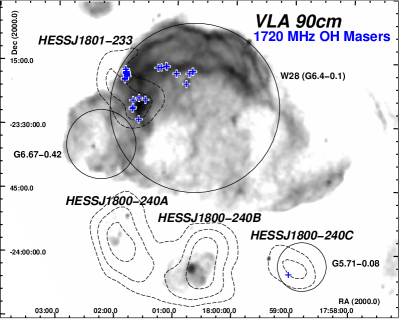
Figure 1: VLA 90 cm image (log scale up to 0.84 Jy/beam) from Brogan et al. (2006) of the W28 field with H.E.S.S. TeV emission (significance contours; black dashed). Boundaries of catalogued SNRs (black solid circles) and 1720 MHz OH masers from Claussen et al. (1999) and Hewitt & Yusef-Zadeh (2009) (blue $+$’s) are also indicated.

The TeV and GeV gamma-ray emission in the W28 region is spatially well-matched with the molecular clouds, and represents the best such match outside of the central molecular zone (CMZ) towards the Galactic Centre region (Aharonian at al., 2006). This, coupled with the old-age of W28, which would reduce any potential gamma-ray emission from accelerated electrons, suggests the gamma-ray emission results from collisions of cosmic-ray (CR) protons and nuclei with the molecular gas (Aharonian et al., 2008b; Fujita et al., 2009). W28 is a prominent member of a growing list of SNRs linked to TeV/GeV gamma-ray emission spatially matched with molecular clouds. This list includes HESS J1745-290/SNR G359.1-0.5 (Aharonian et al., 2004), HESS J1714-385/CTB 37A (Aharonian et al., 2008a), HESS J1923+141/SNR G49.2-0.7 (Feinstein et al., 2009), and IC 443 (Albert et al., 2008; Acciari et al., 2009). All of these SNRs exhibit 1720 MHz OH masers as for W28, and appear to be mature SNRs (age $>10^{4}$ yr) whereby any accelerated CRs would have begun to escape into the surrounding interstellar medium.

In the W28 field, the obvious source of CRs is the W28 SNR given its prominence in many wavebands, but the other SNRs in the region, all with unknown distances and ages, may contribute to CR acceleration. Moreover, the extensive star formation and Hii regions associated with the southern molecular clouds, in particular the energetic UC-Hii region G5.89-0.39 may also contribute CRs based on recent discussion of protostellar particle acceleration (Araudo et al., 2007). Some insight into where CRs are coming from can be obtained by looking at cloud density and emission line profiles in order to trace the presence and directionality of shocks.

Additionally, Gabici et al. (2007) showed that the energy and magnetic field dependent diffusion of CRs can lead to a hardening of the TeV gamma-ray emission spectrum as one looks inward towards dense molecular cloud cores (which typically span scale of a few arcminutes). Thus, spatial knowledge of molecular cloud density structures and cores towards TeV gamma-ray sources is a key step in probing the long sought-after diffusion properties of CRs.

Since the abundant ¹²CO molecular cloud tracer, with critical hydrogen density $\sim 10^{2-3}$ cm^-3, rapidly becomes optically thick towards molecular cloud clumps and cores, understanding of molecular cloud density profiles and internal dynamics can be impaired. Ideal tracers of dense gas such as NH₃ (ammonia), CS, and HC₃N are widely used due to their lower abundance (a factor $\sim 10^{-5}\times$CO) and higher critical densities $\sim 10^{4-5}$ cm^-3, which gives them a much lower optical thickness in dense gas. NH₃ is exceptionally useful since a single receiver at 23-25 GHz can detect a large number of NH₃ inversion transitions which are produced over a narrow bandwidth. Through satellite and hyperfine structure, these inversion transitions also allow the optical depth, and hence gas temperature and mass to be strongly constrained. Another desirable property of NH₃ is that the different inversion transitions cover a wide range of excitation conditions. NH₃ has therefore been detected in many astrophysical environments such as dense quiescent/cold gas and both warm to hot gas in low and high mass star formation regions. Indeed, virtually any region containing dense molecular material can be studied with an appropriate NH₃ transition (Ho & Townes, 1983). NH₃ is also known to exist in the coldest regions of molecular clouds depleting less rapidly from the gas phase compared to other common gas tracers, such as CO, which tends to freeze out onto dust grains (Bergin et al., 2006).

As the next step in probing the dense cores and dynamics of the W28 field molecular clouds, we have used the Mopra 22m single dish radio telescope in a 12 mm survey and single position-switched pointing covering the key inversion transitions of NH₃ and several other 12 mm lines tracing high-mass star formation including H₂O masers, HC₃N and CH₃OH.

2 Mopra Observations and Data Reduction

Observations were carried out on the Mopra radio telescope in May/June of 2008 and April of 2009 employing the Mopra spectrometer (MOPS) in zoom-mode.

Mopra is a 22 m single-dish radio telescope ($31^{\circ}16^{\prime}04^{\prime\prime}$S, $149^{\circ}05^{\prime}59^{\prime\prime}$E, 866m a.s.l.) located $\sim$450 km north west of Sydney, Australia. The 12 mm receiver operating in the frequency range of 16-27.5 GHz, coupled with the UNSW Mopra wide-bandwidth spectrometer (MOPS), allows an instantaneous 8 GHz bandwidth. This gives Mopra the ability to cover most of the 12 mm band and simultaneously observe many spectral lines. The zoom-mode of MOPS allows observations from up to 16 windows simultaneously, where each window is 137.5 MHz wide and contains 4096 channels in each of two polarisations. At 12 mm this gives MOPS an effective bandwidth of $\sim$ 1800 km s^-1  with resolution $\sim$ 0.41 km s^-1. Within this band the Mopra beam FWHM varies from 2.4^′ (19 GHz) to 1.7^′ (27 GHz) (Urquhart et al., 2010). Listed in Table 1 are some of the lines which are simultaneously within the bandpass in our configuration.

Table 1: Molecular lines and the corresponding rest frequencies which are detectable by the MOPS spectrometer in the configuration used. The final two columns indicate whether we detect the line in our maps or a deep pointing. Methanol (CH₃OH) masers are listed as type I or type II.

Molecular Line	Frequency	Detected	Detected
Name	(MHz)	Map	Deep Spectra
H69$\alpha$	19591.11	Yes	Yes
CH3OH(II)	19967.396	–	–
H86$\beta$	19978.17	–	Yes
H98$\gamma$	20036.32	–	Yes
NH3 (8,6)	20719.221	–	–
NH3 (9,7)	20735.452	–	–
C6H	20792.872	–	–
NH3 (7,5)	20804.83	–	–
NH3 (11,9)	21070.739	–	–
NH3 (4,1)	21134.311	–	–
H83$\beta$	22196.47	–	Yes
H2O Maser	22235.253	Yes	Yes
C2S	22344.030	–	–
H82$\beta$	23008.61	–	Yes
NH3 (2,1)	23098.819	–	–
CH3OH(II)	23121.024	–	–
H65$\alpha$	23404.28	Yes	Yes
CH3OH	23444.778	–	–
NH3 (1,1)	23694.4709	Yes	Yes
NH3 (2,2)	23722.6336	Yes	Yes
H81$\beta$	23860.87	–	Yes
NH3 (3,3)	23870.1296	Yes	Yes
CH3OH(I)	24928.715	–	–
CH3OH(I)	24933.468	–	–
CH3OH(I)	24934.382	–	–
CH3OH(I)	24959.079	–	–
CH3OH(I)	25018.123	–	–
NH3 (6,6)	25056.025	Yes	Yes
CH3OH(I)	25124.872	–	–
HC5N(10–9)	26626.533	Yes	Yes
H89$\gamma$	26630.71	–	Yes
H78$\beta$	26684.34	–	Yes
CH3OH(I)	26847.205	–	–
H62$\alpha$	26939.17	Yes	Yes
HC3N(3–2)	27294.078	Yes	Yes
CH3OH(I)	27472.501	–	–
NH3 (9,9)	27477.943	–	Yes

On-the-fly Mapping (OTF) observations were conducted in May of 2008, and consisted of four regions, which are referred as A (25^′ $\times$ $25^{\prime}$), B (20^′ $\times$ $20^{\prime}$) and C (15^′ $\times$ $15^{\prime}$) to cover the TeV emission peaks from HESS J1800-240 (Aharonian et al., 2008b) and map D (20^′ $\times$ $20^{\prime}$) to cover the TeV emission from HESS 1801-233 (Aharonian et al., 2008b). We mapped each region twice, scanning once in right ascension and once in declination in order to reduce noise levels and to eliminate artificial stripes that can be introduced when only one scanning direction is used. It also allows us to check for artefacts that may occur in one scan, but not the other. For reference, the mapped regions are indicated as dashed boxes in Figure 2.

The OTF mapping parameters we used are similar to those used in the the H₂O Southern Galactic Plane Survey (HOPS), a 12 mm study of the Galactic Plane (Walsh et al., 2008). Since HOPS also covered the W28 region, we have also included HOPS data in our mapping analysis, improving our exposure in the mapped areas B, C & D by a factor of two. Map A extended beyond the Galactic latitude limit of HOPS ($b=-0.5^{\circ}$) and so only partial overlap ($\sim$25%) exists.

Based on mapping results and prior knowledge of the regions under consideration, follow-up single pointing position-switched deep spectra were performed in June 2008 and in April of 2009, to provide high sensitivity to yield accurate measurement of the NH₃ (1,1) satellite lines which are necessary to determine the gas temperature and density. As we show shortly, several regions were found to exhibit NH₃ (1,1) and higher transitions with satellite lines apparent in the (1,1) spectra. Regions of bright NH₃ (1,1) emission from each map were targeted in these deep spectra. In total there were 10 regions which were selected for follow-up spectra which consisted of 1920 s (32 min) of ON source time.

Data were reduced using the ATNF packages  livedata,  gridzilla,  ASAP and Miriad. For mapping, livedata was used to perform a bandpass calibration for each row, using the preceding off scan as a reference and applied a 1^st order polynomial fit (i.e. linear) to the baseline. Gridzilla re-gridded and combined all data from all mapping scans onto a single data cube with pixels 15${}^{\prime\prime}\times 15^{\prime\prime}\times$0.43 km s^-1 ($x,y,z$). The mapping data are also weighted according to the relevant $T_{\rm SYS}$ , Gaussian-smoothed (2^′ FWHM and 5^′ cut-off radius) based on the Mopra beam FWHM $\theta_{\rm mb}=2^{\prime}$ appropriate for the NH₃ lines we detected, and pixel masked to remove noisy edge pixels. Analysis of position-switched deep pointings employed ASAP with time-averaging, weighting by the relevant $T_{\rm SYS}$ and baseline subtracted using a linear fit after masking of the 15 channels at each bandpass edge. In both mapping and position-switched data, the antenna temperature $T_{\rm A}^{*}$ (corrected for atmospheric attenuation and rearward loss) is converted to the main beam brightness temperature $T_{\rm mb}$ , such that $T_{\rm mb}$ = $T_{\rm A}^{*}$ $\eta_{\rm mb}$ where $\eta_{\rm mb}$ is the main beam efficiency. Based on the frequencies of the detected NH₃ lines ($\sim$24 GHz) we assume $\eta_{\rm mb}=0.6$ following Urquhart et al. (2010). This data reduction procedure yields an RMS error in $T_{\rm mb}$ of $T_{\rm rms}$ $\sim 0.05$ K per channel for mapping data with HOPS overlap and $T_{\rm rms}$ $\sim 0.08$ K per channel for mapping data without. As a result of their increased exposure, position-switched observations achieve a $T_{\rm rms}$ of $\sim 0.02$ K per channel.

3 Results Overview

Table 1 lists the lines detected in our mapping and position-switched deep spectra observations. In mapping data, the so called peak-pixel map for NH₃ (1,1) emission is shown in Figure 2 along with the locations of position-switched deep pointings.

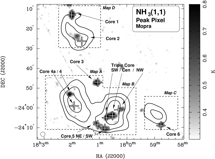
Figure 2: NH₃ (1,1) peak pixel emission [$T_{\rm mb}$ ] indicating the four mapped regions A,B,C,D in relation to the H.E.S.S. TeV emission (black contours 4, 5 and 6 $\sigma$ levels). HOPS data are also included. Black/white $+$ indicate the locations of the position-switched deep spectra summarised in Table 2.

Table 2: Coordinates of the Mopra 12 mm position-switched deep spectra observations and identification with the nearest TeV gamma-ray source. The position for Core 4 however, is taken from the mapping results since a position-switched observation was not taken.

Core Name	RA (J2000)	Dec. (J2000)
	hh:mm:ss	dd:mm:ss
Map D – HESS J1801-233
Core 1	18:01:59	-23:13:04
Core 2	18:01:37	-23:26:21
Map A – HESS J1800-240A
Core 3	18:01:03	-23:47:08
Core 4	18:02:04	-23:53:04
Core 4a	18:01:55	-23:59:05
Map B – HESS J1800-240B
Core 5 SW	18:00:48	-24:10:23
Core 5 NE	18:01:03	-24:08:38
Triple Core SE	18:00:45	-24:05:08
Triple Core Central	18:00:31	-24:04:09
Triple Core NW	18:00:18	-24:01:09
Map C – HESS J1800-240C
Core 6	17:58:46	-24:09:10

Peak-pixel maps highlight only the brightest pixel along the velocity axis ($z$ axis) and serve as a useful way to search for pointlike and moderately extended features.

Of the 29 molecular lines listed in Table 1 within the MOPS bandwidth, about half were detected. From the mapping observations we detected H₂O, NH₃ (1,1), NH₃ (2,2), NH₃ (3,3), NH₃ (6,6), HC₃N(3–2), HC₅N(10–9), H69$\alpha$, H65$\alpha$ and H62$\alpha$, with the criterion for detection being a 3 $T_{\rm rms}$ line peak signal. Since position-switched deep spectra observations were more sensitive than mapping, several additional lines were revealed as can be seen in Table 1. Maps of position-velocity (PV), integrated intensity, and spectra for all detected lines can be found in the online appendix.

3.1 NH₃

Presented in Figures 3, 4 and 5 are integrated intensity and position-velocity (PV) plots. The PV plots reveal the velocity-space structure of the NH₃ (1,1), (2,2) and (3,3) emission regions or cores in the W28 field. A Hanning smoothing in velocity (width $\sim$6 km s^-1) was applied to reduce random fluctuations, and then the Galactic latitude axis was flattened into a single layer. In this way we show the intrinsic velocity location and width of the gas without confusion. Based on the PV maps, it is clear that much of the NH₃ emission is found in the velocity range $\sim$-5 to $\sim$20 km s^-1  which is quite consistent with the molecular gas found in CO studies (Aharonian et al., 2008b; Fukui et al., 2008; Liszt et al., 2009) towards the W28 region. The four satellite lines of NH₃ (1,1) are clearly visible towards most of the cores as co-located peaks with 7 and 19 km s^-1  separation from the main line for the inner and outer satellite lines respectively. These satellite lines spread the (1,1) emission over a wider -20 to 50 km s^-1  range. The intensity maps also in Figures 3, 4 and 5 are integrated over V_LSR velocity ranges designed to encompass the bulk of the NH₃ emission, and show that it is found generally towards the TeV gamma-ray sources, and concentrated into clumps or cores. For simplicity we label the detected NH₃ features as Cores 1 to 6 and Triple Core with some of these containing sub-component clumps, for example, Triple Core Central, north west (NW) and south east (SE). Table 2 summarises the coordinates of the position-switched spectra towards each core, their relation to our dedicated mapping and overlapping TeV gamma-ray source.

In mapping data, most cores are seen in both NH₃ (1,1) and NH₃ (2,2) emission, whereas NH₃ (3,3) emission has been detected towards the Core 2, Core 5 SW and the Triple Core regions. In position-switch spectra, NH₃ (6,6) is detected towards Core 2 and Triple Core Central, while a weak detection of (9,9) is seen towards Core 2 (see online Figures for spectral plots). Such transitions are evidence of high gas temperature and potential disruption. Core 2 is exceptional in that it represents the well-known NE W28 SNR shock and molecular cloud interaction region as traced by broad CO emission and 1720 MHz OH masers towards HESS J1801-233. A prominent feature here is the broadness and relative intensities of NH₃ (3,3) and (6,6) compared to the (2,2) and (1,1) transitions. The Triple Core and Core 5 comprise several resolved clumps and are linked to the energetic Hii region G5.89-0.39 at the centre of HESS J1800-240B. Many of the other lines we detect in maps are found towards the Triple Core and Core 5, namely, bright and extended H₂O masers, radio recombination lines (RRL), and the cyanopolyynes HC₃N and HC₅N. Cores 4 and 4a appear to trace additional Hii regions towards HESS J1800-240A. Core 1 is possibly a star formation site just north of HESS J1801-233 and the NE SNR/molecular cloud interaction region. Cores 3 and 6 appear to have quite different velocities at $\sim$-25 km s^-1  to the other cores and are likely not connected with the molecular gas physically associated with the W28 region.

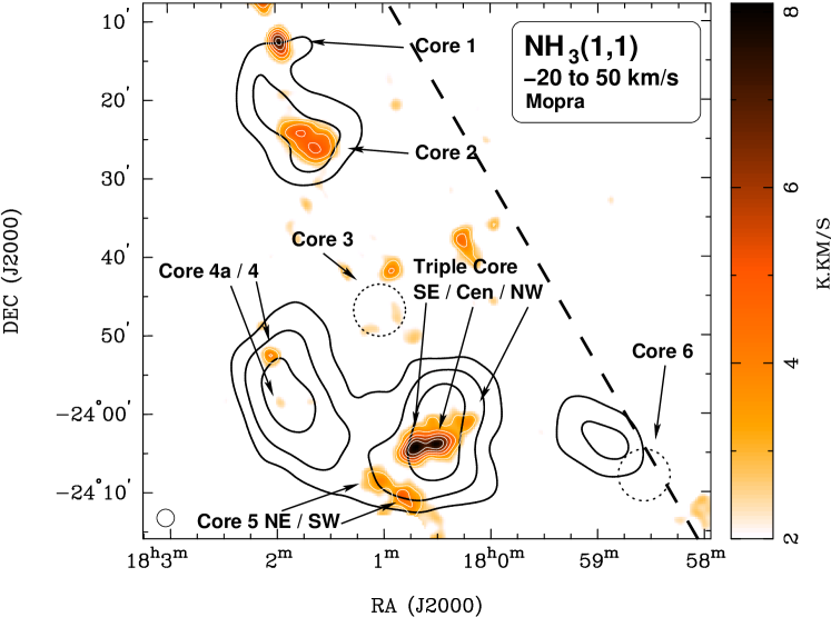
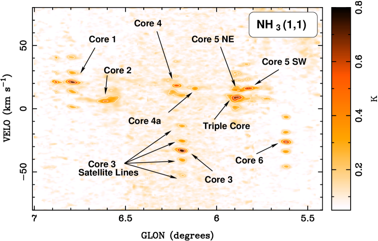
Figure 3: Top: Integrated intensity [$T_{\rm mb}$ ] map of Mopra NH₃ (1,1) emission integrated from -20 to 50 km s^-1  to encompass the various (1,1) cores towards the TeV emission (white contours are 3, 4, 5, 6, 7 K km s^-1). Identified cores are labeled as described in the text. Dashed line indicates the Galactic Plane, dashed circles indicate the location of Cores 3 and 6 which have centre velocities outside the integration range. The Mopra beam (2^′ FWHM) is indicated in the bottom left corner. Bottom: Position-Velocity (PV) map of the peak pixel NH₃ (1,1) emission (white contours 0.2, 0.4, and 0.6 K) indicating its velocity location and spread. For most cores the NH₃ (1,1) satellite peaks (e.g. labeled for Core 3) may be seen as four peaks surrounding the central one along the velocity axis.

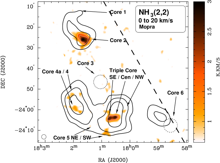
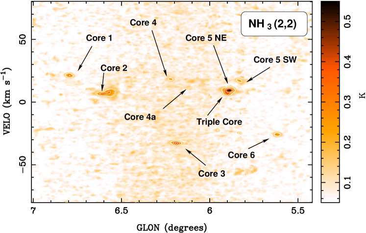
Figure 4: As for Figure 3 but showing NH₃ (2,2) integrated over 0 to 20 km s^-1  (white contours are 1.5, 2, 3 K km s^-1) and PV plot (white contours 0.18, 0.2, 0.3, and 0.4 K).

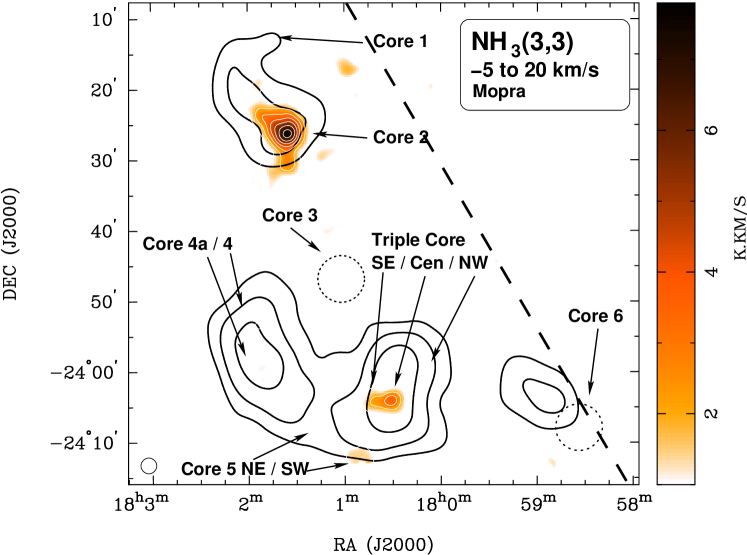
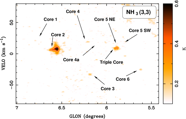
Figure 5: As for Figure 3 but showing NH₃ (3,3) integrated over -5 to 20 km s^-1  (white contours are 1, 2, 3, 4, 5, 6, 7 K km s^-1) and PV plot (white contours 0.2, 0.4, and 0.6 K).

3.2 Other 12 mm Line Detections: H₂O Masers, Radio Recombination Lines and Cyanopolyynes.

A number of other 12 mm lines are detected with mapping data over a velocity range consistent with the W28 clouds and our NH₃ detections. These are H₂O masers, the radio recombination lines (RRLs) H62$\alpha$, H65$\alpha$ and H69$\alpha$, and the cyanopolyyne lines HC₃N(3–2) and HC₅N(10–9). Maps integrated over the velocity range 5 to 20 km s^-1, covering the bulk of the detected emission and spectra for all of these detections can be found in the online Figures. The most prominent detection of H₂O masers, RRLs and cyanopolyynes is found towards the Triple Core region, reflecting the strong Hii and star formation activity there. Since the focus of this paper is the dense gas traced by NH₃, we only present the measured line parameters for the RRLs, cyanopolyynes and H₂O masers in our online appendix.

In the Triple Core, H₂O masers are detected in both the SE and Central regions. The SE emission contains large velocity structure, spread over 100 km s^-1. An additional H₂O maser is also seen towards Core 1. According to recent work with 12.2 GHz methanol masers (Breen et al., 2009) an evolutionary sequence for masers associated with high mass star formation regions has been suggested. This evolutionary sequence suggests that the presence of H₂O masers occurs between $\sim$1.5 to $4.5\times 10^{4}$ yr after high-mass star formation, encompassing the onset of an initial or hypercompact (HC) Hii region forming $\sim$ 2$\times 10^{4}$ yr after the high-mass star formation.

The radio recombination lines trace ionised gas which often exhibit very broad line widths as a result of likely pressure broadening and turbulence associated with ionised gas. The lines we see are no exception to this with several reaching line widths $>40$ km s^-1extending to $>100$ km s^-1  in the Triple Core Central and SE regions. Interestingly, the RRL emission appears to be extended and thus may allow probing of the extent to which ionisation is occuring within the southern, central molecular cloud. As indicated in Table 1 and the online appendix we detect 10 RRL transitions in total although only the strongest three transitions (H62$\alpha$, H65$\alpha$, H69$\alpha$) are detected in the mapping data.

The strongest cyanopolyyne HC₃N and HC₅N emission is found centred on Triple Core Central in mapping data but position-switched spectra reveal these molecules towards most of the other star formation cores (Core 1, 3, 4a, and 6) with a possible weak detection towards Core 2. These are long carbon chain molecules which tend to trace the earlier stages of core evolution while NH₃ tends to become more abundant at later stages (Suzuki et al., 1992). However recent work has indicated that HC_nN($n>3$) can be produced under hot core conditions for short periods of time. HC₃N is produced in large quantities at early times while HC₅N is created and destroyed within several hundred years, making it a potential chemical clock (Chapmann et al., 2009).

3.3 CO and Infrared Comparison

Our 12 mm line survey adds to the extensive list of molecular cloud observations devoted to the W28 SNR field. The Nanten telescope (Mizuno & Fukui, 2004) has mapped W28 in the ¹²CO (1–0) (Aharonian et al., 2008b) and (2–1) (Fukui et al., 2008) transitions, following on from earlier ¹²CO (1–0) (e.g. Arikawa et al. 1999; Dame et al. 2001; Reach et al. 2005; Liszt et al. 2009) and ¹³CO (1–0) studies (Kim & Koo, 2003). More recent large-scale surveys of ¹²CO (2–1) and small scale mapping of the Triple Core region (G5.89-3.89A and B) in ¹²CO (4-3) and ¹²CO (7-6) have been carried out by Nanten2 (Fukui et al., 2008). Our Mopra mapping was indeed guided by the Nanten CO results, which provide the most sensitive large-scale look at the molecular gas in the region. Figure 6 compares the Nanten2 ¹²CO (2–1) image with the NH₃ (1,1) and (3,3) emission from our Mopra observations, Nobeyama ¹²CO (1–0) and JCMT ¹²CO (3–2) observations by Arikawa et al. (1999) as well as the TeV gamma-ray emission with H.E.S.S. The ¹²CO (2–1) emission spatially matches well the brightest three TeV gamma-ray peaks as highlighted previously for the ¹²CO (1–0) emission by Aharonian et al. (2008b). This match is quite striking towards the Core 2/HESS J1801-233 region where broad ¹²CO (3–2) or shocked/disrupted gas tends to lie inward in the direction of W28 compared to the more quiescent and relatively narrower ¹²CO (1–0). Here, the NH₃ (3,3) emission reveals for the first time the dense and disrupted core of the shock-compressed NE molecular cloud. Towards the Triple Core region the Nanten2 ¹²CO (2–1) emission is resolved into two peaks assocated with the Hii regions G5.89-3.89A and B respectively. Core 5 NW and SW are also traced by ¹²CO (2–1) enhancements, which are also clearly seen in ¹³CO (1–0) (Kim & Koo, 2003). Our Mopra NH₃ emission also appears to resolve peaks associated with G5.89-3.89A and B, and Cores 5 NE and SW.

Figure 6: Left: Nanten ¹²CO (2–1) image [K km s^-1] (Fukui et al., 2008) in log scale, with contours of Mopra NH₃ (1,1) (white) and H.E.S.S. TeV gamma-ray significance (black-dashed). 1720 MHz OH masers from Claussen et al. (1999); Hewitt & Yusef-Zadeh (2009) are also indicated (blue/white $+$). Above: Core 2 zoom in linear scale with contours of ¹²CO (1–0) (magenta-dashed) and ¹²CO (3–2) (blue) from Arikawa et al. (1999). SNR diameters for W28 and other SNRs (Yusef-Zadeh et al., 2000; Brogan et al., 2006) are indicated in both panels.

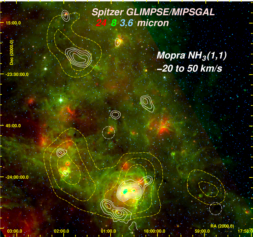
Figure 7: Spitzer GLIMPSE/MIPSGAL three colour (RGB=24/8/3.6 $\mu$m; MJy/sr in log scale) image with contours from Mopra NH₃ (1,1) emission (linear white contours $>$ 1.5 K) and H.E.S.S. TeV gamma-ray significance (yellow dashed).

Figure 7 presents the infrared (IR) Spitzer GLIMPSE and MIPSGAL three-colour (RGB=24/8/3.6 $\mu$m) image of the W28 region with Mopra NH₃ (1,1) and H.E.S.S. TeV gamma-ray contours. These IR bands are tracers of polycyclic aromatic hydrocarbons (PAHs) and dust emission, revealing the complexity of the W28 region in hosting several star formation and Hii regions in quite likely several different evolutionary stages. Table 3 summarises the likely counterparts identifed with our detected cores.

Further discussion of the individual cores and comparison of previous molecular line studies toward them can be found later in §5.

Table 3: Likely counterparts to the various cores detected. Counterparts have been searched for within a 2^′ radius using the SIMBAD^† astronomical database. Where a star is listed the spectral type is also given.

Core Name	Counterpart Name
Core 1	IRAS 17589-23121
Core 2	W28 SNR/Mol. cloud interaction
Core 3	HD 313632 (B8 IV)
Core 4	Hii 6.225-0.5692
Core 4a	Hii G6.1-0.63 / IRAS 17588-2358
Core 5 SW	IRAS 17578-2409
Core 5 NE	HD 164194 (B3II/III C)
	IRAS 17578-2409a
Triple Core SE	Hii G5.89-0.39A4 / W28-A2
Triple Core Central	Hii G5.89-0.39B4
Triple Core NW	V5561 Sgr (M) / IRC-204115
Core 6	IRAS 17555-2408b
1. Bronfman et al. (1996)
2. Lockman (1989)
3. Kuchar & Clark (1997)
4. see Kim & Koo (2001) and references therein.
5. Johnston et al. (1973).
$\dagger$ http://simbad.u-strasbg.fr/simbad/.
$a$. 2.8′ distant.
$b$. 2.3′ distant.

4 Analysis of NH₃ Emission

We describe here procedures used to estimate the gas parameters such as optical depth, temperature, mass, density, and related dynamical information towards the NH₃ cores. Tables4 (with statistical errors in the online appendix) and 5 summarise these results utilising the NH₃ (1,1) and (2,2) spectra for an analysis assuming various core sizes, and additional results treating Core 2, Triple Core and Core 5 as extended clouds well beyond the size of the 2^′ FWHM beam. We also apply a detailed radiative transfer model to Core 2, given its apparent high gas temperature and non-thermal energy.

4.1 Line Widths

The FWHM of the NH₃ main line, $\Delta\,v_{1/2}$, is a useful measure of the total energy associated with the core or clump. Broader lines will result from regions with higher temperatures or some additional dynamics. The purely Maxwell-Boltzmann thermal line width FWHM $\Delta\,v_{\rm th}$ expected from a gas at temperature $T$ is given by

$$\Delta v_{\rm th}\sim\sqrt{\frac{8~{}{\rm ln}(2)~{}k~{}T}{m_{\tiny{\textrm{NH}}_{3}}}}\hskip 8.53581pt\textrm{[\mbox{km\,s${}^{-1}$}]}$$ (1)

where $k$ is Boltzmann’s constant and $m_{\tiny{{\rm NH}}_{3}}$ is the mass of the NH₃ molecule. For example, a thermal line width of $\sim$0.16 km s^-1  is obtained for a temperature of 10 K, as might be expected in typically cold dense NH₃ cores (Ho & Townes, 1983). The line FWHM, $\Delta\,v_{1/2}$, of each core was estimated from a Gaussian fit to the central or main peak of the emission with additional Gaussians to fit each of the four satellite lines, which are generally resolved in the (1,1) transition. This five-Gaussian fit function can be seen applied to the Core 1 and Core 2 spectra in Figure 8. The results in Table 4 show that $\Delta\,v_{1/2}$ for all cores is considerably wider than that expected from purely thermal broadening, suggesting additional non-thermal or kinetic energy which dominates over broadening from the instrumental response, which is considered negligible.

4.2 Gas Parameters

The (1,1) satellite lines were clearly resolved in all cores except in Core 2 which is instrinsically very broad, leading to blending of the main and satellite lines (see Figure 8). Using the relative brightness temperatures of the main and satellite peaks, the optical depth can be derived for each ($J,K$) inversion transition by numerically solving Equation 2 of Barrett et al. (1977). A weighted average $\bar{\tau}(J,K,m)$ (with weight given as 1/peak-error according to the Gaussian fit) of the four satellite-derived optical depths is then calculated, and the total optical depth $\tau_{\rm J,K}^{\rm tot}$ of the transition is estimated by accounting for the fraction of intensity in the main line (where $f$(1,1)=0.502, and $f$(2,2)=0.796). Without needing to resolve the (2,2) satellite lines, the main line optical depth of the (1,1) transition can be used to infer the main line optical depth of the (2,2) transition using the method of Ungerechts et al. (1986). As for the (1,1) transition, a weighted average may be used to derive the total (2,2) optical depth $\tau_{\rm 2,2}^{\rm tot}$. The line FWHM is of critical consideration when determining the temperature of the gas, as a key assumption in this step is that both the (1,1) and (2,2) emission probe the same volume of gas. The similarity of FWHM for the (1,1) and (2,2) transitions in Table 4 does however suggest that both transitions originate from the same general volume of gas, allowing the rotational temperature to be calculated using the method of Ungerechts et al. (1986). Generally the rotational temperature is an underestimate of the kinetic temperature (Ho & Townes, 1983), however, the analytical expression of Tafalla et al. (2004, pg. 211) has been used to estimate $T_{\rm k}$ from $T_{\rm rot}$ . This is believed to be accurate to within 5% of the real value of $T_{\rm k}$ for temperatures in the 5-20 K range. Importantly, this method for obtaining temperatures is only considered valid for $T_{\rm k}$ up to $\sim$40 K. To obtain the column density for the NH₃ emission, we use the (1,1) transition and follow Equation 9 of Goldsmith & Langer (1999). Since the (1,1) represents only a fraction of the NH₃ gas, the total NH₃ column density $N_{\textrm{\tiny{NH}}_{3}}$ can be obtained from the (1,1) column density and the partition function $Q(T)$. In this work we assume contributions up to the $5^{\rm th}$ term in the series expansion.

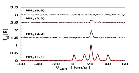
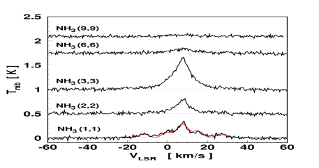
Figure 8: NH₃ (n,n) position-switched spectra for Core 1 (Left) and Core 2 (Right). Gaussian fits to the (1,1) and (2,2) spectra used to estimate gas parameters (see Table 4). The (1,1) fits are shown as red solid lines and the (n,n) spectra for n$\geq$2 are offset by a constant value for clarity.

To determine the total mass $M$ and molecular hydrogen number density $n_{\rm H_{2}}$ (hereafter referred as just density) of the various cores we need to assume the core intrinsic radius $R$ and the abundance ratio $\chi_{\textrm{\tiny{NH}}_{3}}$ of NH₃ to H₂. We note that the abundance ratio is known to depend on the gas temperature $T$. Ratios quoted in literature extend from $\sim$10^-7, few $\times 10^{-8}$ (Walmsley & Schilke, 1983; Ott et al., 2005), down to $\sim 10^{-10}$ Ott et al. (2010) in the Large Magellanic Cloud. For typical infrared dark clouds (IRDCs) with $T<20$ K an average value of $\sim 4\times 10^{-8}$ is found (Pillai et al., 2006). However with the exception of Core 2 and Core 6, all NH₃ cores in the W28 field are identified with star formation IR sources as indicated in Figure 7 and Table 3. In hot cores, with ($T>100$ K), abundance ratios of 10^-6 or even as high as 10^-5 have been suggested (Walmsley & Schilke 1983, 1992 and references therein). We adopt the value

$${\large\chi}_{\textrm{\tiny{NH}}_{3}}=N_{\textrm{\tiny{NH}}_{3}}\,/\,N_{\textrm{\tiny{H}}_{2}}=2\times 10^{-8}$$ (2)

following Stahler & Palla (2005, Table 5.1) as the temperatures of our detected cores are only slightly higher than those typical of IRDCs. The total hydrogen mass of the core is then estimated by factoring in the projected area of the emitting region:

$$M=fK\,2m_{\rm H}\,\pi R_{\rm cm}^{2}\,N_{\textrm{\tiny{NH}}_{3}}/({\large\chi}_{\textrm{\tiny{NH}}_{3}}\,{\rm M_{\odot}})\hskip 8.53581pt[{\rm M_{\odot}}]$$ (3)

for the core intrinsic radius expressed in cm units $R_{\rm cm}$ and $m_{\rm H}$ the hydrogen mass (kg). Following Urquhart et al. (2010) we apply the beam dilution factor $f$, given by $1/f=\ln 2\,(2R/\theta_{\rm mb})^{2}$, and beam coupling coefficient $K=x^{2}/[1-\exp(-x^{2})]$ for $x=\sqrt{1/f}$ in order to account for various source radii. Therefore the product $fK=1/[1-\exp(-1/f)]$ with $fK\rightarrow 1.0$ for increasing $R$.

The H₂ molecular number density $n_{\rm H_{2}}$ follows by accounting for the emitting volume of emission, assumed to be a sphere with radius $R_{\rm cm}$ in cm.

$$n_{H_{2}}=M\,{\rm M_{\odot}}/(2m_{\rm H}\,4/3\pi R_{\rm cm}^{3})\hskip 8.53581pt[\rm{cm}^{-3}]$$ (4)

Except for Core 2 and possibly the Triple Core and Core 5 complexes, the NH₃ emission appears to be point-like and thus has an intrinsic diameter upper limit approaching the 2^′ Mopra beam FWHM, or $R_{\rm mb}=0.5\theta_{\rm mb}=0.6$ pc radius assuming a 2 kpc distance (consistent with the W28 SNR). Although $R=0.1$ pc is typically noted as the intrinsic radius for cold dense cores (Ho & Townes, 1983), we assume a source radius of 0.2 pc as a default. The estimates for mass and density assuming a point-like source radius of $R=0.2$ pc are listed in Table 5. In order to allow for varying core radii, we also include scaling factors for the mass and density resulting from the source radius $R$ dependence in $fK$, source projected area, and volume.

In considering Core 2, Triple Core and Core 5 as extended regions, we calculate gas parameters from their NH₃ (1,1) and (2,2) spectra averaged over elliptical regions and for pixels $T_{\rm mb}$ $\geq 0.18$ K. The extended mass is estimated as in Eq. 3 using the column density averaged over the extended region of radius $R_{\rm cm}$ in cm, but with an extra term $\eta_{\rm mb}/\eta_{\rm xb}=0.86$ to account for the extended Mopra beam efficiency $\eta_{\rm xb}=0.7$ appropriate for the NH₃ lines (Urquhart et al., 2010). Density then follows from Eq. 4 as before. Results, including dimensions of the elliptical regions are given in Tables 4 and 5. Additionally for Core 2, we use the NH₃ (1,1) to (6,6) spectra (position-switched and mapping) in more detailed radiative transfer modeling discussed in $\S$4.4 to estimate gas parameters.

Under the assumption that the cores are in gravitational equilibrium with their thermal energy, their pure molecular hydrogen virial masses $M_{\rm vir}$ may also be estimated:

$$M_{\rm vir}=k\,R\,(\Delta v_{1/2})^{2}\hskip 8.53581pt[\rm{M}_{\odot}]$$ (5)

for the source radius $R$ (pc) as before and $\Delta v_{1/2}$ the line FWHM ( km s^-1). The factor $k$ depends on the assumed mass density profile of the core $\rho(r)$ with radius $r$. For a Gaussian density profile Protheroe et al. (2008) calculates $k=444$, in contrast to other situations such as a constant density ($k=210$) and $\rho\propto r^{-2}$ ($k=126$) (MacLaren, 1988). Although a Gaussian profile is quite likely, we quote here in Table 5 the virial masses bounded by the Gaussian and $r^{-2}$ density profiles with a source radius $R$=0.2 pc. Additionally, an overestimate of the true core line FWHM can result for optically thick lines. Given the similarity of the NH₃ (1,1) and (2,2) linewidths, and that the (2,2) optical depth is generally less than unity (see Table 4), we use the (2,2) FWHM in the virial mass calculation. The exception is for Core 2 analysis in which case we use the (3,3) linewidth. Overall, the virial masses we derive here could be considered upper limits, especially in the case of a Gaussian density profile. Nevertheless, the virial mass serves as an important guide in understanding the stability of the cores.

By far the dominant systematic error in our mass and density estimates arises from the uncertainty in the NH₃ abundance ratio ${\large\chi}_{\textrm{\tiny{NH}}_{3}}$. Given the range of ratios quoted in literature for cores of similar temperature to ours, we quote systematic errors of a factor 2 to 5 for ${\large\chi}_{\textrm{\tiny{NH}}_{3}}$, which feed directly into mass and density. Given that most of the core masses we derive are in agreement with their virial mass range (Table 5), our choice of ${\large\chi}_{\textrm{\tiny{NH}}_{3}}=2\times 10^{-8}$ appears reasonable.

Table 4: NH₃ gas parameters derived from NH₃ (1,1) and (2,2) spectra. Results for point-like analysis are taken from a single position (either from position-switched data or from mapping data in the case of Core 4). Extended source parameters are taken from spectra averaged over an elliptical region given below and for pixels satisfying a $T_{\rm mb}$ $\geq 0.18$ K masking level in mapping observations. Columns from left to right are core name, integrated intensity for (1,1), (2,2) and (3,3), rotational temperature $T_{\rm rot}$ , kinetic temperature $T_{\rm k}$ , NH₃ (1,1,m) main line velocity V_LSR , main line FWHM $\Delta\,v_{1/2}$ for (1,1), (2,2), and (3,3), total column density $N_{\textrm{\tiny{NH}}_{3}}$, and total optical depth $\tau_{\rm 1,1}^{\rm tot}$ and $\tau_{\rm 2,2}^{\rm tot}$ for (1,1) and (2,2) respectively. Statistical errors are given in the online appendix.

Core/Region Name	$\int\,\mbox{$T_{\rm mb}$\,}\,dv$	$T_{\rm rot}$	$T_{\rm k}$ †	VLSR	$\Delta\,v_{1/2}$	$N_{\textrm{\tiny{NH}}_{3}}$	$\tau$
	[K km s-1]	[K]	[K]	[km s-1]	[km s-1]	[1013 cm-2]
	(1,1)/(2,2)/(3,3)			(1,1,m)	(1,1,m)/(2,2,m)/(3,3,m)		$\tau_{\rm 1,1}^{\rm tot}$/$\tau_{\rm 2,2}^{\rm tot}$
—– Point Source Analysis —–
Core 1	7.6/1.6/0.5	16.0	18.4	+21	2.8/2.9/3.3	36.4	2.7/0.5
Core 2	4.7/2.5/7.4/1.3/0.3‡	29.9	46.4	+7	6.3/9.7/12.8/15.9/13.8‡	17.8	2.2/1.3
Core 3	8.6/2.5/1.4	17.4	20.4	$-$33	3.2/3.3/4.7	46.8	3.2/0.7
Core 4	3.8/0.6/—	17.9	20.7	+18	1.9/1.8/—	14.2	2.1/0.5
Core 4a	2.1/0.7/0.4	20.0	24.9	+16	2.9/3.0/3.4	5.5	1.2/0.4
Core 5 SW	6.0/1.1/0.5	15.6	17.8	+16	2.3/2.3/3.1	25.6	2.3/0.4
Core 5 NE	3.4/0.4/0.2	11.6	12.4	+15	1.8/2.0/4.9	24.8	3.0/0.2
Triple Core SE	7.8/3.1/1.7	20.6	25.8	+9	3.4/3.6/4.5	35.0	2.8/0.9
Triple Core Cen.	8.4/4.2/3.5	24.2	32.6	+9	3.9/4.5/5.8	23.4	1.5/0.6
Triple Core NW	2.6/0.6/0.4	18.6	22.4	+10	2.4/2.1/2.5	9.7	2.2/0.5
Core 6	7.9/1.5/0.9	14.4	16.1	$-$26	3.0/2.9/3.8	67.0	4.6/0.6
—– Extended Source Analysis —–
Core 21	3.4/1.5/3.5	25.2	34.8	+7	6.2/8.6/13.5	17.0	1.6/1.4
Core 52	2.6/0.4/—	14.5	16.3	+16	3.5/3.9/—	14.0	1.4/0.4
Triple Core3	3.8/1.0/0.8	20.1	25.0	+9	4.5/4.7/5.2	15.0	1.2/0.7
${\dagger}$ 5% systematic errors also apply.
${\ddagger}$ $\int\,\mbox{$T_{\rm mb}$\,}\,dv$ and $\Delta\,v_{1/2}$ for NH3 (1,1)/(2,2)/(3,3)/(6,6)/(9,9)
1. For ellipse 5.2pc$\times$3.5pc diam. (spherical radius 2.1pc); pos. angle +30∘; RA 18:01:41 Dec -23:25:06
2. For ellipse 7.0pc$\times$2.4pc diam. (spherical radius 2.1pc); pos. angle +30∘; RA 18:00:49 Dec -24:10:23
3. For ellipse 6.6pc$\times$3.1pc diam. (spherical radius 3.2pc); pos. angle -30∘; RA 18:00:30 Dec -24:03:09

4.3 Velocity Dispersion: Core 2 and Triple Core/Core 5

The detection of broad NH₃ emission primarily towards Core 2 and Triple Core suggests active disruption of the molecular material. The dynamics of the NH₃ gas can be probed by looking at the velocity dispersion across a cloud core at each pixel $v_{\rm rms}$ weighted by its NH₃ intensity ($T_{\rm mb}$ ), in addition to the position-velocity information (see online appendix). For each pixel with intensity above a reasonable threshold, in this case 0.18 K or $\sim$3.5 $T_{\rm rms}$ , the velocity dispersion is calculated as:

$$\mbox{$v_{\rm rms}$\,}=\sqrt{\frac{\int\mbox{$T_{\rm mb}$\,}(v)\,(v-\bar{v})^{2}\,dv}{\int\mbox{$T_{\rm mb}$\,}(v)dv}}\hskip 8.53581pt[\mbox{km\,s${}^{-1}$}]$$ (6)

for $\bar{v}\,=\,\int v\,\mbox{$T_{\rm mb}$\,}(v)\,dv/\int\mbox{$T_{\rm mb}$\,}(v)\,dv$  the intensity-weighted velocity. Results are presented in Figure 9 for the Core 2 and the Triple Core/Core 5 regions using the NH₃ (1,1), (2,2) and (3,3) transitions. In the (2,2) and (3,3) transitions a wide -50 to 50 km s^-1  V_LSR velocity range encompassing the bulk of the emission was considered. For the (1,1) emission however, the strong satellite lines can contaminate Eq. 6 and thus a restricted V_LSR range was used for Core 2 (5 to 15 km s^-1) and Triple Core/Core 5 (5 to 20 km s^-1). To further remove fluctuations, data cubes have been Hanning smoothed with velocity width $\sim$2 km s^-1. For the Core 2 region, the 1720 MHz OH masers from Claussen et al. (1999) are indicated in Figure 9 in order to outline the regions where the W28 SNR shock is interacting directly with the NE molecular cloud. For the Triple Core/Core 5 region, the Hii regions G5.89-0.39A and B are indicated.

While the magnitude of the dispersion varies between the three NH₃ lines in both cores, the dispersion maps indicate the contrast between Core 2 and the Triple Core/Core 5 region. Core 2 has the most velocity dispersion in the (3,3) line, indicated by both the peak magnitude and the physical area, both of which get progressively smaller in the (2,2) and (1,1) lines. However, the Triple Core/Core 5 region has the most dispersion in the (1,1) line, and progressively less in the (2,2) and (3,3) lines. Interestingly, the spatial location of the peak of the disruption in Core 2 moves radially outward in the direction of the W28 SNR shock, from the western side of the core (in the (3,3) line) toward the eastern side of the core (in the (2,2) and (1,1) lines). For the Triple Core/Core 5 region, the velocity dispersion is always peaked toward the centre of the cores, with no evidence for disruption form an external source. This evidence would suggest that the W28 SNR shock has disrupted Core 2 but not yet reached the Triple Core/Core 5 region.

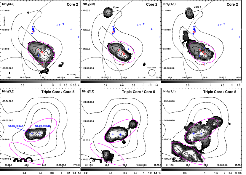
Figure 9: Intensity-weighted velocity dispersion $v_{\rm rms}$ [km s^-1] of the NH₃ (3,3), (2,2) and (1,1) emission. The (3,3) and (2,2) emission is considered over the -50 to 50 km s^-1  V_LSR range, whilst the (1,1) is considered over the 5 to 15 km s^-1  (Core 2) and 5 to 20 km s^-1  (Triple Core/Core 5) ranges to avoid the strong satellite lines contaminating the $v_{\rm rms}$ calculation. Pixel channels are masked below a $T_{\rm mb}$ value of 0.18 K ($\sim$3.5 $T_{\rm rms}$ ) threshold. Dashed black contours indicate the H.E.S.S. TeV gamma-ray significance. For Core 2 the blue/white $+$’s indicate the positions of the 1720 MHz OH masers from Claussen et al. (1999), and red $\times$’s indicate positions of broad line regions defined by Reach et al. (2005). The large and small solid circles represent the radio boundaries of the SNRs W28 and G6.67-0.42 respectively. For Triple Core/Core 5, blue/white $+$’s indicate G5.89-0.39A (Hii ) and B (UC-Hii ). The Mopra beam 2^′ FWHM is indicated on the Core 2 NH₃ (2,2) image and applies to all other images shown here. The magenta solid ellipses define regions for extended source mass and density estimates in Table 5.The implications of the more central dispersion seen in the Triple Core versus the generally asymmetric dispersion seen in Core 2 are discussed in the text.

4.4 Radiative Transfer Modeling of Core 2

The broad NH₃ (3,3) line with $\Delta v_{1/2}\sim$13 km s^-1  and its high line strength relative to (1,1) and (2,2) from Core 2 are somewhat beyond those expected from a purely thermal distribution as indicated in $\S$4.1. Such broad line profiles suggest a large amount of energy, in this case non-thermal energy from the SNR shock, has been deposited into the cloud. The velocity dispersion NH₃ (3,3) image for Core 2 (Figure 9) and the many 1720 MHz OH masers in the region indicating shocked gas support the notion that the broad NH₃ is also the result of SNR shock disruption. The analysis outlined earlier in $\S$ 4.2 for the (1,1) and (2,2) emission assumes that it comes from quiescent, cold or cool, dense cores. This assumption clearly doesn’t hold for the Core 2 region, and as such the mass and density estimates for Core 2 in Table 5 are likely underestimates which would pertain primarily to the cooler gas component. We therefore turn to more detailed radiative transfer modeling of the position-switched (1,1), (2,2), (3,3), and (6,6) spectra taken towards the peak of NH₃ (3,3) emission (Figure 8) and spectra averaged over the Core 2 region for a first look at the gas parameters towards Core 2.

The radiative transfer code, MOLLIE, can deal with arbitrary 3D geometries, but as a first step in obtaining the indicative properties of Core 2 in this paper, we modeled the emission as arising from a sphere with a constant temperature, density and non-thermal velocity component, taking the NH₃ spectra corrected for the Mopra aperture main beam efficiency of $\eta_{\rm mb}=0.6$. The NH₃  to H₂ abundance ratio was fixed at $2\times 10^{-8}$ as in our earlier analyses, and a source radius of 2.1 pc (distance 2 kpc) was chosen based on the extent of the NH₃ (3,3) intensity after a $T_{\rm mb}$ $\geq 0.18$ K cut. Models were constructed with H₂ densities, temperatures and non-thermal linewidths ranging from $10^{3}$ to $10^{8}$ cm^-3, $10$ to $400$ K and $0.5$ to $40$ km s^-1, respectively. Radiative transfer modeling was then used to generate synthetic data cubes with a velocity resolution of 0.1 km s^-1  for the NH₃ (1,1) , (2,2), (3,3) and (6,6) emission. These were then convolved with 2D Gaussian profiles at a spatial scale corresponding to the 2$\arcmin$ FWHM of Mopra. The synthetic spectra at each transition were fit to the observed spectra (weighted by the signal-to-noise of each transition) and reduced-$\chi^{2}$ values returned for the goodness-of-fit. Simulated annealing with 10,000 models was used to search through the 3D parameter space to minimise $\chi^{2}$ and find the best-fit model. This method is inherently robust against becoming trapped in local, rather than global minima in parameter space. However, to determine the robustness of the best-fit model we ran the fitting 20 times with widely separated initial start values and increments. For the position-switched spectra, the best-fit model yielded a hydrogen atom number density, temperature and non-thermal linewdith of $10^{3.45}$ cm^-3, 95 K and 7.4 km s^-1, respectively, giving a Core 2 mass of $\sim$2700 M_⊙. For the mapping-averaged spectra, the best-fit model yielded a density, temperature and non-thermal linewdith of $10^{3.12}$ cm^-3, 60 K and 7.5 km s^-1, respectively, giving a Core 2 mass of $\sim$1300 M_⊙.

Figure 10 shows the NH₃ (1,1), (2,2), (3,3) and (6,6) Mopra spectra from position-switched and averaged-mapping data overlayed with the synthetic spectra from the best-fit model. The weakly detected (9,9) spectrum was not included in both cases. Considering the simplicity of the model, the synthetic spectra match the position-switched data well. Differences between the model and data provide insight into the underlying source structure of Core 2. The single non-thermal velocity contribution to the linewidth works well for the higher transitions, but can not account for the narrow linewidth component of the NH₃ (1,1) emission from both sets of spectra used. Similarly, assuming a single temperature for Core 2 underestimates the NH₃ (6,6) emission, especially for the mapping-averaged spectra, which yield a lower density and temperature compared to position-switched results as expected. Given these issues, the Core 2 extended masses derived here are likely to be underestimates and we conservatively quote the lower of the two densities and masses in Table 5. More detailed modeling to simultaneously fit the cooler gas traced by the narrow linewidth NH₃ (1,1) emission and the hotter gas traced by the NH₃ (6,6) emission will be the focus of later work. Errors in the fitted quantities are not yet estimated due to the often imperfect fits to each spectra, and will also be discussed in later work.

Table 5: Mass $M$ and molecular hydrogen number density $n_{\rm H_{2}}$ estimates (Eqs. 3 and 4) for the various cores from $N_{\textrm{\tiny{NH}}_{3}}$ derived using NH₃ (1,1) and (2,2) parameters of Table 4. Point source analysis assumes a spherical emission volume of radius $R=0.2$ pc (with the effect of source radius scaling indicated) whilst for extended source analysis spectra are averaged over an elliptical region (see Table 4) using pixels satisfying $T_{\rm mb}$ $\geq 0.18$ K. The included range of virial masses $M_{\rm vir}$ is bounded by radial density profiles following $r^{-2}$ and Gaussian laws and assumes the NH₃ (2,2) linewidth $\Delta v_{1/2}$ (except for Core 2 which assumes the (3,3) linewidth). The radiative transfer results for Core 2 using the MOLLIE code applied to the NH₃ (1,1) to (6,6) spectra are also given.

Core Name	$M$	$n_{\rm H_{2}}$	$M_{\rm vir}$
	[M⊙]	[$10^{3}$ cm-3]	[M⊙]
—– Point Source Analysis ($R=0.2$ pc) —–
Core 1	495	287.9	220 – 760
Core 2	240	140.8	4200 – 14700$\,{}^{\dagger}$
Core 3	640	370.2	280 – 980
Core 4	190	112.3	80 – 290
Core 4a	75	43.5	230 – 810
Core 5 SW	350	202.5	140 – 480
Core 5 NE	335	196.1	100 – 360
Triple Core SE	475	276.8	330 – 1170
Triple Core Central	320	185.1	520 – 1820
Triple Core NW	130	76.7	110 – 400
Core 6	910	530.0	220 – 760
Point source mass/density scaling vs. radius $R$ (pc)
$R$ (pc)	0.10 0.15 0.20 0.25 0.30 0.35 0.40
Mass $M(R)\,/\,M(0.2{\rm pc})$	0.97 0.98 1.00 1.02 1.05 1.08 1.12
Density $n_{\rm H_{2}}(R)\,/\,n_{\rm H_{2}}(0.2{\rm pc})$	7.77 2.33 1.00 0.52 0.31 0.20 0.14
—– Extended Source Analysis —–
Core 2	1600	0.8	44400 – 152600$\,{}^{\dagger}$
Core 2 (MOLLIE)	$>$1300	$>$0.7	14500 – 51200$\,{}^{\ddagger}$
Core 5	1300	0.7	4000 – 14200
Triple Core	3300	0.5	8900 – 31400
$\dagger$ Using $\Delta v_{1/2}$ from the (3,3) emission in Table 4.
$\ddagger$ Using $\Delta v_{1/2}$ as the non-thermal line width from MOLLIE.

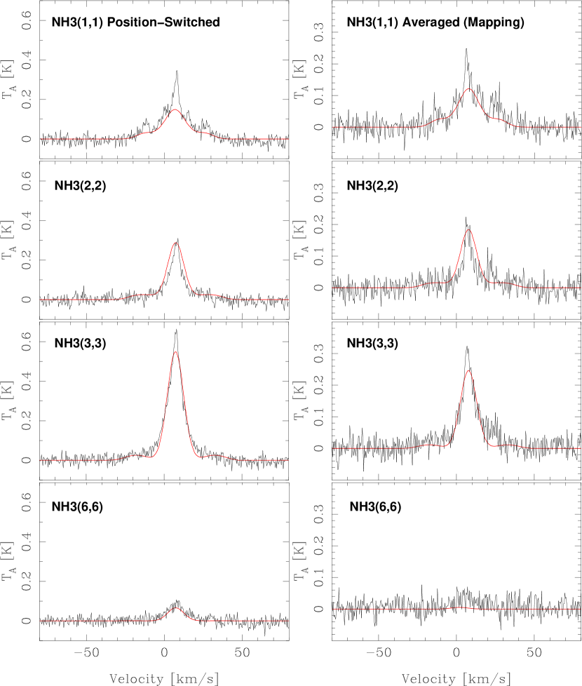
Figure 10: MOLLIE radiative transfer modeling fits to the NH₃ spectra from Core 2 outlined in $\S$4.4. Left-Column: Fits to position-switched deep spectra towards the peak NH₃ (3,3) emission. Right-Column: Fits to mapping spectra averaged over pixels with $T_{\rm mb}$ $\geq 0.18$ K. In all panels the best-fit model is overlaid as the red solid line.

5 Detailed Discussion of Cores

Core 1:

Situated at the northern boundary of HESS J1801-233 in the vicinity of the giant Hii region M20. Core 1 exhibits NH₃ (1,1), (2,2) and (3,3) emission centred at V_LSR =+21 km s^-1  with $T_{\rm k}$ $\sim 18$ K. The (1,1) and (2,2) lines are detected in mapping while the (3,3) line is only seen in the deep pointing. CS (2–1) was earlier detected at a similar V_LSR value found by Bronfman et al. (1996), who first suggested the link to the IR source IRAS 17589-2312. Based on the FIR colour ratio, these authors have also suggested IRAS 17589-2312 is indicative of an UC-Hii region. Faúndez et al. (2004) estimate a core mass of $M=210$ M_⊙, radius $\sim$0.25 pc (for 3.8 kpc distance), and density $n_{\rm H_{2}}=3.4\times 10^{4}$ cm^-3 based on their SIMBA 1.2 mm continuum mapping. Assuming a 0.25 pc radius, the mass and density estimates from our observations (500 M_⊙ and 15.0$\times 10^{4}$ cm^-3) are a factor 2 to 4 times higher than those of Faúndez et al. (2004), but in general agreement given the systematic uncertainties arising from the NH₃ abundance ratio. A similar core radius is also quoted by Lefloch et al. (2008) who studied this core using a variety of CO, CS, and HCO⁺ transitions. They suggest that star formation activity in this core is very recent which could have been triggered by the SNR W28. The H₂O maser seen towards this core has also been discussed (Codella et al., 1995).

Core 2:

As already described, Core 2 spatially coincides very well with the TeV gamma-ray source HESS J1801-233 and broad-line CO line observations (Arikawa et al., 1999; Torres et al., 2003; Reach et al., 2005; Aharonian et al., 2008b; Fukui et al., 2008). This molecular cloud is known to be shock-disrupted as evidenced by the presence of many 1720 MHz OH masers (Frail et al., 1994; Claussen et al., 1999). Further detailed studies of the shocked gas have been carried out in CO, CS and IR H₂ lines by Reach et al. (2005). Our Mopra observations reveal NH₃ inversion transitions from (1,1) up to (9,9) with very broad linewidths. The strongest emission with $\int\,\mbox{$T_{\rm mb}$\,}\,dv=\,7.4$ K km s^-1  is found in the broad $\Delta\,v_{1/2}$=12.8 km s^-1  (3,3) transition, which bears a close resemblance to the CO peaks. The velocity dispersion image of the (3,3) line in Figure 9 shows clearly that the cloud disruption originates from the western or W28 SNR side, supporting the results of Arikawa et al. (1999) who showed that the broad ¹²CO (3–2) emission is found preferentially towards the W28 side in contrast to ¹²CO (1–0) which extends radially further away. The Nanten2 ¹²CO (2–1) emission likely traces a mixture of shocked and unshocked gas and detailed velocity dispersion studies of this (2–1) emission are currently underway. The lack of strong broad-band IR features towards Core 2 (Figure 7) suggests that the NH₃ excitation is not due to star formation processes, although some fraction of the weak IR emission seen here is due to shocked H₂ (Neufeld et al., 2007; Marquez-Lugo et al., 2010). We also note there is a weak HC₃N feature seen in the deep pointing which is an indicator of hot gas-phase chemistry. It is also quite striking that a grouping of the OH masers appear to surround the region where the (3,3) emission is most disrupted (Figure 9), radially away from the W28 SNR. This would be further evidence in support of the W28 SNR as the source of molecular cloud disruption, and overall would tend to disfavour physical influence from the neighbouring SNR G6.67-0.42, which at present has an unknown distance. The broad molecular line regions discussed by Reach et al. (2005) also generally cluster towards the broadest NH₃ emission (see Figure 9).

The broadening of the NH₃ (3,3), (6,6) and probably (9,9) lines are dominated by non-thermal component(s) and we can estimate the additional kinetic energy $W_{\rm kin}$ required to achieve this from:

$$W_{\rm kin}=~{}1/2\,M\,(\Delta v_{\rm kin})^{2}$$ (7)

where $M$ is the mass of the broad-line gas and $\Delta v_{\rm kin}$ is the FWHM [m s^-1] of the line due to additional non-thermal kinetic processes. Using the non-thermal line width $\Delta v_{\rm kin}=7.5$ km s^-1  and mass lower limit $M=1300$ M_⊙ from our radiative transfer modeling in §4.4 of mapping-averaged NH₃ spectra we therefore calculate W${}_{KE}>0.7\times 10^{48}$ erg. This energy lower limit is within a factor few of the kinetic energy ($\sim\,3\times 10^{48}$ erg) deposited into the 2000 M_⊙ of gas traced by shocked ¹²CO (3–2) from Arikawa et al. 1999.

Over the 0 to 12 km s^-1  V_LSR range, for which the Nanten ¹²CO (1–0) emission shows excellent overlap with the TeV gamma-ray source HESS J1801-233, the mass of the NE molecular cloud is $\sim 2\times 10^{4}$ M_⊙. Over a wider 0 to 20 km s^-1  V_LSR range the mass is $\sim 5\times 10^{4}$ M_⊙. Thus, the $>$1300 M_⊙ of extended gas traced by our broad-line NH₃ observations represents at least 5% of the total cloud mass.

Cores 3 and 6:

Cores 3 and 6 are not found towards any of the H.E.S.S. TeV gamma-ray sources. Their V_LSR values at $\sim$-25 km s^-1  are quite different to the other Cores in the region. The most likely connection is with the near-3-kpc spiral arm (with heliocentric distance $\sim$2 to 3 kpc), which has an expected value V_LSR $=-53.1+4.16l$ [km s^-1] for Galactic longitude $l$ (see e.g. Dame et al. 2008). Core 3 is possibly associated with the B8 IV spectral type star HD 313632. Our new detection of a H₂O maser towards Core 3 may result from the envelope of HD 313632 or signal the presence of star formation. From the Spitzer image in Figure 7 a 24$\mu$m feature is seen towards this core. For Core 6, the IR and radio sources IRAS 17555-2408 and PMN J1758-2405 are found $\sim 2^{\prime}$ and $\sim 4^{\prime}$ distant. For both cores, our detection of NH₃ could signal some degree of star formation. Finally, Core 6 also lies just outside the TeV emission from HESS J1800-240C and thus is unlikely to be associated. For a 0.2 pc radius, both of these cores have masses $\sim$600 to 900 M_⊙, and densities $\sim$400 to 500$\times 10^{3}$ cm^-3.

Cores 4 and 4a

These cores are located towards the peak of the TeV gamma-ray source HESS J1800-240A and are likely associated with the Hii regions G6.225-0.569 (Core 4) and G6.1-0.6 (Core 4a) (Lockman, 1989; Kuchar & Clark, 1997). Additional counterparts to Core 4a are the IR source, IRAS 17588-2358, also clearly visible in the Spitzer image (Figure 7), and a 1612 MHz OH maser (Sevenster et al., 1997). Our detection of HC₃N(3–2) towards Core 4a may also suggest it is at an earlier evolutionary stage than Core 4. Assuming a 0.2 pc radius we derived a mass and density of 75 to 200 M_⊙ and $n_{\rm H_{2}}\sim$45 to 100$\times 10^{3}$ cm^-3 for Core 4a and Core 4 respectively. Despite the reasonable amount of clumpy molecular gas traced by Nanten CO observations (e.g. $\sim 2.5\times 10^{4}$ M_⊙ from ¹²CO (1–0) Aharonian et al. 2008b assuming a 2 kpc distance), we see no clear indication for extended NH₃ emission towards this region. We note however this region has only half the Mopra exposure compared to the other regions due to the lack of HOPS overlap.

Triple Core and Core 5

The Triple Core represents the most complex of the regions we mapped, and comprises three NH₃ peaks aligned in a SE to NW direction all of which are generally centred on the TeV gamma-ray source HESS J1800-240B and the very IR-bright and energetic Hii region G5.89-0.39. Our 12 mm observations are the largest scale mapping in dense molecular gas tracers so far of this enigmatic region. G5.89-0.39 actually comprises two active star formation sites and following the nomenclature of Kim & Koo (2001) they are labeled G5.89-0.39A to the east, and G5.89-0.39B about 2^′ to the west. The Triple Core SW NH₃ core is associated with Hii core G5.89-0.39A, otherwise known as W28-A2 after its strong radio continuum emission. The ring-like features prominently visible in the Spitzer 8$\mu$m emission (see Figure 7) are centred on G5.89-0.39A suggesting strong PAH molecular excitation from stellar photons. The Triple Core Central NH₃ core is associated with the UC-Hii region G5.89-0.39B from which strong H76$\alpha$ RRL appears to be centred (Kim & Koo, 2001) signalling strong ionisation of the surrounding molecular gas. The RRL H62$\alpha$, H65$\alpha$ and H69$\alpha$ emission from our observations also appears prominent towards G5.89-0.39B although in all three lines the emission is elongated towards G5.89-0.39A. The strongest H₂O maser is also seen towards G5.89-0.39B. From the position-switched observations, strong H₂O maser emission with complex structures spanning very wide velocity coverage over 100 km s^-1  are detected towards G5.89-0.39A and 60 km s^-1  in G5.89-0.39B. G5.89-0.39B is responsible for very energetic outflows and is extensively studied in many molecular lines over arcsec to arcmin scales. (see e.g. Harvey & Forveille 1988; Churchwell et al. 1990; Gomez 1991; Acord et al. 1997; Sollins 2004; Thompson & Macdonald 1999; Klaassen 2006; Kim & Koo 2001, 2003; Hunter et al. 2008). Previous small-scale NH₃ studies are discussed by Gomez (1991); Wood (1993); Acord et al. (1997); Hunter et al. (2008). The Triple Core NW NH₃ core is found a further 5^′ distant and may be linked to the M spectral type pulsating star V5561 Sgr or perhaps the natal gas from which this star was born.

Core 5 appears to straddle the south east quadrant of the 8$\mu$m IR shell or excitation ring of G5.89-0.39A and HESS J1800-240B, and is resolved into two components Core 5 NE and SW. Local peaks in CO emission overlapping Core 5 NE and SW are clearly visible (see Figure 6 and and also Liszt et al. (2009); Kim & Koo (2003)). Core 5 NE is the coldest of the cores detected with $T_{\rm k}$ $\sim 12$ K. Here we detect only NH₃ (1,1) emission in mapping, and only very weak (2,2) and (3,3) emission in the deep spectra. It is also one of the few sites where HC₅N(10–9) is detected. In Core 5 SW we find $T_{\rm k}$ $\sim 18$ K and NH₃ (2,2) and (3,3) emission being stronger than in the NE. There is also HC₃N(3–2) emission when looking at the 5 to 20 km s^-1  velocity range in mapping data. Overall, assuming a 0.2 pc core radius, we find our NH₃ (1,1) and (2,2) observations trace $\sim$100 to 450 M_⊙ and density $n_{\rm H_{2}}=$80 to 300$\times 10^{3}$ cm^-3 for the individual cores in the Triple Core and Core 5 complexes. The core masses are in general agreement with their virial masses.

Higher resolution NH₃ (3,3) observations of G5.39-0.39B by Gomez (1991) with the VLA suggest a 0.2 pc radius molecular envelope around G5.89-0.39B (Triple Core Central) tracing $\sim$30 M_⊙ assuming an abundance ratio ${\large\chi}_{\textrm{\tiny{NH}}_{3}}=10^{-6}$. Using our abundance ratio this mass converts to $\sim$1500 M_⊙, about a factor 5 larger than our mass estimate using the NH₃ (1,1) and (2,2) emission. This difference may arise from the fact that our analysis is not sensitive to the slightly broader (3,3) line. In addition (Purcell, 2006) estimates a core mass (for radius 0.15 pc) using SIMBA 1.2 mm continuum observations of 360 M_⊙ and derives similar virial masses from the linewidths of N₂H⁺(1–0), H¹³CO (1–0), ¹³CO (1–0) and CH₃OH transitions, which are in general agreement with our results.

Assuming the Triple Core and Core 5 complexes represent extended sources, or at least the superposition of many unresolved point sources, we derive masses and densities (Table 5) of $\sim$3300 and 1300 M_⊙ respectively with $n_{\rm H_{2}}\sim 0.7\times 10^{3}$ cm^-3 from the average NH₃ (1,1) and (2,2) emission. As for Core 2, such estimates do not consider the (3,3) emission seen towards Triple Core Central and SE and are therefore likely to underestimate the true extended mass. Nevertheless using these mass estimates the individual NH₃ cores represent about 35% of the extended mass traced by NH₃, for the two complexes, highlighting their generally clumpy nature. We also find that the extended mass traced by NH₃ represents only small fraction $\sim$5% of the total cloud mass, $\sim 0.8\times 10^{5}$ M_⊙, for the HESS J1800-240B region traced by the Nanten ¹²CO (1–0) observations over the V_LSR =0 to 20 km s^-1  range (Aharonian et al., 2008b).

An interesting question is whether or not the W28 SNR shock has reached the southern molecular clouds, as it appears to have done for Core 2 in the NE. Of interest therefore is the spatial distribution of any disruption in the molecular clouds associated with the Triple Core and Core 5 complexes. The velocity dispersion image in Figure 9 clearly shows the broader NH₃ gas is found concentrated towards the central star formation cores in constrast to Core 2 where the disruption appears to originate more from one side. As a result we would conclude there is no evidence (within the sensitivity limits of our mapping) for any external disruption of the southern molecular clouds.

6 Summary and Conclusions

We have used the Mopra 22m telescope for 12 mm line mapping over a degree-scale area covering the dense molecular gas towards the W28 SNR field. Our aim has been to probe the dense molecular cores of the gas spatially matching the four TeV gamma-ray source observed by the H.E.S.S. telescopes in this region. The wide 8 GHz bandpass of the Mopra telescopes allows to search for a wealth of molecular lines tracing dense gas. For our purpose, the empphasis has been on the inversion transitions of NH₃ which allow relatively robust estimates of gas temperature and optical depth. Our observations combine data from dedicated scans and those from the the 12 mm HOPS project and reveal dense clumpy cores of NH₃ towards most of the molecular cloud complexes overlapping the gamma-ray emission. Additional 12 mm lines were detected, including the cyanopolyynes HC₃N and HC₅N, H₂O masers, and radio recombination lines, which are prominent towards the UC-Hii complex G5.89-0.39.

The NH₃ cores are generally found in regions of ¹²CO peaks and mostly represent sites of star formation at various stages from pre-stellar cores to Hii regions. A standout exception to this is the shocked molecular cloud on the north east boundary of the W28 SNR where we detect very broad $\Delta\,v_{\rm 1/2}>10$ km s^-1  NH₃ emission up to the (9,9) transition with kinetic temperature $>$40 K. The velocity dispersion of this broad gas further supports the idea that the SNR W28 is the source of molecular disruption.

Based on analysis of the NH₃ (1,1) and (2,2) transitions we estimate total core masses for pure hydrogen in the range 75 to 900 M_⊙ assuming a core radius of 0.2 pc. Molecular hydrogen densities $n_{\rm H_{2}}$ are in the range 40 to 500$\times 10^{3}$ cm^-3, however scaling factors for various core sizes included in Table 5 indicate that density varies with core radius while mass is more robust to changes in $R$. Obviously the estimates for core masses and densities are heavily dependent on the chosen NH₃ abundance, however, the general agreement between the derived mass and virial mass for the detected cores appears to vindicate our choice of $\chi_{\textrm{\tiny{NH}}_{3}}$. Optical depths are in the range 1–4 and 0.2–1.2 for the (1,1) and (2,2) transitions respectively. The north east NH₃ core (Core 2) is extended and our radiative transfer analysis of the broad line components imply a total mass of at least 1300 M_⊙ and density $n_{\rm H_{2}}>0.7\times 10^{3}$ cm^-3. This represents $>$5% of the total north east molecular mass traced by ¹²CO (1–0) observations. For the southern molecular clouds harbouring Hii regions, the velocity dispersion centres on the individual cores (Triple Core SE/Central/NW and Core 5 NE/SW) towards the centre of the molecular clouds. Thus at this stage we find no evidence (limited by the $\sim$0.05 K per channel sensitivity of our mapping) for cloud disruption from external sources such as from W28 to the north, and thus it’s likely the W28 shock has yet to reach the southern molecular clouds. Of course this does not constrain the much faster transport of cosmic-rays from W28 to the southern clouds.

Additionally we note the densities for Core 2, Triple Core and Core 5 (Table 5) averaged over extended spherical regions are about a factor 10 below the critical density for NH₃. This would suggest that much of the cores mass is probably contained within a smaller averaged volume than that considered here, emphasising their clumpy nature. Another possible explanation for the lower densities could be the choice of spherical geometry, especially for the Core 2 region it is plausible that the shock has compressed the core deforming its geometry.

This work is part of our ongoing study into the molecular gas towards the W28 region, and help to further understand internal structures and dynamics of the molecular gas in the W28 SNR field. Deeper observations in 2010 reaching a $\sim$0.02 K channel sensitivity in the NH₃ (1,1) to (6,6) (including (4,4)) transitions, have been made with Mopra in 12 mm towards the NE (Core 2). These deep observations will permit pixel-by-pixel determination of gas parameters such as density, temperature and line width. They will therefore permit a much more detailed probe of the effects of the SNR shock propagating into the Core 2 cloud, using theoretical predictions of the effects of shocks in molecular clouds (Hollenbach & McKee, 1979; Draine et al., 1983; Hollenbach & McKee, 1989). Additionally, we recently completed a survey in the 7 mm band to trace the disrupted and shocked gas with the SiO (1–0) and CS (1–0) lines. Finally, we would also add that deeper gamma-ray observations of the W28 sources will allow higher resolution gamma-ray imaging approaching the molecular core sizes revealed in this study. This, when combined with knowledge of molecular cloud structures on arcminute scales, will pave the way to probe the diffusion properties of cosmic-rays potentially producing the TeV gamma-ray emission.

References

- Abdo et al. (2010) Abdo A. et al (Fermi Collab.) 2010, ApJ submitted arXiv:1005.4474.
- Acciari et al. (2009) Acciari V. et al. 2009, ApJ, 698, L133.
- Acord et al. (1997) Acord, J., Walmsley, C. & Churchwell, E. 1997, ApJ, 475, 693.
- Arikawa et al. (1999) Arikawa, Y., Tatematsu, K., Sekimoto, Y. & Takaashi, T. 1999, PASJ, 51, L7.
- Aharonian et al. (2004) Aharonian, F., Akhperjanian, A., Aye, K. et al. (H.E.S.S. Collab.) 2004, A&A, 425, L13.
- Aharonian at al. (2006) Aharonian, F., Akhperjanian, A., Bazer-Bachi, A. et al. (H.E.S.S. Collab.) 2006, Nature, 439, 695.
- Aharonian et al. (2008a) Aharonian, F., Akhperjanian, A., Barres de Almeida, U. et al. (H.E.S.S. Collab.) 2008a, A&A, 490, 685.
- Aharonian et al. (2008b) Aharonian, F., Akhperjanian, A., Bazer-Bachi A. et al. (H.E.S.S. Collab.) 2008b, A&A, 481, 401.
- Albert et al. (2008) Albert J., Aliu E., Anderhub H. et al. (MAGIC Collab.) 2008, ApJ, 674, 1037.
- Araudo et al. (2007) Araudo A., Romero, G., Bosch-Ramon, V. & Parades J. 2007, A&A, 476, 1289.
- Barrett et al. (1977) Barrett, A., Ho, P., Myers, P. 1977, ApJ, 211, L39.
- Brogan et al. (2006) Brogan, C., Gelfand, J., Gaensler, B. et al. 2006, ApJ, 639, L25.
- Bergin et al. (2006) Bergin, E., Maret, S., van der Tak, F. et al. 2006, ApJ, 645, 369.
- Breen et al. (2009) Breen, S., Ellingsen, S., Caswell, J. & Lewis, B. 2010, MNRAS, 401, 2219.
- Bronfman et al. (1996) Bronfman L., Nyman L.-øA., May J. 1996, A&AS, 115, 81.
- Chapmann et al. (2009) Chapmann, J., Miller, T., Wardle, M. et al. 2009, MNRAS, 394, 221.
- Churchwell et al. (1990) Churchwell, E., Walmsley, C., Cesaroni, R. 1990, A&A SS, 83, 199.
- Claussen et al. (1999) Claussen, M., Goss, W., Frail, D. & Desai, K. 1999, ApJ, 522, 349.
- Codella et al. (1995) Codella C., Palumbo G.G.C., Pareschi G. et al. 1995, MNRAS, 276, 57.
- Dubner et al. (2000) Dubner G., Velázquez P., Goss W., Holdaway M. 2000, AJ 120, 1933.
- Dame et al. (2001) Dame, T., Hartmann, D. & Thaddeus, P. 2001, ApJ, 547, 792.
- Dame et al. (2008) Dame, T., Thaddeus, P. 2008, ApJ, 683, L143.
- Draine et al. (1983) Draine, B. T., Roberge, W. G. & Dalgarno, A. 1983, ApJ, 264, 485.
- Faúndez et al. (2004) Faúndez S., Bronfman L., Garay G. et al. 2004, A&A, 426, 97.
- Feinstein et al. (2009) Feinstein F., Fiasson A., Gallant Y. et al. 2009, AIP Conf. Proc. 1112, 54.
- Frail et al. (1994) Frail, D., Goss, W., Slysh, V. 1994, ApJ, 424, L111.
- Fujita et al. (2009) Fujita Y., Ohira Y., Tanaka S., Takahara F. 2009, ApJ, 707, L179.
- Fukui et al. (2008) Fukui, Y. et al., 2008, AIP Conf. Proc., 1085, 104.
- Gabici et al. (2007) Gabici, S., Aharonian, F. & Blasi, P. 2007, Astrophys. Space Sci., 309, 365.
- Giuliani et al. (2010) Giuliani A., Tavani M., Bulgarelli A. et al. 2010, ApJ A&A, 516, L11.
- Goldsmith & Langer (1999) Goldsmith, P. & Langer W. 1999, ApJ, 517, 209.
- Gomez (1991) Gómez Y., Rodríguez L.F., Garay G., Moran J.M. 1991, ApJ, 377, 519.
- Goudis (1976) Goudis C 1976, Ap&SS, 40, 91.
- Harvey & Forveille (1988) Harvey, P. & Forveille, T. 1988, A&A, 197, L19.
- Hewitt & Yusef-Zadeh (2009) Hewitt, J., Yusef-Zadeh, F. 2009, ApJ, 694, L16.
- Ho & Townes (1983) Ho, P. & Townes, C. 1983, Ann. Rev. Astron. Astrophysics, 21, 239.
- Hollenbach & McKee (1979) Hollenbach, D. & McKee, C. F. 1979, ApJSS, 41, 555.
- Hollenbach & McKee (1989) Hollenbach, D. & McKee, C. F. 1989, ApJ, 342, 306.
- Hunter et al. (2008) Hunter T.L., Brogan C.L., Indebetouw R., Cyganowski C.J. 2008, ApJ, 680, 1270.
- Johnston et al. (1973) Johnston K.J., Sloanaker R.M., Bologna J.M. 1973, ApJ, 182, 67.
- Kaspi et al. (1993) Kaspi V., Lyne A., Manchester R. et al. 1993, ApJ, 409, L57.
- Keto (1990) Keto, E. 1990, ApJ, 355, 190.
- Keto et al. (2004) Keto, E., Rybicki, G. B., Bergin, E. A., & Plume, R. 2004, ApJ, 613, 355.
- Keto & Zhang (2010) Keto, E. & Zhang, Q. 2010, MNRAS, 406, 102.
- Kim & Koo (2001) Kim K., Koo B. 2001, ApJ, 549, 979.
- Kim & Koo (2003) Kim K., Koo B. 2003, ApJ, 596, 362.
- Klaassen (2006) Klaassen P.D., Plume R., Ouyed R. et al. 2006, ApJ, 648, 1079.
- Kuchar & Clark (1997) Kuchar T.A., Clark F.O. 1997, ApJ, 488, 224.
- Lefloch et al. (2008) Lefloch B., Cernicharo J., Pardo J.R. 2008, A&A, 489, 157.
- Liszt et al. (2009) Liszt H.S. 2009, A&A 508, 1331.
- Lockman (1989) Lockman F.J. 1989, ApJS, 71, 469.
- Longmore et al. (2010) Longmore, S., Pillai, T., Keto, E., Zhang, Q., & Qi, K. 2010, ApJ in press.
- Lozinskaya (1981) Lozinskaya T.A. 1981, Sov. Astron. Lett., 7, 17.
- MacLaren (1988) MacLaren I., Richardson K.M., Wolfendale A.W. 1988, ApJ, 333, 821.
- Marquez-Lugo et al. (2010) Marquez-Lugo R.A, & Phillips J. P. 2010, MNRAS, 407, 94.
- Mizuno & Fukui (2004) Mizuno, A. & Fukui, Y. 2004, AIP Conf. Proc., 317, 59.
- Neufeld et al. (2007) Neufeld D.A., Hollenbach D.J., Kaufman M.J. et al. 2007, ApJ 664, 890.
- Ott et al. (2005) Ott, J., Weiß, A., Henkel, C. & Walter, F. 2005, ApJ, 629, 767.
- Ott et al. (2010) Ott, J., Henkel C., Staveley-Smith L., Weiss A. 2010, ApJ 710, 105.
- Pillai et al. (2006) Pillai, T., Wyrowski, F., Carey, S. & Menten, K. 2006, A&A, 450, 569.
- Protheroe et al. (2008) Protheroe R.J., Ott J., Ekers R.D. et al. 2008, MNRAS, 390, 683.
- Purcell (2006) Purcell, C. PhD Thesis, What’s in the brew? A study of the molecular environment of methanol masers and UCHII regions, UNSW, 2006.
- Reach et al. (2000) Reach W., Rho J. 2000, ApJ 544, 843.
- Reach et al. (2005) Reach W., Rho J., Jarrett T. 2005, ApJ 618, 297.
- Rho & Borkowski (2002) Rho, J. & Borkowski, K. 2002, ApJ, 575, 201.
- Sollins (2004) Sollins P.K., Hunter T.R., Battat J. et al. 2004, ApJ, 616, L35.
- Sevenster et al. (1997) Sevenster M.N., Chapman J.M, Habing H.J. et al. 1997, A&A Supp, 122, 79.
- Stahler & Palla (2005) Stahler, S. & Palla, F. The Formation of Stars, 2005.
- Suzuki et al. (1992) Suzuki, H., Yamamoto, S., Ohishi, M. et al. 1992, ApJ, 392, 551.
- Tafalla et al. (2004) Tafalla, M., Myers, P., Caselli, P. & Walmsley, C. 2004, A&A, 416, 191.
- Thompson & Macdonald (1999) Thompson M.A., Macdonald G.H. 1999, A&A(Supp), 135, 531.
- Torres et al. (2003) Torres D., Romero G., Dame T. et al. 2003, Phys. Rep. 382, 303.
- Ungerechts et al. (1986) Ungerechts, H., Walmsley, C. & Winnewisser, G. 1986, A&A, 157, 207.
- Urquhart et al. (2010) Urquhart J.S., Hoare M.G., Purcell C.R. et al. 2010, PASA, 27, 321.
- Velázquez et al. (2010) Velázquez P.F., Dubner G.M., Goss W.M., Green A.J. 2002, AJ 124, 2145.
- Walmsley & Schilke (1983) Walmsley, M. & Schilke, P. 1983, Dust and Chemistry in Astronomy, 37.
- Walmsley & Schilke (1992) Walmsley, M. & Schilke, P. 1992, Hot cores and cold grains in: Astrochemistry of cosmic phenomena, IAU symposium 150.
- Walsh et al. (2008) Walsh, A., Lo, N., Burton, M. et al. 2008, PASA, 25, 105.
- Wood (1993) Wood D.O.S. 1993, ASP Conf. Ser. 35, 108.
- Yusef-Zadeh et al. (2000) Yusef-Zadeh, F., Shure, M., Wardle, M. & Kassim, N. 2000, ApJ, 540, 842.