Spectral dependence of photoinduced spin precession in DyFeO₃

Abstract

Spin precession was nonthermally induced by an ultrashort laser pulse in orthoferrite DyFeO₃ with a pump–probe technique. Both circularly and linearly polarized pulses led to spin precessions; these phenomena are interpreted as the inverse Faraday effect and the inverse Cotton–Mouton effect, respectively. For both cases, the same mode of spin precession was excited; the precession frequencies and polarization were the same, but the phases of oscillations were different. We have shown theoretically and experimentally that the analysis of phases can distinguish between these two mechanisms. We have demonstrated experimentally that in the visible region, the inverse Faraday effect was dominant, whereas the inverse Cotton–Mouton effect became relatively prominent in the near-infrared region.

I INTRODUCTION

Magnetization switching triggered by femtosecond laser pulses has been studied in recent years. Ultrafast demagnetization in ferromagnetic metals and semiconductors has also been reported.Beaurepaire ; Wang These phenomena show thermal magnetic switching with light pulses on picosecond time scales.Koopmans However, heat-assisted spin reorientation is relatively slow because of the thermal diffusion time.

A light pulse with a certain polarization nonthermally modifies the electron spin state.Ju ; Dalla Recently, it has been reported that spin precession is induced by a circularly polarized pulse in antiferromagnetic (AFM) DyFeO₃ with weak ferromagnetic (FM) moment.Kimel1 The phase of spin precession changes by 180^∘ on reversal of the pump helicity. The interpretation of this phenomenon is that an effective magnetic field pulse parallel to the pump wave vector is induced by the circularly polarized light pulse, giving rise to the precession. The magnetic field generation effect is referred to as the inverse Faraday effect (IFE). The same effect has also been observed even in pure AFM NiO with no net magnetic moment in the ground state.Satoh1 The resonance frequencies of AFM materials reach the terahertz range, which is several orders of magnitude higher than that of FM materials. For that reason, AFM materials attract much attention in the context of ultrafast spin control.Satoh1 ; Dodge ; Kimel2 ; Zhao ; Kimel3 ; Nishitani ; Yamaguchi ; Kampfrath ; Higuchi Spin precession is also observed with a linearly polarized pump pulse, in particular, a pulse polarized in a direction non-parallel to the crystal axes. This phenomenon is called the inverse Cotton–Mouton effect (ICME).Kalashnikova1 ; Kalashnikova2 A detailed review of these phenomena can be found in Ref. Kirilyuk+RMPh, .

The ultrafast IFE and ICME are interpreted as impulsive stimulated Raman scattering (ISRS).Kimel4 ; Yan ; Merlin An electron in the ground state is excited by the pump pulse into a virtual state, which changes the orbital momentum of the electron. The nonzero orbital momentum flips the electron spin with spin-orbit coupling in the virtual state. The excited electron radiates a photon and transits to the final state. The energy gap between the final and ground states corresponds to the spin precession energy.

ISRS is a modulation of the dielectric permittivity by the pump pulse and should be dependent on the properties of the pulse, such as its polarization, wavelength, and fluence. Therefore, examining the dependence of the photoinduced spin precession on these properties will help us to understand the ISRS mechanism. In particular, it is not obvious how the pump photon energy influences spin precession. An action spectrum of photoinduced spin precession should indicate the relation between the optical excited state and the spin precession via ISRS.

In the majority of previous publications, the excitation of spin oscillations by ultrashort laser pulses was associated with IFE and ICME separately. In the present work, we report spin precession induced via ISRS as functions of the pump pulse polarization and wavelength. We found that both effects, IFE and ICME are working in the same way, exciting the same mode of spin precession. The phases of the spin precession via IFE and ICME differ by 90^∘, allowing the two effects to be distinguished. We found an essential dependence of the phase on the pump wavelength and demonstrated that the IFE and ICME are dominating effects in different spectral regions, in the visible region and in the near-infrared region, respectively. Thus, the analysis of the phase difference of the spin precession reveals the mechanism of ISRS.

II PHYSICAL PROPERTIES

II.1 Crystallographic and magnetic properties

DyFeO₃ is a rare-earth orthoferrite and crystallizes in an orthorhombic structure $D^{16}_{2h}$ $(Pbnm)$.Wijn Spins of the Dy³⁺ ions are not ordered above 4 K. Four Fe³⁺ ions occupy positions (1/2, 0, 0), (1/2, 0, 1/2), (0, 1/2, 1/2), and (0, 1/2, 0) in the unit cell. In the exchange approximation, the arrangement of their magnetic moments, $\textbf{{M}}_{1}$, $\textbf{{M}}_{2}$, $\textbf{{M}}_{3}$, $\textbf{{M}}_{4}$, corresponds to one of the four patterns $G_{i}:M_{1i}=-M_{2i}=M_{3i}=-M_{4i}$, $F_{i}:M_{1i}=M_{2i}=M_{3i}=M_{4i}$, $A_{i}:M_{1i}=-M_{2i}=-M_{3i}=M_{4i}$, and $C_{i}:M_{1i}=M_{2i}=-M_{3i}=-M_{4i}$ $(i=x,$ $y,$ $z)$. DyFeO₃ crystal has the spin arrangement $\Gamma_{4}(G_{x}A_{y}F_{z})$ and belongs to the magnetic point group $m^{\prime}m^{\prime}m$ above the Morin point and below the Néel temperature, at 37 K $<T<$ $T_{N}=645$ K.Gorodetsky ; Tokunaga ; Baryakhtar ; Treves ; White1 Because of the superexchange interaction, the spins are almost completely arranged antiferromagnetically along the $x$-axis. Due to the Dzyaloshinskii–Moriya interaction, all spins tilt by about $0.5^{\circ}$ toward the $z$-axis.Dzyaloshinskii ; Moriya Usually the conditions $\textbf{{M}}_{1}\sim\textbf{{M}}_{3}$ and $\textbf{{M}}_{2}\sim\textbf{{M}}_{4}$ are valid and a simpler model with just two different sublattice magnetic moments, $\textbf{{M}}_{1}$ and $\textbf{{M}}_{2}$, with $|\textbf{{M}}_{1}|=|\textbf{{M}}_{2}|=M_{0}$, can be employed.Baryakhtar ; Herrmann In what follows, this two-sublattice model will be used. We denote the FM vector by $\textbf{{M}}=\textbf{{M}}_{1}+\textbf{{M}}_{2}$ and the AFM vector by $\textbf{{L}}=\textbf{{M}}_{1}-\textbf{{M}}_{2}$. These vectors are subject to constraints

$$(\textbf{{M}}\cdot\textbf{{L}})=0,\ \textbf{{M}}^{2}+\textbf{{L}}^{2}=4M_{0}^{2}.$$ (1)

The dynamics of $\textbf{{M}}(t)$ and $\textbf{{L}}(t)$ is described by Landau–Lifshitz equationsBaryakhtar ; Balbashov ; Turov1

$$\frac{d\textbf{{M}}(t)}{dt}=-\gamma\{[\textbf{{M}}(t)\times\textbf{{H}}^{\rm{eff}}]+[\textbf{{L}}(t)\times\textbf{{h}}^{\rm{eff}}]\},$$ (2)

$$\frac{d\textbf{{L}}(t)}{dt}=-\gamma\{[\textbf{{M}}(t)\times\textbf{{h}}^{\rm{eff}}]+[\textbf{{L}}(t)\times\textbf{{H}}^{\rm{eff}}]\},$$ (3)

where $\gamma=g\mu_{\mathrm{B}}/\hbar$ ($>0$) is the gyromagnetic constant, $\mu_{\mathrm{B}}$ is the modulus of the Bohr magneton, $g$ is the gyromagnetic ratio, $g\approx 2$ for orthoferrites, and $\textbf{{H}}^{\rm{eff}}$ and $\textbf{{h}}^{\rm{eff}}$ are the effective magnetic fields. Using the magnetic energy of an orthoferrite, the effective fields are denoted as $\textbf{{H}}^{\rm{eff}}=-\partial\mathcal{H}/\partial\textbf{{M}}$ and $\textbf{{h}}^{\rm{eff}}=-\partial\mathcal{H}/\partial\textbf{{L}}$, where the Hamiltonian is given byTurov2 ; Baryakhtar

$$\mathcal{H}=\frac{A}{2}\textbf{{M}}^{2}+\frac{p_{1}}{2}M_{x}^{2}+\frac{p_{3}}{2}M_{z}^{2}+\frac{q_{1}}{2}L_{x}^{2}+\frac{q_{3}}{2}L_{z}^{2}-\textbf{{d}}\cdot(\textbf{{M}}\times\textbf{{L}}).$$ (4)

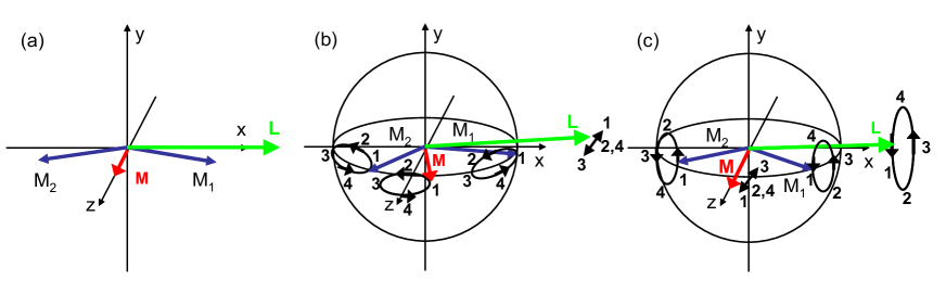
Figure 1: (a) The static magnetic structure of DyFeO₃, with the four Fe³⁺ spins regarded as satisfying $\textbf{{M}}_{1}\simeq\textbf{{M}}_{3}$ and $\textbf{{M}}_{2}\simeq\textbf{{M}}_{4}$. (b) Quasi-ferromagnetic and (c) quasi-antiferromagnetic spin precession.

The last term describes the Dzyaloshinskii–Moriya interaction and d is parallel to the $y$-axis. Equations (2), (3), linearized above the ground state determined by the energy (4), yield eigenmodes of oscillations of the vectors $\textbf{{M}}(t)$ and $\textbf{{L}}(t)$. These spin precession modes for the $\Gamma_{4}$ ground state with the equilibrium values of $M_{z}\neq 0$ and $L_{x}\neq 0$ (see Fig. 1(a)) are described as follows

with as following:

$$\textbf{{M}}(t)=M_{z}\hat{\textbf{z}}+\textbf{{m}}(t),$$ (5)

$$\textbf{{L}}(t)=L_{x}\hat{\textbf{x}}+\textbf{{l}}(t).$$ (6)

where $\hat{\textbf{z}}$ and $\hat{\textbf{x}}$ are unit vectors parallel to the $z$-axis and $x$-axis, respectively, and the variables $\textbf{{m}}(t)$ and $\textbf{{l}}(t)$ correspond to two eigenfrequency modes, as shown in Fig. 1(b) and (c). The components $m_{x}$, $m_{y}$ and $l_{z}$ oscillate at the quasi-ferromagnetic resonance (F-mode) with the angular frequency $\omega_{\rm F}$. On the other hand, $l_{x}$, $l_{y}$, and $m_{z}$ oscillate at the quasi-antiferromagnetic resonance (AF-mode) with the angular frequency $\omega_{\rm AF}$.Herrmann Those resonance frequencies are given byTurov2 ; Cinader ; Koshizuka

$$\omega_{\rm F}=2\gamma M_{0}\sqrt{A(q_{3}-q_{1})},$$ (7)

$$\omega_{\rm AF}=2\gamma M_{0}\sqrt{d^{2}-Aq_{1}},$$ (8)

where $M_{0}=|\textbf{{M}}_{1}|=|\textbf{{M}}_{2}|$, and the anisotropy constants $p_{1}$ and $p_{3}$ are omitted, because their contribution to frequencies is negligible. (It is worth to note here, that the exchange-relativistic constant of the Dzyaloshinskii–Moriya interaction has the same order of magnitude as a square root of the product of exchange and relativistic constants like $\sqrt{A|q_{1}|}$ and thus should be kept in the above expressions.) The orbits of the spin precession and the temporal response of M and L are different in the two modes.

II.2 Optical and magneto-optical properties

DyFeO₃ has the d-d transitions ${}^{6}A_{1g}\rightarrow$ ${}^{4}E_{g},$ ${}^{4}A_{1g}$ centered at the wavelength of 500 nm, ${}^{6}A_{1g}\rightarrow$ ${}^{4}T_{2g}$ at 700 nm, and ${}^{6}A_{1g}\rightarrow$ ${}^{4}T_{1g}$ at 1000 nm.Wood ; Kahn This crystal is optically biaxial, so the components of the dielectric permittivity tensor are $\varepsilon_{xx}^{0}\not=\varepsilon_{yy}^{0}\not=\varepsilon_{zz}^{0}$. The birefringence $\rho$ stems from the difference in the refractive indices, such as $\Delta n_{xy}=n_{x}-n_{y}$ $(\rho=2\pi\Delta n/\lambda)$. On the other hand, the magnetization $M_{z}$ leads to the Faraday rotation for the light propagating along the $z$-axis. The Faraday effect is much smaller than the effect of birefringence. In DyFeO₃, the Faraday rotation $\phi$ and the birefringence per unit length are $\phi=1.6\times 10^{3}$ deg/cm and $\rho=1.2\times 10^{5}$ deg/cm, respectively, at 800 nm.Tabor1 ; Chetkin ; Tabor2

II.3 Interaction of the light pulse and the medium

The interaction of the magnetic medium and transmitting light is described by the dielectric permittivity tensor $\varepsilon_{ij}$.Smolenskii ; LL_book By virtue of the Onsager principle, if absorption is negligible, $\varepsilon_{ij}$ can be divided into antisymmetric and symmetric parts, $(\varepsilon_{ij}^{a}=-\varepsilon_{ji}^{a})$ and $(\varepsilon_{ij}^{s}=\varepsilon_{ji}^{s})$, with real and imaginary components, respectively. For a transparent medium, the tensor components can be written in the following general form

$$\varepsilon_{ij}=\varepsilon_{ij}^{(0)}+if_{ijk}M_{k}+ig_{ijk}L_{k}+a_{ijkl}M_{k}M_{l}+b_{ijkl}L_{k}L_{l}+c_{ijkl}M_{k}L_{l},$$ (9)

where $\varepsilon_{ij}^{(0)}$ is a magnetization-independent term having a symmetric part only. By taking into account the symmetry of orthoferrite, the terms in the first line (except the $\varepsilon_{ij}^{(0)}$) represent the antisymmetric part of $\varepsilon_{ij}$, and the terms in the second line describe the spin-dependent symmetric part of the permittivity tensor. The symmetry of the fourth rank tensors $a_{ijkl}$, $b_{ijkl}$, and $c_{ijkl}$ is determined by the magnetic and crystal point groups, and $f_{ijk}$ and $g_{ijk}$ are the third rank tensors, antisymmetric over the first pair of indices, e.g., $f_{ijk}=-f_{jik}$. Tensors $c_{ijkl}$ and $g_{ijk}$ originate from the Dzyaloshinskii–Moriya interaction. The Hamiltonian of the interaction between the light pulse and the medium in SI unit isLL_book

$$\mathcal{H}_{\rm int}=\frac{\varepsilon_{ij}}{4}\mathcal{E}_{i}(t)\mathcal{E}_{j}^{*}(t),$$ (10)

where $\mathcal{E}_{i}(t)$ is the time-dependent amplitude of the light in the pulse. A circularly polarized pulse propagating along the $z$-axis can be described in the form $(\mathcal{E}_{x}(t),\mathcal{E}_{y}(t))=\frac{\mathcal{E}(t)}{\sqrt{2}}(1,\pm i)$, where the $\pm$ indicate the opposite senses of helicity. A linearly polarized pulse with the polarization inclined on at an angle $\theta$ with respect to the $x$-axis can be described in the form $(\mathcal{E}_{x}(t),\mathcal{E}_{y}(t))=\mathcal{E}(t)(\cos\theta,\sin\theta)$. Then a straightforward calculation gives the Hamiltonian of the interaction with the medium of the form

$$\mathcal{H}_{\rm int}^{\sigma^{\pm}}=\frac{1}{8}\mathcal{E}(t)\mathcal{E}^{*}(t)\left(\varepsilon_{xx}^{s}+\varepsilon_{yy}^{s}\mp 2i\varepsilon_{xy}^{a}\right),$$ (11)

$$\mathcal{H}_{\rm int}^{\rm lin}=\frac{1}{4}\mathcal{E}(t)\mathcal{E}^{*}(t)\left(\varepsilon_{xx}^{s}\cos^{2}\theta+\varepsilon_{yy}^{s}\sin^{2}\theta+\varepsilon_{xy}^{s}\sin 2\theta\right),$$ (12)

for circularly and linearly polarized pulses, respectively. Nonzero components of the tensors $\varepsilon_{ij}^{s}$ and $\varepsilon_{ij}^{a}$ are listed in Table 1.Eremenko ; Zyezdin

When a pulse is incident on a medium, the interaction between the pulse and the medium is given by Eqs. (10)–(12).

Table 1: The dielectric permittivity tensor $\varepsilon_{ij}$ as a function of magnetic component. Modulation of the dielectric permittivity in F-mode and AF-mode is shown in columns 3 and 4, respectively. No external magnetic field is present. $\varepsilon_{ij}^{a}=-\varepsilon_{ji}^{a}$ and $\varepsilon_{ij}^{s}=\varepsilon_{ji}^{s}$

Tensor	Static	F-mode	AF-mode
element	(m(t)=0, l(t)=0)	($m_{x},m_{y},l_{z}\not=0$)	($l_{x},l_{y},m_{z}\not=0$)
$\varepsilon_{xx}^{s}$	$a_{xxzz}M_{z}^{2}+b_{xxxx}L_{x}^{2}$	0	$(2a_{xxzz}M_{z}+c_{xxzx}L_{x})m_{z}$
	$~{}~{}~{}~{}~{}~{}~{}~{}~{}+c_{xxzx}M_{z}L_{x}$		$~{}~{}~{}+(2b_{xxxx}L_{x}+c_{xxzx}M_{z})l_{x}$
$\varepsilon_{yy}^{s}$	$a_{yyzz}M_{z}^{2}+b_{yyxx}L_{x}^{2}$	0	$(2a_{yyzz}M_{z}+c_{yyzx}L_{x})m_{z}$
	$~{}~{}~{}~{}~{}~{}~{}~{}~{}+c_{yyzx}M_{z}L_{x}$		$~{}~{}~{}+(2b_{yyxx}L_{x}+c_{yyzx}M_{z})l_{x}$
$\varepsilon_{zz}^{s}$	$a_{zzzz}M_{z}^{2}+b_{zzxx}L_{x}^{2}$	0	$(2a_{zzzz}M_{z}+c_{zzzx}L_{x})m_{z}$
	$~{}~{}~{}~{}~{}~{}~{}~{}~{}+c_{zzzx}M_{z}L_{x}$		$~{}~{}~{}+(2b_{zzxx}L_{x}+c_{zzzx}M_{z})l_{x}$
$\varepsilon_{xy}^{s}$	0	0	$(2b_{xyxy}L_{x}+c_{xyzy}M_{z})l_{y}$
$\varepsilon_{zx}^{s}$	0	$(2a_{zxxz}M_{z}+c_{zxxx}L_{x})m_{x}$	0
		$~{}~{}~{}+(2b_{zxxz}L_{x}+c_{zxzz}M_{z})l_{z}$
$\varepsilon_{yz}^{s}$	0	$(2a_{yzyz}M_{z}+c_{yzyx}L_{x})m_{y}$	0
$\varepsilon_{xy}^{a}$	$if_{xyz}M_{z}+ig_{xyx}L_{x}$	0	$if_{xyz}m_{z}+ig_{xyx}l_{x}$
$\varepsilon_{zx}^{a}$	0	$if_{zxy}m_{y}$	0
$\varepsilon_{yz}^{a}$	0	$if_{yzx}m_{x}+ig_{yzz}l_{z}$	0

The incident pump pulse generates effective pulsed fields $\textbf{{H}}^{\rm{eff}}=-\partial\mathcal{H}_{\rm int}/\partial\textbf{{M}}$ and $\textbf{{h}}^{\rm{eff}}=-\partial\mathcal{H}_{\rm int}/\partial\textbf{{L}}$. Both effective fields are proportional to the intensity of the light, $\mathcal{E}(t)\mathcal{E}^{*}(t)$. If the pulse duration $\Delta$ is much shorter than the period of spin oscillations, $\Delta\ll 1/\omega_{\rm F},1/\omega_{\rm AF}$, the real pulse shape can be replaced by the Dirac delta function, $\mathcal{E}(t)\mathcal{E}^{*}(t)\to I_{0}\delta(t)$, where $I_{0}=\int\mathcal{E}(t)\mathcal{E}^{*}(t)dt$ is the integrated pulse intensity. The light-induced effective fields $\textbf{{H}}^{\rm{eff}}$ and $\textbf{{h}}^{\rm{eff}}$ can be regarded as being proportional to the delta function $\delta(t)$ as well. For a light pulse propagating along the $z$-axis, $\textbf{{H}}^{\rm{eff}}$ and $\textbf{{h}}^{\rm{eff}}$ generated by a circularly polarized pulse are

$$\textbf{{H}}^{{\rm eff,}\sigma^{\pm}}=-\frac{I_{0}\delta(t)}{8}[2(a_{xxzz}+a_{yyzz})M_{z}+(c_{xxzx}+c_{yyzx})L_{x}\pm 2f_{xyz}]\hat{\mathbf{z}},$$ (13)

$$\textbf{{h}}^{{\rm eff,}\sigma^{\pm}}=-\frac{I_{0}\delta(t)}{8}[2(b_{xxxx}+b_{yyxx})L_{x}\\ +(c_{xxzx}+c_{yyzx})M_{z}\pm 2g_{xyx}]\hat{\mathbf{x}},$$ (14)

respectively. The phenomenon of generating these effective magnetic fields is known as IFE.

For a magnetic field pulse of a short duration, the action of the light-induced effective fields within the delta-function approximation can be described as an instantaneous deviation of the FM and AFM vectors, $\Delta\textbf{{M}}=\textbf{{M}}(t=+0)-\textbf{{M}}(t=-0)$ and $\Delta\textbf{{L}}=\textbf{{L}}(t=+0)-\textbf{{L}}(t=-0)$, from their equilibrium positions, $\textbf{{M}}(t=-0)=M_{z}\hat{\mathbf{z}}$ and $\textbf{{L}}(t=-0)=L_{x}\hat{\mathbf{x}}$, respectively. After vanishing of the pulsed effective field, the spins precess around the effective fields corresponding to their equilibrium directions following the Landau–Lifshitz equations, based on the Hamiltonian (4). Thus the action of the pulse can be regarded as a creation of some (non-equilibrium) initial conditions for the Landau–Lifshitz equations. The deviation of the FM and AFM vectors induced by the circularly polarized pulse is described by

$$\Delta\textbf{{M}}^{\sigma^{\pm}}=0,$$ (15)

$$\Delta\textbf{{L}}^{\sigma^{\pm}}=-\frac{\gamma I_{0}}{8}[2(b_{xxxx}+b_{yyxx}-a_{xxzz}-a_{yyzz})M_{z}L_{x}+(c_{xxzx}+c_{yyzx})M_{z}^{2}\\ -(c_{xxzx}+c_{yyzx})L_{x}^{2}\mp 2(f_{xyz}L_{x}-g_{xyx}M_{z})]\hat{\mathbf{y}}.$$ (16)

Here, M is not affected by the effective field directly, whereas $l_{y}$ of $\textbf{{L}}(t)$ takes nonzero deviations. The resonance mode with $l_{y}\not=0$ is AF-mode. In Fig. 1(c), two spins $\textbf{{M}}_{1}$ and $\textbf{{M}}_{2}$, as well as their sum and difference M and L, move toward positions 2 or 4, and the spins precess around their ground state directions. Because the spins have only an $l_{y}$ variable component when the effective magnetic field disappears, spin precession starts at position 2 or 4 (see Fig. 1(c)).

Similarly, effective magnetic fields induced by a linearly polarized pulse are

$$\textbf{{H}}^{\rm eff,lin}=-\frac{I_{0}\delta(t)}{4}[(2a_{xxzz}M_{z}+c_{xxzx}L_{x})\cos^{2}\theta\\ +(2a_{yyzz}M_{z}+c_{yyzx}L_{x})\sin^{2}\theta]\hat{\mathbf{z}},$$ (17)

$$\textbf{{h}}^{\rm eff,lin}=-\frac{I_{0}\delta(t)}{4}[\{(2b_{xxxx}L_{x}+c_{xxzx}M_{z})\cos^{2}\theta+(2b_{yyxx}L_{x}+c_{yyzx}M_{z})\sin^{2}\theta\}\hat{\mathbf{x}}\\ +(2b_{xyxy}L_{x}+c_{xyzy}M_{z})\sin 2\theta\cdot\hat{\mathbf{y}}].$$ (18)

These effective magnetic fields are induced via ICME. The deviations of the FM and AFM vectors created by the effective field are

$$\Delta\textbf{{M}}^{\rm lin}=\frac{\gamma I_{0}}{4}(2b_{xyxy}L_{x}^{2}+c_{xyzy}M_{z}L_{x})\sin 2\theta\cdot\hat{\mathbf{z}},\\$$ (19)

$$\Delta\textbf{{L}}^{\rm lin}=\frac{\gamma I_{0}}{4}[\{(2b_{xxxx}M_{z}L_{x}+c_{xxzx}M_{z}^{2}-2a_{xxzz}M_{z}L_{x}-c_{xxzx}L_{x}^{2})\cos^{2}\theta\\ +(2b_{yyxx}M_{z}L_{x}+c_{yyzx}M_{z}^{2}-2a_{yyzz}M_{z}L_{x}-c_{yyzx}L_{x}^{2})\sin^{2}\theta\}\hat{\mathbf{y}}\\ -(2b_{xyxy}M_{z}L_{x}+c_{xyzy}M_{z}^{2})\sin 2\theta\cdot\hat{\mathbf{x}}].$$ (20)

Here, the components $m_{z}$ of M and $l_{x}$, $l_{y}$ of L are affected by the effective field. This precession mode is also an AF-mode, but the initial direction of the spin deviation differs from that for the circularly polarized pulse case.

A pulse propagating along the $x$- or $y$- axis should trigger the spin precession with both F- and AF- modes. The amplitude and the phase of the precession depends on the polarization of the pulse.

III EXPERIMENTAL RESULTS

III.1 Experimental setup

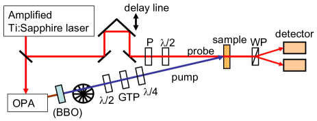
Figure 2: The experimental setup geometry. BBO was used for frequency doubling of the pump pulse, if necessary. WP: Wollaston prism, GTP: Glan–Taylor prism, P: polarizer, $\lambda/2$: half-wave plate, $\lambda/4$: quarter-wave plate.

We studied photoinduced spin precession in DyFeO₃ using a pump–probe magneto-optical technique, as shown in Fig. 2. DyFeO₃ single crystals were grown by the floating-zone method, and the orientation of the faces were determined by back-reflection x-ray Laue photographs.Tokunaga Faces with a width of few millimeters were mechanically polished. The sample thickness was 140 $\mu$m, except for a thickness dependent measurement. The sample was placed in a cryostat at 77 K with no external magnetic field. Optical pulses with a central wavelength of 790 nm, a duration of 150 fs, and a repetition rate of 1 kHz were emitted from an amplified Ti:sapphire laser. The beam was separated into two beams by a beamsplitter. One was employed as the probe beam, and the other was injected into an optical parametric amplifier (OPA), which converted the incident beam to signal and idler beams, in the wavelength ranges 1140–1580 nm and 1580–2570 nm, respectively. Furthermore, the signal and idler beams were frequency-doubled with a $\beta$-BaB₂O₄ (BBO) crystal if necessary. Then unwanted beams were cut by color filters. The ranges of the pump wavelength were 600–750 nm (second harmonic of the signal pulse), 850–1100 nm (second harmonic of the idler pulse), and 1140–1500 nm (the signal pulse).

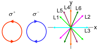
Figure 3: Pulse polarizations. Circularly polarized pulses are denoted $\sigma^{\pm}$. Linearly polarized pulses, denoted L1, L2, L3, L4, L5, and L6, were tilted at $-\pi/4,\pi/4,0,\pi/2,$ and $\mp\alpha$ from the $x$-axis, respectively, where $\tan\alpha=2$.

Figure 3 illustrates the circular and linear polarizations employed for the pump and probe pulses. Circularly polarized pulses are denoted as $\sigma^{\pm}$. Linearly polarized pulses, denoted L1, L2, L3, L4, L5, and L6, were tilted at $-\pi/4,\pi/4,0,\pi/2,$ and $\mp\alpha$ from the $x$-axis, respectively, where $\tan\alpha=2$.

The fluence of the pump pulse was varied from 15 to 130 mJ/cm², depending on the wavelength. The pump pulses were focused on the sample to spot sizes of 50–100 $\mu$m. The probe pulses were linearly polarized and had a pulse fluence of 1 mJ/cm². The probe beam was vertically incident on the surface of the sample, whereas the pump beam was incident at the angle of $7^{\circ}$. The transmitted probe pulse was divided into two orthogonally polarized pulses by a Wollaston prism, and each pulse was detected with a Si photodiode. The ratio of the signals from the detectors allowed us to determine the angle of the probe polarization.

III.2 Dependence of the polarization rotation on the pump pulse polarization

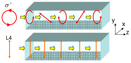
Figure 4: Polarizations of the propagating pulses in the medium with birefringence.

Figure 4 illustrates the polarization of the propagating pulses in the medium with birefringence. For the sake of simplicity, we will discuss the picture of the light propagation without taking the Faraday effect into account. Pulses with circular polarization or linear polarization nonparallel to the crystal axis are transformed, whereas pulses with linear polarization parallel to the crystal axis, corresponding to the normal modes of light in the media, are not. Thus, for the pulses with general linear polarization or pulses with circular polarization, the real and imaginary parts of $E_{x}E_{y}$, which are responsible for the terms in Eqs. (13)–(20) including $\sin 2\theta$, and $f_{xyz}$ and $g_{xyx}$, respectively, will oscillate in space along the pulse propagation direction, while they remain uniform only for pulses linearly polarized parallel to the crystalline axis. Therefore, the effective magnetic field and spin precession generated by IFE and ICME will be different at different positions in the sample.

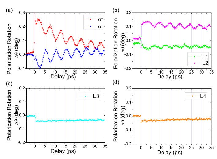
Figure 5: Oscillation of the probe polarization $\theta(t)$ as a function of the time delay between the pump and probe pulses. Six types of probe polarizations were used: (a) circular polarization $\sigma^{\pm}$, and linear polarizations tilted at (b) $\mp 45^{\circ}$, (c) $0^{\circ}$, and (d) $90^{\circ}$ with respect to the $x$-axis.

Figure 5 shows the polarization rotation of the probe pulse as a function of the delay time between the pump and probe pulses. The pump wavelength was 1050 nm, and the polarizations were $\sigma^{\pm}$, L1, L2, L3, and L4. The probe polarization was L4. When the pump polarizations were $\sigma^{\pm}$, L1, and L2, oscillation of the polarization rotation was observed. The frequency of the oscillation was 210 GHz at the temperature $T=77$ K, in agreement with previous infrared and Raman experiments.Balbashov ; Koshizuka ; White2 In Figs. 5(c) and (d), the pump pulses with polarizations L3 and L4 did not induce oscillation of the probe polarization. Polarizations $\sigma^{\pm}$, L1, and L2 had $E_{x}E_{y}$ components, but L3 and L4 did not, as shown in Fig. 4.

III.3 The influence of magnetization on the probe polarization

Modulation of the dielectric permittivity leads to oscillation of the probe polarization in the sample. The origin of the probe polarization change can be attributed to the Cotton–Mouton effect and the Faraday effect. The Cotton–Mouton effect is magnetic linear birefringence based on $\varepsilon_{xy}^{s}$, whereas the Faraday effect is magnetic circular birefringence based on $\varepsilon_{xy}^{a}$.

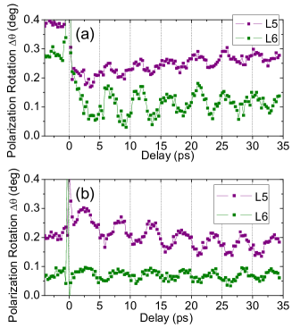
Figure 6: Time-resolved pump-induced probe polarization $\theta(t)$. The pump polarization was circular, and the graph shows the shift of the probe polarization when changing the pump polarization from $\sigma^{+}$ to $\sigma^{-}$. The pump wavelengths were (a) 750 nm and (b) 1050 nm, and the probe polarizations were L5 and L6.

In order to identify the effect giving rise to the polarization rotation as observed in Fig. 5, we set $\sigma^{\pm}$ for the pump polarization and L5 and L6 for the probe polarization. For L5 and L6, the Faraday effect leads to rotation of the probe polarization in the same direction for both probe polarizations, whereas the Cotton–Mouton effect leads to rotation in the opposite direction. Therefore, the dominance of the rotation of the probe polarization can be distinguished. Figure 6 shows that the polarization rotations of two probe pulses with polarizations L5 and L6 oscillated in the same direction. This indicates that the contribution of the Faraday effect is dominant and that of the Cotton–Mouton effect is negligible for the probe wavelength of 800 nm. This is consistent with the fact that IFE is dominant for the pump wavelength of 800 nm (see below).

III.4 Dependence of the polarization rotation on the pump wavelength

The oscillation of the probe polarization originates from spin precession. Therefore, the phase of the oscillation indicates the direction of an effective magnetic field induced by the pump beam. The dependence of the effective magnetic field and reorientation of magnetization on the pump wavelength gives information about the interaction of the light pulse and the magnetic medium.

An experiment was performed with four types of pump polarizations, $\sigma^{\pm}$, L1, and L2. The differences between the oscillations for $\sigma^{+}$ and $\sigma^{-}$ and between those for L1 and L2 were measured. Figure 7 (a) shows the initial phase $\xi$ of the oscillation of the probe polarization versus pump wavelength. The oscillation is described by $\theta(t)=A\sin(\omega t+\xi)$ at $t>0$, where $A$ is the amplitude, $\omega$ is the angular frequency, and $\xi$ is the initial phase. The initial phase was close to $0^{\circ}$ (or $\pm 180^{\circ}$), when the pump wavelength was 800 nm. This is consistent with Ref. Perroni, .

When the pump wavelength was between 1000 nm and 1100 nm, the initial phase was closer to $\pm 90^{\circ}$. When the pump wavelength was above 1200 nm, the initial phase was between $0^{\circ}$ and $90^{\circ}$. By comparing two samples with thicknesses of 140 $\mu$m and 170 $\mu$m, it was confirmed that the sample thickness does not affect the phase shift (data not shown). Figure 7 (b) represents the amplitude $A$ of the oscillation as a function of the pump wavelength. The amplitude $A$ is proportional to the pump fluence, thus justifying normalization of the amplitude by the fluence. Because of the transformation of the pulse polarization in the medium, the magnetic field differs at different positions. Therefore, the amplitude $A$ was not simply proportional to the magnitude of the generated magnetic field. However, when the pump wavelength was from 700 nm (${}^{6}A_{1}\rightarrow$ ${}^{4}T_{2}$) to 1000 nm (${}^{6}A_{1}\rightarrow$ ${}^{4}T_{1}$), the amplitude was larger than that of the other region in Fig. 7 (a). This result suggests that the photoinduced spin precession is related to the electron transition.

III.5 Pump–probe measurement in (100) and (010) oriented crystals

To determine all dielectric permittivities, we performed pump–probe measurements in (100) and (010) oriented crystals. The pump wavelength was 750 nm, and the crystal thickness in both cases was 100 $\mu$m. However, in contrast to the previous experiments,Kimel1 oscillation of the polarization of neither F- nor AF-modes was observed in either propagation direction.

III.6 The dependence of polarization rotation on temperature

It is well known that magnon frequencies in orthoferrites strongly depend on the temperature.Kimel1 ; Balbashov ; Koshizuka ; White2 We measured the temperature dependence of the spin precession properties in DyFeO₃. The frequencies of the oscillations for pump wavelengths of 750 nm and 1200 nm are shown in Fig. 8 (a), in comparison with previously reported spin precession.Balbashov Our data show excellent agreement with Refs. Kimel1, and Balbashov, , regardless of the pump wavelength. The frequency decreases with approaching the Morin point $T_{r}=37$ K because of magnon softening associated with the spin reorientation.Balbashov ; Koshizuka ; White2 The temperature dependence of the initial phase $\xi$ of the spin precession for pump wavelength of 750 nm is shown in Fig. 8 (b). The initial phase was close to 0^∘ or 180^∘ with a jump at $T$=150 K. It is worth to note that at this temperature the frequencies of F-mode and AF-mode become equal, that is $A(q_{3}-q_{1})=d^{2}-Aq_{1}$. Furthermore, the energies of two domain walls with the spin rotation in (010) and (001) planes become equal at this point, which leads to the reconstruction of domain walls.Zalesskii However, we were not able to find the relation between the properties described above and the initial phase shift.

IV DISCUSSION

IV.1 Landau–Lifshitz equations

According to the results of the previous section, the number of essential dielectric permittivity components can be reduced. First, we found that pump–probe measurement in (100) and (010) oriented crystals revealed that $\varepsilon_{zz}^{s}$, $\varepsilon_{xz}^{s}$, $\varepsilon_{yz}^{s}$, $\varepsilon_{xz}^{a}$, and $\varepsilon_{yz}^{a}$ were negligible. In addition, pump pulses with L3 and L4 polarizations did not trigger spin precession in the (001) oriented crystal in Fig. 5. Polarizations L3 and L4 had only electric field components $E_{x}$ and $E_{y}$, respectively. Therefore, the terms containing $\cos^{2}\theta$ and $\sin^{2}\theta$ in Eqs. (17), (18) and (20) were also negligible.

Moreover, it has been reported that $f_{xyz}M_{z}$ and $g_{xyx}L_{x}$ are of the same order of magnitude for orthoferrites.Woodfood1 In contrast to that, for the AF-mode the ratio of $m_{z}$ and $l_{x}$ is $|m_{z}/l_{x}|=|L_{x}/M_{z}|\simeq 100$. Thus, $f_{xyz}m_{z}\gg g_{xyx}l_{x}$, and one can ignore the term $g_{xyx}l_{x}$. In addition, Fig. 6 indicates that the observed oscillation of the polarization was dominated by the imaginary part of the dielectric permittivity $\varepsilon_{xy}^{a}=if_{xyz}(M_{z}+m_{z})+ig_{xyx}(L_{x}+l_{x})$. Because $f_{xyz}m_{z}\gg g_{xyx}l_{x}$, the phase of $m_{z}$ corresponds mostly to that of $\varepsilon_{xy}^{a}$ and that of the oscillation of the polarization.

These findings simplify the dielectric permittivity tensor. In Table 1, the tensor elements in the AF-mode column are proportional to $l_{x}$ and negligible, except for $\varepsilon_{xy}^{s}=(b_{xyxy}L_{x}+c_{xyzy}M_{z})l_{y}$ and $\varepsilon_{xy}^{a}=if_{xyz}m_{z}$. Here we suppose that a pulse is incident on a (001) oriented crystal. We can simplify the effective magnetic field and the dynamics of the magnetization induced by the circular polarization:

$$\textbf{{H}}^{{\rm eff,}\sigma^{\pm}}=\mp\frac{I_{0}\delta(t)f_{xyz}}{4}\hat{\mathbf{z}},$$ (21)

$$\textbf{{h}}^{{\rm eff,}\sigma^{\pm}}=0,$$ (22)

$$\Delta\textbf{{M}}^{\sigma^{\pm}}=0,$$ (23)

$$\Delta\textbf{{L}}^{\sigma^{\pm}}=\pm\frac{\gamma I_{0}f_{xyz}L_{x}}{4}\hat{\mathbf{y}}.$$ (24)

In the case of the linear polarization one in turn obtains:

$$\textbf{{H}}^{\rm eff,lin}=0,$$ (25)

$$\textbf{{h}}^{\rm eff,lin}=-\frac{I_{0}\delta(t)}{4}(2b_{xyxy}L_{x}+c_{xyzy}M_{z})\sin 2\theta\cdot\hat{\mathbf{y}},$$ (26)

$$\Delta\textbf{{M}}^{\rm lin}=\frac{\gamma I_{0}}{4}(2b_{xyxy}L_{x}^{2}+c_{xyzy}M_{z}L_{x})\sin 2\theta\cdot\hat{\mathbf{z}},$$ (27)

$$\Delta\textbf{{L}}^{\rm lin}=-\frac{\gamma I_{0}}{4}(2b_{xyxy}M_{z}L_{x}+c_{xyzy}M_{z}^{2})\sin 2\theta\cdot\hat{\mathbf{x}}.$$ (28)

The second terms are much smaller than the first ones in Eqs. (26), (27) and (28), respectively. As a result, IFE and ICME are induced by the contributions of $\varepsilon^{a}_{xy}$ and $\varepsilon^{s}_{xy}$, respectively.

Equation (24) indicates that the circular polarization causes the AFM component $l_{y}$ and rotation torque of the AF-mode. On the other hand, the FM component does not change in Eq. (23). As a result, IFE leads to oscillations proportional to $\sin\omega_{\rm AF}t$. On the other hand, Eqs. (27) and (28) indicate that linear polarization causes components $m_{z}$ and $l_{x}$. As shown in Fig. 1, $m_{z}$ and $l_{x}$ have the same phase, so ICME leads to oscillations proportional to $\cos\omega_{\rm AF}t$. Therefore, the initial phases of $m_{z}$ excited by IFE and ICME differ by 90^∘.

Because the phase of $m_{z}$ is nearly equal to that of the oscillation of the polarization, we can estimate the phase of spin precession from the result in Fig. 7. Since the polarization of the pump pulse is transformed by birefringence, the effective magnetic field and spin precession differ at different positions in the medium, as shown in Fig. 4. However, if one of IFE and ICME is dominant and the other is negligible, the time dependence of $m_{z}$ and the oscillation of the probe polarization are proportional to $\sin\omega_{\rm AF}t$ or $\cos\omega_{\rm AF}t$, respectively.

IV.2 Sigma model

Nonlinear sigma model is a convenient tool for the description of linear and especially non-linear spin dynamics of antiferromagnets, see Ref. Baryakhtar, for details. It is based on the dynamical equation for the vector $\bm{L}$ only that is of the second order in time derivatives, whereas the vector M is a slave variable so it can be expressed through the vector $\bm{L}$ and its time derivative. Recently, two alternative scenarios of laser-induced excitations of spin oscillations in antiferromagnets have been discussed within the framework of this model. The so-called inertial mechanism has been proposed for canted antiferromagnets and has been realized experimentally for holmium orthoferrite.Kimel3 Within the sigma-model approach, the inertial mechanism is associated with an action of the laser-induced pulse of the magnetic field on the vector $\bm{L}$ as a pulse of force on the massive particle. In this mechanism, the laser pulse creates an initial value of the time derivative, $d\bm{L}/dt$, that in principle can lead to quite large deviations of the vector $\bm{L}$ after the action of the pulse. In the alternative mechanism, the time derivative of the effective magnetic field plays a role of the driving force, leading to an initial deviation of the vector $\bm{L}$ from its equilibrium direction. Galkin ; Satoh1 For this field-derivative mechanism, the amplitudes of spin deviations are expected to be smaller than for inertial mechanism, but can be realized for any antiferromagnet, even a purely compensated one. The latter mechanism has beed observed experimentally in AFM nickel oxide, where the Dzyaloshinskii-Moriya interaction is forbidden by symmetry. Satoh1 It is interesting to understand which mechanism is responsible for the spin oscillations observed in the present work.

The Lagrangian density of the sigma model can be written as follows:Baryakhtar

$$\mathcal{L}=\frac{1}{8\gamma^{2}AM_{0}^{2}}\left(\frac{\partial\textbf{{L}}}{\partial t}\right)^{2}+\frac{1}{4\gamma AM_{0}^{2}}\left(\textbf{{H}}\cdot\left(\frac{\partial\textbf{{L}}}{\partial t}\times\textbf{{L}}\right)\right)+\frac{1}{A}(\textbf{{H}}\cdot(\textbf{{L}}\times\textbf{{d}}))-\mathcal{W}_{a}(\textbf{{L}})\,,$$ (29)

where H is the effective magnetic field and $\mathcal{W}_{a}(\textbf{{L}})$ is the effective anisotropy energy that includes $L$-dependent terms from the Hamiltonian (4) and a contribution from the Dzyaloshinskii-Moriya interaction, see Eq. (31) below. The slave variable, magnetic moment M, can be easily expressed via vector L and its time derivative,

$$\textbf{{M}}=\frac{\textbf{{L}}\times\textbf{{d}}}{A}+\frac{\textbf{{H}}L^{2}-\textbf{{L}}\left(\textbf{{L}}\cdot\textbf{{H}}\right)}{AL^{2}}+\frac{1}{\gamma AL^{2}}\left(\frac{\partial\textbf{{L}}}{\partial t}\times\textbf{{L}}\right)\,,$$ (30)

where $L=|\textbf{{L}}|$. Within the sigma-model approximation, the length of the vector L should be treated as a constant, $L_{x}^{2}+L_{y}^{2}+L_{z}^{2}=\mathrm{const}\simeq(2M_{0})^{2}$. Thus, in the linear approximation $L_{x}\simeq 2M_{0}-(l_{y}^{2}+l_{z}^{2})/4M_{0}$ and the two components, $l_{y}$ and $l_{z}$ can be considered as independent variables. It is in line with our experimental observation that the component $l_{x}$ is completely negligible. The effective anisotropy energy can be taken in the form

$$\mathcal{W}_{a}(\textbf{{L}})=\frac{1}{2}\left(q_{3}-q_{1}\right)l_{z}^{2}+\frac{1}{2}\left(\frac{d^{2}}{A}-q_{1}\right)l^{2}_{y}\,,$$ (31)

where the additive constant is omitted. Free oscillations of the two components at $\textbf{{H}}=0$ correspond to two independent magnon modes (F- and AF-modes), described by the following equations

$$\frac{d^{2}l_{z}}{dt^{2}} + \omega^{2}_{\mathrm{F}}l_{z}=0,\,\textbf{{m}}=\hat{\mathbf{x}}\frac{d}{A}l_{z}+\hat{\mathbf{y}}\frac{1}{2\gamma AM_{0}}\frac{dl_{z}}{dt}\,,$$

$$\frac{d^{2}l_{y}}{dt^{2}} + \omega^{2}_{\mathrm{AF}}l_{y}=0,\,\textbf{{m}}=-\hat{\mathbf{z}}\frac{1}{2\gamma AM_{0}}\frac{dl_{y}}{dt}\,.$$ (32)

Now let us discuss the excitations of the modes by light pulses. The interaction of the spin system with the light is described by the Hamiltonian (10), that for the specific case of circularly or linearly polarized light reads as (11) or (12), respectively. Within the sigma-model approach, for different polarizations the interaction terms enter different parts of the Lagrangian (29): the circularly polarized light contributes to the effective field $\textbf{{H}}=\textbf{{H}}^{{\rm eff,}\sigma^{\pm}}$, whereas the effect of the linearly polarized light is described by the time-dependent contribution

$$\delta\mathcal{W}_{a}(\textbf{{L}},t)=\frac{1}{4}\mathcal{E}_{i}(t)\mathcal{E}_{j}^{*}(t)b_{ijkl}L_{k}L_{l},$$ (33)

to the effective anisotropy energy $\mathcal{W}_{a}(\textbf{{L}})$. Among all these contributions to the Lagrangian, we need to find terms linear on $l_{y}$ and $l_{z}$, which produce the “driving force”, i.e., lead to a non-zero right-hand side in the equations of motion (32).

The light-induced effective field is directed along $z$-axis, and it is easy to see that the term $(\textbf{{H}}\cdot(\textbf{{d}}\times\textbf{{L}}))$ gives no “driving force” contributions for both modes. The gyroscopic term with $d\textbf{{l}}/dt$ provides such a term for $y$-component of the vector l, proportional to $H^{{\rm eff,}\sigma^{\pm}}_{z}L_{x}(dl_{y}/dt)$, but not for its $z$-component. Thus, for the state of interest ($\textbf{{L}}=L_{x}\hat{\mathbf{x}}$ in the ground state), the IFE can excite the AF-mode only. In the discussion presented above, the only part proportional to $b_{xyxy}L_{x}l_{y}$ gives an essential contribution to $\delta\mathcal{W}_{a}(\textbf{{L}},t)$. Using these relations, one can find that all the terms do not affect the equation for $l_{z}$ (F-mode), whereas the equation for $l_{y}$ describing the AF-mode acquires nonzero right-hand side and reads as

$$\frac{d^{2}l_{y}}{dt^{2}}+\omega^{2}_{\mathrm{AF}}l_{y}=-2\gamma M_{0}\frac{dH_{z}^{{\rm eff,}\sigma^{\pm}}}{dt}+A(2\gamma M_{0})^{2}h_{y}^{{\rm lin}},$$ (34)

where $h_{y}^{{\rm lin}}=-\partial\delta\mathcal{W}_{a}(\textbf{{L}},t)/\partial l_{y}$ is the effective field. Then, after the delta function substitution $\mathcal{E}(t)\mathcal{E}^{*}(t)\to I_{0}\delta(t)$, we arrive at the following initial conditions for this equation

$$\left(l_{y}\right)_{t=0}=\pm\frac{\gamma M_{0}f_{xyz}I_{0}^{\sigma^{\pm}}}{2}\,,$$ (35)

$$\left(\frac{dl_{y}}{dt}\right)_{t=0}=-4\gamma^{2}AM_{0}^{3}b_{xyxy}I_{0}^{{\rm lin}}\sin 2\theta,$$ (36)

where $I_{0}^{\sigma^{\pm}}$ and $I_{0}^{{\rm lin}}$ determine independent action of circularly and linearly polarized light, respectively, with $I_{0}^{\sigma^{\pm}}$ and $I_{0}^{{\rm lin}}$ being the corresponding integrated pulse intensities. As one can see from the equation, within the sigma-model approach the effective magnetic field created by the IFE enters the equation through its time derivative only, whereas the inertial mechanism is caused solely by ICME. Thus the field-derivative mechanism of the action of IFE, discussed previously for compensated antiferromagnets, Galkin ; Satoh1 is responsible for the excitation of spin oscillations in the $\Gamma_{4}$-phase of dysprosium orthoferrite investigated here. We conclude that it is difficult to realize the inertial mechanism of the field pulse action in the majority of orthoferrites at high temperatures where the same $\Gamma_{4}$-phase is present. The inertial mechanism has been observed for a special phase of holmium orthoferrite where the vector L is not collinear with the symmetry axis. Kimel3 On the other hand, for the present experiment the ICME leads to inertial mechanism of the spin excitations.

After the action of the pulse, only free spin oscillations persist in the system. They are described by the solution

$$l_{y}^{\mathrm{free}}=a\cos(\omega_{\mathrm{AF}}t+\xi),$$ (37)

$$m_{z}^{\mathrm{free}}=a\frac{\sqrt{d^{2}-Aq_{1}}}{A}\sin(\omega_{\mathrm{AF}}t+\xi),$$ (38)

where the amplitude $a$ and the phase $\xi$ are determined by the initial conditions (36) as follows:

$$\tan\xi=\mp\frac{4AM_{0}b_{xyxy}I_{0}^{{\rm lin}}\sin 2\theta}{f_{xyz}I_{0}^{\sigma^{\pm}}\sqrt{d^{2}-Aq_{1}}},$$ (39)

$$a=\gamma M_{0}\sqrt{\frac{\left(f_{xyz}I_{0}^{\sigma^{\pm}}\right)^{2}}{4}+\frac{\left(2Ab_{xyxy}M_{0}I_{0}^{{\rm lin}}\sin 2\theta\right)^{2}}{d^{2}-Aq_{1}}}.$$ (40)

Finally, we arrive at the previous result: if one of the two mechanisms, IFE or ICME, is dominating, the the phase of the $m_{z}$ oscillations takes the values $\xi=0$, $\pi$ or $\xi=\pm\pi/2$, respectively. Thus, the observed time dependence of the Faraday rotation oscillations is proportional to $\sin\omega_{\mathrm{AF}}t$ or $\cos\omega_{\mathrm{AF}}t$ for the dominating role of IFE or ICME, respectively. If none of the mechanisms is truly dominating, then the observed phase should take an intermediate value given by Eq. (40).

It is worth to note that the condition for domination of a certain effect does not translate into a plain comparison of the effective constant values $f_{xyz}$ and $2M_{0}b_{xyxy}$ for IFE and ICME, respectively. The point is, the ICME contributes through the inertial mechanism that is much more effective than the field-derivative mechanism involved in the action of IFE. In our calculation, this leads to appearance of the large multiplier $A/\sqrt{d^{2}-Aq_{1}}=\gamma H_{\mathrm{ex}}/\omega_{\mathrm{AF}}$, where $\gamma H_{\mathrm{ex}}\approx 20$ THz, $H_{\mathrm{ex}}=2AM_{0}\simeq$ 600 T is the exchange field of orthoferrite, Wijn in the contribution of ICME, see Eq. (40). Therefore the domination of IFE, for the same value of the pulse fluence, needs at least 50 times higher value of the corresponding constant, and the ratio $f_{xyz}/2M_{0}b_{xyxy}$ is expected to be large enough for orthoferrites. Thus, the above analysis gives us a possibility to estimate the values of constants responsible for different inverse magneto-optical effects, IFE and ICME.

IV.3 Comparison between the theory and the experiment

In the previous discussion, based on the Landau-Lifshitz equations and the nonlinear sigma model, we came to the conclusion that the time dependence of $m_{z}$ induced via IFE and ICME is proportional to $\sin\omega_{\rm AF}t$ and $\cos\omega_{\rm AF}t$, respectively. The phase of the oscillation is constant and $m_{z}$ is proportional to either $\sin\omega_{\rm AF}t$ or $\cos\omega_{\rm AF}t$ in some region of the pump wavelength in Fig. 7 (a). When the pump pulse is in the visible region ($<$800 nm), the probe polarization and $m_{z}$ oscillate as $\sin\omega_{\rm AF}t$. This property is independent of temperature as shown in Fig. 8 (b). On the other hand, when the pump pulse is in the near-infrared region (1000–1100 nm), the probe polarization and $m_{z}$ oscillate as $\cos\omega_{\rm AF}t$. Thus, we can conclude that the visible and near-infrared light pulses dominantly induce spin precession via IFE and ICME, respectively.

A number of reasons can be given for why the dominant effect varies with pump wavelength. IFE is induced by a pulse whose wavelength is near the transition ${}^{6}A_{1}\rightarrow$ ${}^{4}T_{2}$ at 700 nm. On the other hand, ICME is induced by a pulse whose wavelength is near the transition ${}^{6}A_{1}\rightarrow$ ${}^{4}T_{1}$ at 1000 nm. In addition, the Faraday rotation angle increases with decreasing wavelength in DyFeO₃.Tabor1 ; Chetkin This tendency agrees with the result for the IFE.

V CONCLUSIONS

We have studied the dependence of photoinduced spin precession in DyFeO₃ on the wavelength and polarization of a pump pulse with a pump–probe magneto-optical technique. The polarization rotation of the probe pulse was dependent on the pump polarization. Pulses propagating along the $z$-axis with both circular and linear polarizations induced an effective magnetic field (IFE and ICME) and spin precession. The dominant component of the dielectric permittivity in both effects was $\varepsilon_{xy}$, and IFE and ICME were induced by its antisymmetric and symmetric parts $\varepsilon_{xy}^{a}$ and $\varepsilon_{xy}^{s}$, respectively.

The phase and amplitude of the spin precession were dependent on the pump wavelength in DyFeO₃. A difference in the pump wavelength changes the dominant effect, giving rise to the spin precession. A visible pulse (wavelength $<$800 nm) induced the IFE, and the oscillation of the probe polarization was proportional to $\sin\omega_{\rm AF}t$. On the other hand, a near-infrared pulse (wavelength of 1000–1100 nm) induced the ICME dominantly, and the oscillation was proportional to $\cos\omega_{\rm AF}t$. When the pump wavelength was near the electron transition ${}^{6}A_{1}\rightarrow$ ${}^{4}T_{2}$ at 700 nm and ${}^{6}A_{1}\rightarrow$ ${}^{4}T_{1}$ at 1000 nm, the amplitude of the oscillation was larger than that of the other region.

The ratio of the effective magnetic fields via IFE and ICME, $f_{xyz}/2M_{0}b_{xyxy}$, is expected to be large enough for orthoferrites. However, the ellipticity of spin precession with AF-mode is also so large. Therefore, even though linearly polarized light pulse induces so weaker magnetic field than circularly polarized one, ICME can give the same order contribution as IFE.

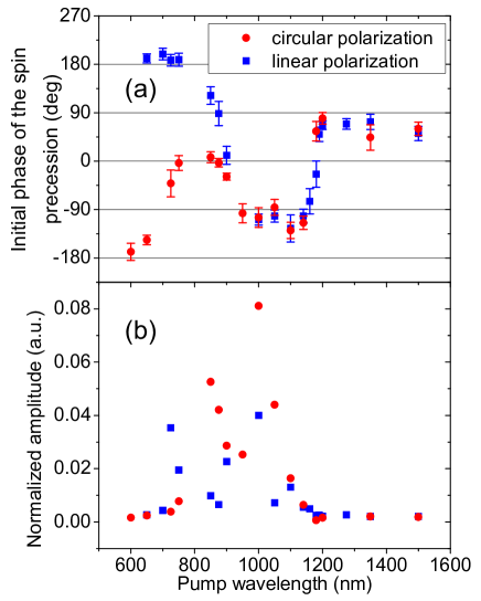
Figure 7: (a) Initial phase and (b) amplitude of the oscillation of the polarization as a function of the pump wavelength. The amplitude is normalized by the pump fluence.

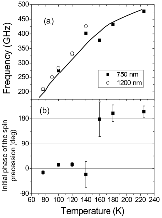
Figure 8: (a) Temperature dependence of the induced spin precession frequency. Pump wavelengths were 750 nm and 1200 nm. The solid line shows the magnon frequency taken from Ref. Balbashov, . (b) Temperature dependence of the initial spin precession phase for the pump wavelength of 750 nm.

References

- (1) E. Beaurepaire, J.-C. Merle, A. Daunois, and J.-Y. Bigot, Phys. Rev. Lett. 76, 4250 (1996).
- (2) J. Wang, C. Sun, J. Kono, A. Oiwa, H. Munekata, Ł. Cywiński, and L. J. Sham, Phys. Rev. Lett. 95, 167401 (2005).
- (3) B. Koopmans, M. van Kampen, J. T. Kohlhepp, and W. J. M. de Jonge, Phys. Rev. Lett. 85, 844 (2000).
- (4) G. Ju, A. Vertikov, A. V. Nurmikko, C. Canady, G. Xiao, R. F. C. Farrow, and A. Cebollada, Phys. Rev. B 57, R700 (1998).
- (5) F. Dalla Longa, J. T. Kohlhepp, W. J. M. de Jonge, and B. Koopmans, Phys. Rev. B 75, 224431 (2007).
- (6) A. V. Kimel, A. Kirilyuk, P. A. Usachev, R. V. Pisarev, A. M. Balbashov, and Th. Rasing, Nature (London) 435, 655 (2005).
- (7) T. Satoh, S.-J. Cho, R. Iida, T. Shimura, K. Kuroda, H. Ueda, Y. Ueda, B. A. Ivanov, F. Nori, and M. Fiebig, Phys. Rev. Lett. 105, 077402 (2010).
- (8) J. S. Dodge, A. B. Schumacher, J.-Y. Bigot, D. S. Chemla, N. Ingle, and M. R. Beasley, Phys. Rev. Lett. 83, 4650 (1999).
- (9) A. V. Kimel, A. Kirilyuk, A. Tsvetkov, R. V. Pisarev, and Th. Rasing, Nature 429, 850 (2004).
- (10) J. Zhao, A. V. Bragas, D. J. Lockwood, and R. Merlin, Phys. Rev. Lett. 93, 107203 (2004).
- (11) A. V. Kimel, B. A. Ivanov, R. V. Pisarev, P. A. Usachev, A. Kirilyuk, and Th. Rasing, Nature Phys. 5, 727 (2009).
- (12) J. Nishitani, K. Kozuki, T. Nagashima, and M. Hangyo, Appl. Phys. Lett. 96, 221906 (2010).
- (13) K. Yamaguchi, M. Nakajima, and T. Suemoto, Phys. Rev. Lett. 105, 237201 (2010).
- (14) T. Kampfrath, A. Sell, G. Klatt, A. Pashkin, S. Mährlein, T. Dekorsy, M. Wolf, M. Fiebig, A. Leitenstorfer, and R. Huber, Nat. Photon. 5, 31 (2011).
- (15) T. Higuchi, N. Kanda, H. Tamaru, and M. Kuwata-Gonokami, Phys. Rev. Lett. 106, 047401 (2011).
- (16) A. M. Kalashnikova, A. V. Kimel, R. V. Pisarev, V. N. Gridnev, A. Kirilyuk, and Th. Rasing, Phys. Rev. Lett. 99, 167205 (2007).
- (17) A. M. Kalashnikova, A. V. Kimel, R. V. Pisarev, V. N. Gridnev, P. A. Usachev, A. Kirilyuk, and Th. Rasing, Phys. Rev. B 78, 104301 (2008).
- (18) A. Kirilyuk, A. V. Kimel, and Th. Rasing, Rev. Mod. Phys. 82, 2731 (2010).
- (19) Y.-X. Yan, E. B. Gamble, and K. A. Nelson, J. Chem. Phys. 83, 5391 (1985).
- (20) R. Merlin, Solid State Commun. 102, 207 (1997).
- (21) A. V. Kimel, A. Kirilyuk, F. Hansteen, R. V. Pisarev, and Th. Rasing, J. Phys.: Condens. Matter 19, 043201 (2007).
- (22) H. P. J. Wijn, in Numerical Data and Functional Relationships, Landolt-Börnstein, New Series, Group III, Vol. 27F3 (Springer-Verlag GmbH, Berlin, 1994).
- (23) D. Treves, J. Appl. Phys. 36, 1033 (1965).
- (24) G. Gorodetsky, B. Sharon, and S. Shtrikman, J. Appl. Phys. 39, 1371 (1968).
- (25) R. L. White, J. Appl. Phys. 40, 1061 (1969).
- (26) V. G. Baryakhtar, M. V. Chetkin, B. A. Ivanov, and S. N. Gadetskii, Dynamics of Topological Magnetic Solitons: Experiment and Theory (Springer-Verlag, Berlin, 1994); V. G. Baryakhtar, B. A. Ivanov, and M. V. Chetkin, Sov. Phys. Usp. 28, 563 (1985).
- (27) Y. Tokunaga, S. Iguchi, T. Arima, and Y. Tokura, Phys. Rev. Lett. 101, 097205 (2008).
- (28) I. Dzyaloshinsky, J. Phys. Chem. Solids 4, 241 (1958).
- (29) T. Moriya, Phys. Rev. 120, 91 (1960).
- (30) G. F. Herrmann, J. Phys. Chem. Solids 24, 597 (1963).
- (31) A. M. Balbashov, A. A. Volkov, S. P. Lebedev, A. A. Mukhin, and A. S. Prokhorov, Sov. Phys. JETP 61, 573 (1985).
- (32) E. A. Turov, A. V. Kolchanov, V. V. Men’shenin, I. F. Mirsaev, V. V. Nikolaev, Phys. Usp. 41, 1191 (1998).
- (33) E. A. Turov, Physical Properties of Magnetically Ordered Crystals (Academic, New York, London, 1965).
- (34) G. Cinader, Phys. Rev. 155, 453 (1967).
- (35) N. Koshizuka and K. Hayashi, J. Phys. Soc. Jpn. 57, 4418 (1988).
- (36) F. J. Kahn, P. S. Pershan, and J. P. Remeika, Phys. Rev. 186, 891 (1969).
- (37) D. L. Wood, J. P. Remeika, and E. D. Kolb, J. Appl. Phys. 41, 5315 (1970).
- (38) W. J. Tabor and F. S. Chen, J. Appl. Phys. 40, 2760 (1969).
- (39) W. J. Tabor, A. W. Anderson, and L. G. Van Uitert, J. Appl. Phys. 41, 3018 (1970).
- (40) M. V. Chetkin, Ju. S. Didosjan, and A. I. Akhutkina, IEEE Trans. Magn. 7, 401 (1971).
- (41) G. A. Smolenskiĭ, R. V. Pisarev, and I. G. Siniĭ, Sov. Phys. Usp. 18, 410 (1975).
- (42) L. D. Landau and E. M. Lifshits, Course of Theoretical Physics, Vol. 8, Electrodynamics of Continuous Media (Pergamon, Oxford, 1984).
- (43) V. V. Eremenko, N. F. Kharchenko, Yu. G. Litvinenko, and V. M. Naumenko, Magneto-Optics and Spectroscopy of Antiferromagnets (Springer-Verlag, New York, 1992).
- (44) A. K. Zvezdin and V. A. Kotov, Modern Magnetooptics and Magnetooptical Materials (Taylor & Francis, New York, 1997).
- (45) C. A. Perroni and A. Liebsch, Phys. Rev. B 74, 134430 (2006).
- (46) R. M. White, R. J. Nemanich, and C. Herring, Phys. Rev. B 25, 1822 (1982).
- (47) A. V. Zalesskiĭ, A. M. Savvinov, I. S. Zheludev, and A. N. Ivashchenko, Sov. Phys. JETP 41, 723 (1976).
- (48) S. R. Woodford, A. Bringer, and S. Blügel, J. Appl. Phys. 101, 053912 (2007).
- (49) A. Yu. Galkin and B. A. Ivanov, JETP Lett. 88, 249 (2008).