Accuracy of core mass estimates in simulated observations of dust emission

Abstract

Aims. We study the reliability of the mass estimates obtained for molecular cloud cores using sub-millimetre and infrared dust emission.

Methods. We use magnetohydrodynamic simulations and radiative transfer to produce synthetic observations with spatial resolution and noise levels typical of Herschel surveys. We estimate dust colour temperatures using different pairs of intensities, calculate column densities with opacity at one wavelength, and compare the estimated masses with the true values. We compare these results to the case when all five Herschel wavelengths are available. We investigate the effects of spatial variations of dust properties and the influence of embedded heating sources.

Results. Wrong assumptions of dust opacity and its spectral index $\beta$ can cause significant systematic errors in mass estimates. These are mainly multiplicative and leave the slope of the mass spectrum intact, unless cores with very high optical depth are included. Temperature variations bias the colour temperature estimates and, in quiescent cores with optical depths higher than for normal stable cores, masses can be underestimated by up to one order of magnitude. When heated by internal radiation sources, the dust in the core centre becomes visible and the observations recover the true mass spectra.

Conclusions. The shape, although not the position, of the mass spectrum is reliable against observational errors and biases introduced in the analysis. This changes only if the cores have optical depths much higher than expected for basic hydrostatic equilibrium conditions. Observations underestimate the value of $\beta$ whenever there are temperature variations along the line of sight. A bias can also be observed when the true $\beta$ varies with wavelength. Internal heating sources produce an inverse correlation between colour temperature and $\beta$ that may be difficult to separate from any intrinsic $\beta(T)$ relation of the dust grains. This suggests caution when interpreting the observed mass spectra and the spectral indices.

1 Introduction

The initial conditions in cold molecular cloud cores determine many fundamental aspects of star formation: the stellar mass distribution, the star formation efficiencies, the main mode of clustered vs. isolated star formation, the evolution time scales etc. In particular, the stellar initial mass function (IMF) appears to be directly linked to the mass function of pre-stellar cores. In order to understand the star formation process, especially in its earliest phases, we must study the cold, pre-stellar cloud cores. In the cores many of the common molecular tracers have frozen onto dust grains. This makes it difficult to determine precise core properties from molecular line data and one has to resort to observations of the infrared and sub-millimeter dust emission. However, also the analysis of these data is not free from errors because temperature gradients and changes in dust emissivity may distort the column density estimates.

The core mass function (CMF) represents an intermediate stage between large scale cloud structure and turbulence and the final stellar population. Studies appear to confirm the similarity between the CMF and the IMF (Motte et al. motte98 (1998), motte01 (2001); Johnstone et al. (2000); Enoch et al. (2008); André et al. Andre2010 (2010)) but the observed mass spectra can be affected by several sources of uncertainty. The analysis may assume a constant dust temperature and, when several wavelengths are observed, the colour temperatures will be biased towards the highest actual dust temperatures along the line-of-sight. These systematic errors will have some effect also on the derived mass spectra. When protostars are formed within the cores, the internal heating will create even stronger temperature gradients that must be reflected in the mass estimates in a way that could be visible even in the details of the observed CMF. Also the used algorithms and their parameter values, or image acquisition techniques, can affect the derived CMF (e.g. Smith et al. smith08 (2008); Pineda et al. pineda09 (2009); Reid et al. reid2010 (2010)).

Several authors have investigated different aspects of star formation and the related observations with simulations (see e.g. Smith et al. (smith08 (2008)); Stamatellos et al. (stamatellos07 (2007), stamatellos10 (2010)); Urban et al. (urban09 (2010)); Shetty et al. (2009a , 2009b , shetty10 (2010))). In particular, Shetty et al. (2009b ) studied the effects of observational noise and temperature variations on the reliability of the derived dust properties. As expected, in the presence of temperature variations, the observationally derived dust spectral index $\beta$ underestimates the real spectral index of the dust grains. More surprisingly, the estimated colour temperatures are not only biased towards the warm regions but, in their two component models, were even higher than the physical temperature of either temperature component. The reliability of the spectral index determination is perhaps not as important for the mass estimation – although a wrong assumption of $\beta$ will automatically lead to wrong temperature estimates. However, the spectral index and its temperature dependence have received a lot of attention because they may provide additional information on the chemical composition, structure, and the size distribution of interstellar dust grains (e.g., Ossenkopf & Henning ossenkopf94 (1994); Krügel & Siebenmorgen Krugel1994 (1994); Mennella et al. Mennella1998 (1998); Mény et al. Meny2007 (2007); Compiègne et al. Compiegne2011 (2011)). The observations consistently show an inverse $T-\beta$ relation (e.g. Dupac Dupac2001 (2001), Dupac2003 (2003); Hill et al. Hill2006 (2006); Veneziani et al. Veneziani2010 (2010) and the initial Herschel results). The reliability of this relation is difficult to estimate because any noise present in the measurements also tends to produce a similar anticorrelation (see Shetty 2009a ). The absolute value of the dust opacity, $\kappa$, is also expected to vary because of changes in the abundance of different dust populations and changes in the grain size distribution. For the sub-millimeter observations, the changes should be strongest in dense and cold regions where the grains acquire ice mantles and may coagulate to form larger grains with much higher $\kappa$ values (e.g., Ossenkopf & Henning ossenkopf94 (1994), Krugel & Siebenmorgen Krugel1994 (1994), Stepnik et al. Stepnik2003 (2003)). The uncertainty of $\kappa$ affects directly any mass estimates. On the other hand, the absolute value of $\kappa$ is not easy to measure because it requires an independent column density estimate that is reliable over the same $A_{\rm V}$ range for which sub-millimetre observations exist. The total errors resulting from noise, temperature inhomogeneities, and dust variations are best estimated with modelling.

Magnetohydrodynamic (MHD) simulations are found to provide a good description for the general structure of interstellar clouds (Padoan et al. padoan2004 (2004, 2006)). When self-gravity is included, predictions can be made for the frequency and internal structure of dense cloud cores. Some of the objects that in continuum observations are categorized as cores may be transient while others will be held together by gravity and can potentially collapse forming stars. The models need to be compared with observations to see if the IMF can truly be explained as a direct consequence of the turbulent cascade (Padoan padoan95 (1995); Padoan & Nordlund padoan2002 (2002)). Nevertheless, the MHD runs already provide the best starting point for the realistic modelling of dust emission from dense clouds.

In this paper, we investigate the reliability of mass estimates by combining MHD simulations with radiative transfer modelling of dust emission. We start with some spherically symmetric (1D) models that help us to interpret the results of the more complex 3D clouds. We continue with low density contrast MHD models where we also test the consequences of spatially varying dust properties. We then present the first results from studies where we use cloud models that are defined with the help of hierarchical grids. With adaptive mesh refinement (AMR) one can follow the evolution of individual cores much further in the MHD calculations (see Collins et al. 2010a ) and, because of the stronger density and temperature variations, also the errors in the observationally derived core masses can be expected to be larger. Our main interest is not the shape of the CMF itself (as a result of the MHD modelling) but how the observational effects change the core mass estimates and to what extent these are visible in the observationally derived CMF. With the help of simulated observations, we can also draw some conclusions on the observability of dust spectral index variations.

The present study is relevant to many Galactic studies that are being conducted with the Planck (Tauber et al. Tauber2010 (2010)) and Herschel (Pilbratt et al. Pilbratt2010 (2010)) satellites. Herschel has already provided hundreds of new detections of both starless and protostellar cores (André et al. Andre2010 (2010); Bontemps et al. Bontemps2010 (2010); Könyves et al. Konyves2010 (2010); Molinari et al. Molinari2010 (2010); Ward-Thompson et al. WardThompson2010 (2010)) and detailed studies of these objects are now under way. In this context, it is crucial to know the uncertainties and the possible biases that might exist in the core and dust parameters that are derived from such sub-millimetre observations. The principal authors of this paper are also involved in the survey of Galactic cold cores that is being carried out with data from the Planck and Herschel satellites. The project will present an overview of the future galactic star formation areas by locating pre-stellar cores from the Planck all-sky survey and by following up a representative set of cores with higher resolution Herschel observations (see Juvela et al. Juvela2010 (2010)).

The methods used to create model clouds, to predict their sub-millimetre emission, and to analyse the resulting surface brightness maps are presented in Sect. 2. The results from the analysis are presented in Sect. 3, first for simple spherically symmetric cores (Sect. 3.1) and then for the cloud models based on MHD simulations (Sect. 3.2). Results of the estimation of dust spectral indices are presented in Sect. 3.3. We discuss the results in Sect. 4 before presenting our conclusions in Sect. 5.

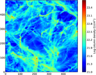
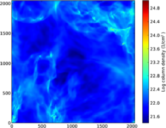
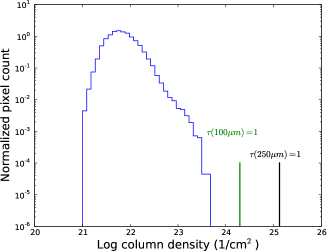
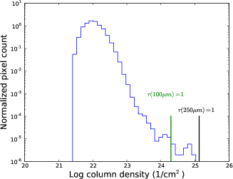
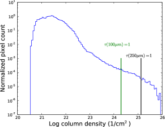
Figure 1: Column density maps (top row) and normalized column density distributions (bottom row) of Model I (left), Model II (middle) and Model III (right) in one viewing direction.

2 Methods

2.1 MHD simulations

We used three different cloud models to investigate the effects of different conditions in the dust clouds, mainly the opacity of the formed cores. The three models were all run in a similar fashion, with only the density and resolution changed. An isothermal equation of state was assumed in all MHD runs. All three models begin with the same non-gravitating turbulence simulation. A box of $1000^{3}$ zones with initially uniform density and magnetic field along the $\hat{z}$ axis was driven in a manner that maintained an rms sonic mach number of $\approx 9$. The initial plasma $\beta=8\pi P/B^{2}$, the ratio of thermal to magnetic pressure, is 22.2. The rms Alfvénic Mach number, the ratio of rms velocity to the Alfvén speed, is $\approx 2.8$. Stirring continues for several shock crossing times to statistically separate the turbulence from the initial conditions, at which time the simulation is re-gridded to three different resolutions, and gravity is switched on. Introduction of the gravity equation to the ideal MHD system imposes an additional physical scale on the system, and this is chosen differently for each of the three models.

Model I (Padoan & Nordlund padoan2010 (2010)) was continued with the Stagger code (Nordlund et al. nordlund96 (1996); Nordlund & Galsgaard nordlund97 (1997)) at a resolution of $500^{3}$. Stagger is a fixed resolution (unigrid) high order finite difference method. The code uses finite differences, with 6th order derivative operators, 5th order interpolation operators, and a 3rd order low memory Runge-Kutta time integration scheme.  Because of the staggered mesh, $\nabla\cdot B$ is conserved to machine precision. Box size and mean density are 6 pc and 450 $\rm{cm}^{-3}$, respectively.

Models II and III were continued with the MHD extension of the adaptive mesh refinement (AMR) code Enzo (Collins et al. 2010a ). It is a higher order Godunov method, using the patch solver of Li et al. (Li08 (2008)), the AMR technique of Balsara (Balsara01 (2001)), and constrains $\nabla\cdot B$ with the CT method of Gardiner & Stone (Gardiner05 (2005)). Model II was re-gridded to $128^{3}$, with size and density of 10 pc and $400\rm{cm}^{-3}$, and used 4 levels of refinement for an effective resolution of $2048^{3}$. This model was studied in detail in Collins et al. (2010b ). Model III used a root grid of $256^{3}$ and 4 levels of refinement, for an effective resolution of $4096^{3}$. It used the same box size as Model II, 10 pc, but a lower mean density of $144\rm{cm}^{-3}$. This model was allowed to run for a full free-fall time ($t_{ff}=\sqrt{3\pi/32G\rho}$) longer than Model II, which allows the cores to reach higher column densities, and thus opacities, while keeping a comparable number of cores.

The column density maps of the models are presented in Fig. 1. The figure shows also the distributions of the column density values in the models. Going from Model I to Model III, the peak column density increases more than two orders of magnitude, from $\sim 10^{23.5}$ to almost $10^{26}$ H cm^-2. In Model II, when observed with the highest resolution (distance=100pc, 37” beam), $\tau$(100 $\mu$m)=1.0 is reached only in one core, within an area smaller than the beam. In Model III the peak value is $\tau$(100 $\mu$m)$\sim$5 and $\tau$(100 $\mu$m)=1 is found in several cores, still limited to the size of a single beam (0.01% of all pixels in the full map). Therefore, even in Model III and even at 100 $\mu$m, the mean optical depth of the ’cores’ is always $\sim$1 or less.

The model of super Alfvénic turbulence has been compared to observations by a number of authors. Padoan et al. (Padoan99 (1999)) found that models with high Alfvén Mach number match column density and extinction statistics in the Perseus and IC 5146 clouds quite well, while models with stronger magnetic fields, thus lower Alfvén Mach number, do not. Crutcher et al. (Crutcher09 (2009)) measured the change in mass to flux from the envelope around a core to the core itself, and found the ratio, $\mathcal{R}$, to be inconsistent with the strong magnetic field prediction. Lunttila et al. (Lunttila08 (2008)) found similar values for $\mathcal{R}$ from a model similar to the turbulent initial conditions for all 3 models presented here. Collins et al. (2010b ) find excellent agreement between the data in Model II and Zeeman splitting measurements and mass distributions of dense cores in a number of different clouds.

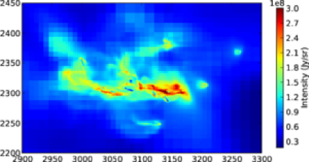
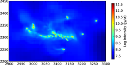
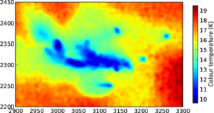
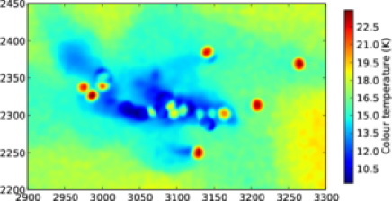
Figure 2: Closeups of the 250 $\mu$m intensity (top row) and colour temperature (bottom row) maps of Model III. The maps are shown before the addition of the internal radiation sources (left frames) and with the sources (right frames). The colour temperature was calculated from the ratio of 250 $\mu$m and 500 $\mu$m surface brightness.

2.2 Radiative transfer calculations

The MHD calculations provide the density distributions for our modelling. The clouds are illuminated externally by the interstellar radiation field (ISRF) (Mathis et al. Mathis83 (1983)) and, for the main part, the dust is assumed to have the average properties found in the Milky Way (Draine Draine2003 (2003)) with a gas-to-dust ratio of 124 and $R_{\rm V}$=3.1. Radiative transfer (RT) calculations are used to solve the dust temperature for each cell in the model and are independent from the gas temperature assumed in the MHD runs. The same RT program is used to calculate the emerging intensity by integrating the radiative transfer equation and without resorting to the assumption of optically thin emission.

The radiative transfer calculations of the unigrid model were carried out with our Monte Carlo radiative transfer program (Juvela & Padoan juvela03 (2003)). A separate radiative transfer program was used for the calculations on hierarchical grids. This second program is based on the unigrid code which has been modified to work with AMR grids and contains several associated improvements. The code will be described in detail elsewhere (Lunttila et al. in prep. ).

To investigate the effect of internal heating, black body radiation sources in the range of 0.3-120 solar luminosities were later added inside the gravitationally bound cores in Models II and III. The source temperatures were selected randomly between 200 K and 2000 K so that the distribution of log(T) was uniform. We assumed that a 0.1 M_☉ protostar has a luminosity of 10${}^{0.3}L_{\sun}$ and a 10 M_☉ protostar has a luminosity of 10${}^{2}L_{\sun}$. We applied linear interpolation on logarithmic scale for the other masses. The prescription is roughly consistent with the theoretical predictions of pre-main sequence evolution (see Wuchterl & Tscharnuter (wuchterl03 (2003), Fig. 3). The number of sources was 34 in Model II and 105 in Model III. In Model II the mass of the protostar was assumed to be 20% of the mass of the gravitationally bound core and in Model III the corresponding percentage was 50%. The model is not entirely self-consistent but sufficiently realistic so that we can study the basic observational effects caused by internal heating.

The cells in which the sources are located (‘source cells’) are not optically thin and the re-radiated dust emission is important in determining the dust temperature of the surrounding areas. Very close to the source, the assumption of a constant temperature within the cell also fails because of purely geometric effects. For these reasons, in the case of Model III, we used subgrid models to describe the temperature distribution of the source cells. We ran for each source a spherically symmetric (1D) radiative transfer model that was discretised to 100 shells and had an opacity equal to the opacity of the cell in the AMR model. In addition to the central sources, we assumed the 1D models to be illuminated externally by the ISRF. This was done in spite of the fact that the central sources completely dominate the radiation field even in the outer parts of the 1D models. The dust temperature profiles of the 1D models were solved iteratively taking into account the effects of re-radiated dust emission. In the full AMR model, the dust temperatures outside the source cells are below $30$ K which justifies the omission of the coupling with the dust opacity emission that would enter the 1D models from the outside. The 1D calculations also ignore the effect of other nearby sources. However, the sources are always tens of voxels apart so that contribution of other sources is negligible compared to the source residing inside the cell.

The 3D radiative transfer calculations were completed including the background radiation (ISRF), the radiation of the internal sources, and the dust emission from the medium. The average radiation field is dominated by the ISRF. When internal heating sources are included, they dominate the radiation field but only in their immediate vicinity. The re-radiated emission is completely insignificant far from the sources but very close to the sources can induce a small temperature raise (typically less than 1K). For the source cells the emission was already calculated with the 1D models but had to be still solved for the other cells. Because of the high optical depths, the calculations required iterations so that the effect of the sources (and the hot dust near the sources) could be transported outwards. The possibility of iterating arbitrary branches of the grid hierarchy separately (e.g., doing first sub-iterations just for the grids containing the sources) makes it possible to reach convergence much faster than by iterating the full model (see Lunttila et al. in prep. ).

Once the dust temperatures were solved, we do line-of-sight integration of the radiative transfer equation to calculate surface brightness maps at the finest resolution of the AMR model. Thus the maps of Model II contain 2048$\times$2048 pixels that correspond to a linear physical scale of 0.00488 pc or 1007 AU. The maps of Model III have 4096$\times$4096 pixels and a resolution 0.00244 pc or 503.6 AU. Maps were calculated for three orthogonal directions of observation ($X$, $Y$, and $Z$). As the final step in the simulation of surface brightness maps, we added to the maps noise typical of current Herschel observations (see Table 1) and convolved the maps to the resolution of the Herschel instruments at the corresponding wavelengths. The procedure depends on the assumed distance of the model cloud which was set to either 100, 400 or 1000 pc.

Table 1: Noise levels used to simulate typical Herschel observations.

Wavelength ($\mu$m)	$\sigma$ (MJy/sr/beam)
100	8.1
160	3.7
250	1.20
350	0.85
500	0.35

Closeups of Model III 250 $\mu$m intensity maps (without noise and convolution) and colour temperature maps before and after adding the sources are shown in Fig. 2. In the original intensity maps of Model III there are some dark ’worms’ in the densest and coldest cores. These are analogous to infrared dark clouds (e.g. Henning et al. henning2010 (2010)) but, because of the high opacity, are at high resolution visible up to sub-millimetre wavelengths. However, convolution of the maps hides these features. At longer wavelengths (e.g. 500 $\mu$m) the relative emission of these cold regions increases and such sharp absorption lanes are no longer seen.

2.3 Mass estimation

We begin the analysis by presuming the observer has only two wavelenghts available (e.g., Schnee & Goodman schnee2005 (2005), Kramer et al. Kramer2003 (2003), and Mitchell et al. Mitchell2001 (2001)). We use different wavelength pairs to compare how the results depend on the used wavelengths. We also compare these results to the case when all five Herschel wavelenghts are available.

The masses were first estimated with just two wavelengths, convolving the data to the resolution of the longer wavelength map. The wavelengths used were either 100 $\mu$m and 350 $\mu$m or 250 $\mu$m and 500 $\mu$m. The calculations were mostly performed with the correct value of the spectral index $\beta$. The analysis assumes optically thin emission and a dust opacity law of the form $\kappa\sim\nu^{\beta}$ so that the observed intensity can be written

$$I_{\nu}=B_{\nu}(T_{\rm C})(1-e^{-\tau})\approx B_{\nu}(T_{\rm C})\tau=B_{\nu}(T_{\rm C})\kappa N\propto B_{\nu}(T_{\rm C})\nu^{\beta}.$$ (1)

In our dust model the spectral index is 2.12 between 100 $\mu$m and 350 $\mu$m and 2.09 between 250 $\mu$m and 500 $\mu$m. In the case of two wavelengths and a fixed value of spectral index the modified black body law gives the temperature without any ambiguity (e.g., from the relative weight given for observations at different wavelengths). The dust colour temperatures $T_{\rm C}$ were determined from the ratio of the surface brightness at two wavelengths from the following equation

$$\frac{I(\nu_{1})}{I_{(}\nu_{2})}=\frac{B_{\nu_{1}}(T_{\rm C})\nu_{1}^{\beta}}{B_{\nu_{2}}(T_{\rm C})\nu_{2}^{\beta}}.$$ (2)

We also compared the results with an analysis where the colour temperature is estimated by fitting the modified blackbody function $B_{\nu}(T_{\rm C})\nu^{\beta}$ to observations at all five Herschel wavelengths. In the fit the free parameters were the scaling of the absolute level of the SED curve and the colour temperature. The spectral index $\beta$ was set to a fixed value or included as another free parameter of the fit.

Because of the added noise, the colour temperature estimates become very uncertain in the regions of the lowest column density. As a technical precaution the temperature was set to a constant value below a certain surface brightness level. This does not affect any of the discussion below because the regions containing the cores are well above this threshold and for them the colour temperature was always calculated pixel by pixel.

Once the colour temperatures were obtained, the column densities were calculated from the formula

$$N=\frac{I_{\nu}}{B_{\nu}(T_{\rm C})\kappa}$$ (3)

using the longer observed wavelength map. The selection of the wavelength (shorter vs. longer) is important only so far as the noise levels of the maps at the two wavelengths are different. When $T_{\rm C}$ was estimated by fitting the model SED to observations at several wavelengths, the column density was calculated from the same formula with the observed intensity and the correct opacity at the wavelength 250 $\mu$m. The column density is often calculated using the best-fit value of intensity. However, for the cores there is not much difference between using the best-fit or observed $I_{\nu}$ because of good S/N. The difference between the fitted and observed value of $I_{\nu}$ is about 1% at the wavelength 250 $\mu$m. With the dust opacity $\kappa$ expressed as area per hydrogen atom, the column density $N$ is obtained in units $H/$cm². In the calculations we use the correct value of the dust opacity that is obtained directly from the dust model. Therefore, neither the employed $\beta$ nor the $\kappa$ values should bias the subsequent mass estimates. The (hydrogen) mass per map pixel is calculated by multiplying the column density with the physical size of the pixel and the mass of the hydrogen atom. The masses are calculated either for fixed regions around the known core positions or for the clumps found with the Clumpfind algorithm (see Sect. 2.4). In both cases, the masses are obtained by summing the pixels assigned to that object. In spite of the convolution, the original pixel sizes were used throughout the analysis.

We use the term ’observed’ to describe also quantities derived from observations (e.g. temperature, column density, mass, spectral index or mass spectrum), in contrast with the corresponding quantities that are obtained directly from the model clouds. We compare the observed mass spectra with the ‘true mass spectra’. In both cases the clumps are identical and are extracted from the observed column density maps. While the observed mass spectra are calculated with the column densities derived from the simulated surface brightness maps, the ‘true mass spectra’ are derived using column densities that are read directly from the cloud model. Therefore, it is the ‘real’ mass spectrum only in the sense of not containing errors related to the derivation of column density from observations (‘observational errors’).

We compare the mass spectra with respect to their location on the mass axis and their general shape. To assist the visual inspection we use the slope of a least squares line fitted to a linear part as a numerical indicator of the shape. In some cases the result from the fit is not very reliable because of the absence of a clear linear part and the dependence on the mass range fitted.

2.4 Defining and finding cores

We use the CUPID implementation of the automatic clump finding method Clumpfind (Williams et al. williams94 (1994)) to locate cores in 2D column density maps in a similar manner as observers do. Because the number of pixels in our maps is larger than the resolution we have to scale the rms noise level of the background subtracted maps before using Clumpfind. We adopt the terminology where clump refers to larger structures and core to the densest condensations of the clumps (e.g. Stamatellos et al. stamatellos07 (2007)).

There has been some debate about the usability of Clumpfind in defining the shape of the CMF (see Smith et al. smith08 (2008); Goodman et al. goodman09 (2009) and Pineda et al. pineda09 (2009)). However, our main goal is not to study the absolute shape of the CMF but rather to examine the biases resulting from the way observations are usually analysed. Clumpfind also appears to find the densest cores in our 2D position–position data rather reliably with the right parameter values. However, parameter values must be determined independently for each case. Otherwise Clumpfind can easily start picking up sparse filaments as clumps in our high resolution and confusion-limited data. A problem with Clumpfind is that small changes in the parameter values can change the size and shape of the clumps significantly, especially when clumps become combined or separated.

The observed 2D clumps do not necessarily represent true 3D structures in the clouds due to projection effects (see eg. Shetty et al. shetty10 (2010)). This could also change the shape of the observed mass spectrum relative to the real spectrum that can be determined from the 3D data only. However, we do not have to take this effect into account because we are mostly comparing the observed and the true masses along the same full line-of-sight.

For the purpose of adding radiation sources into the gravitationally bound cores we have determined the positions by running the modified 3D Clumpfind over the 3D cloud model as in Padoan et al. (padoan2007 (2007)) and then selecting the sources for which $GE/(TE+KE+BE)>1$, that is the clumps in which the gravitational energy dominates over the sum of thermal, kinetic, and magnetic energy. In order to have a more objective definition of the core regions, and to eliminate the effects of Clumpfind algorithm, we also calculate the core masses within a fixed radius of these positions (projected to a map). With fixed radii we can also study how the mass estimates vary with the size of the region. This would of course not be possible in the analysis of normal observations but, in the case of models, provides a useful test where the effects of the clump selection are eliminated.

3 Results

3.1 Spherically symmetric reference models

To help the interpretation of the results of the 3D MHD models, we first study a series of spherically symmetric model clouds and examine the accuracy of the mass estimates in this simplified setting.

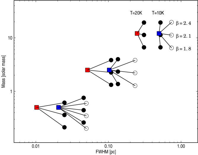
Figure 3: Observed properties of Bonnor-Ebert spheres. The solid squares denote the FWHM of the column density distribution and the true mass of the cores at $T_{\rm gas}=$10 K (blue symbols) or at 20 K (red symbols left of the 10 K points). The circles show the FWHM of the 350 $\mu$m surface brightness and the mass estimated from simulated observations at 100 $\mu$m and 350 $\mu$m. The cores are heated either by the full ISRF (open circles, shown for $T_{\rm gas}=$10 K only) or by the ISRF attenuated by A_V=4^m (filled circles). Masses are calculated with the correct spectral index, $\beta\sim 2.1$, and with one lower and one higher value.

3.1.1 Bonnor-Ebert cores

The density profiles of the spherically symmetric models follow the Bonnor-Ebert solution (Bonnor (1956)) with a stability parameter $\xi=6.5$ and a gas temperature of 10 K or 20 K. The cores are heated only by external radiation. Surface brightness maps are obtained from radiative transfer modelling and, as explained in Sect. 2.3 the core masses are calculated using observations at two wavelengths. The cores are assumed to be resolved so that the mass estimates are based on the derived column density profiles. We study three Bonnor-Ebert spheres that have masses of 0.5 $M_{\sun}$, 2.5 $M_{\sun}$, and 12.1 $M_{\sun}$. The corresponding average densities of the spheres are $2.2\times 10^{5}$, $8.8\times 10^{3}$, and $3.8\times 10^{2}$ H₂cm^-3.

Fig. 3 shows the results for a series of Bonnor-Ebert spheres comparing the real mass to the mass derived from 100 $\mu$m and 350 $\mu$m observations. The FWHM of the column density distribution is also compared to the FWHM of the 350 $\mu$m surface brightness. The open circles correspond to a case where the cores are illuminated by the full ISRF, the filled circles to a case where the ISRF is assumed to be attenuated by an external dust layer of $A_{\rm V}=4^{\rm m}$. The emission of this external layer is not included as would be the case if the analysis was carried out using background subtracted maps. The first scenario applies to isolated cores, the latter scenario would be more appropriate for cores inside molecular clouds.

When analysis is done with the correct spectral index, $\beta=$2.1, the mass estimates are mostly accurate to a few percent. Only for very compact clouds, represented here by the $0.5\,M_{\sun}$ core, the mass is clearly underestimated. For smaller Bonnor-Ebert spheres the column density and the temperature gradients between the centre and the surface are higher. The warm dust at the surface of the cores begins to dominate the signal, the colour temperature is higher than the average dust temperature, and the mass is underestimated. For the isolated core with $M=$0.5 $M_{\sun}$ and $T_{\rm gas}$=10 K the bias is $\sim$30%. If the incoming radiation is attenuated by $A_{\rm V}=4^{\rm m}$, the temperature gradients within the core decrease and the bias is reduced to a few percent. However, for $T_{\rm gas}$=20 K model the maximum error remains at $\sim$30%. At longer wavelengths the dependence on colour temperature is weaker and, for example, in typical Herschel observations these biases would not be a significant source of error. The uncertainty resulting from the unknown value of $\beta$ should be insensitive to the cloud properties. According to Fig. 3 the $\pm$0.3 uncertainty of the spectral index translates to a $\sim$30% error in the mass, almost irrespectively of the mass of the BE core. The mass estimate depends, of course, directly on the assumed dust opacity that in the case of real observations has a similar or even larger uncertainty.

Because of the cold centre of the cores, the intensity profiles are flat compared to the column density and the FWHM of the 350 $\mu$m intensity is higher than the FWHM of the column density. The difference is largest for the most compact clouds where, in fact, strong limb brightening is already seen at 100 $\mu$m.

3.1.2 High opacity cores

The previous tests showed that mass estimates are quite reliable for Bonnor-Ebert type cores. However, the errors should increase as the optical depth increases. The Bonnor-Ebert spheres represent a special case where the external pressure and gravity are balanced by the thermal pressure only. In the case of strong turbulent motions, rotation, or magnetic fields, stable cores may have higher opacity. For unstable cores, the optical depths will strongly increase during the collapse and, before the internal heating becomes important, observations might miss a larger fraction of the dust mass.

We investigated the possible effects purely from the standpoint of radiative transfer. We started with a one solar mass Bonnor-Ebert sphere ($T_{\rm gas}$=10 K, $\xi$=6.5) and, by multiplying its density with different constant factors, produced a series of models of increasing optical depth. Synthetic observations at two wavelengths were again analysed. This time the cores were assumed to be unresolved and the mass estimates were derived using the fluxes in an aperture with the size equal to the diameter of the core. The results are shown in Fig. 4. The relevant parameter is the cloud opacity which, of course, is here directly proportional to the mass of the core.

In Fig. 4a, in accordance with Fig. 3, the bias for the original Bonnor-Ebert sphere is about one third when the 100 $\mu$m and 350 $\mu$m observations are used. The bias is almost eliminated by either resorting to longer wavelengths (250 $\mu$m and 500 $\mu$m) or by reducing the temperature gradients by attenuating the external radiation field. In Fig. 4, the attenuation corresponded to $A_{\rm V}=8^{\rm m}$. When the optical depth is increased by a factor of ten, the error is a factor of five for an isolated core ($A_{\rm V}=0^{\rm m}$) observed at 100 $\mu$m and 350 $\mu$m. For the longer wavelength pair, similar bias is found only for opacities three orders of magnitude higher. The longer wavelengths are less sensitive to temperature errors and, unless observations contain significantly more noise, tend to give more accurate results.

In Fig. 4b, we consider the effect of a constant background that follows a spectrum $B_{\nu}($T=17 K$)\times\nu^{2}$ and the level of which is defined by its intensity at 100 $\mu$m, $I_{\rm bg}$. The core masses are now estimated from background subtracted observations. When 100 $\mu$m is included the core becomes colder and the 100 $\mu$m surface brightness becomes lower than the surface brightness of the background, and the core disappears. For the combination of 250 $\mu$m and 500 $\mu$m, the background has no effect before the opacities are two orders of magnitude higher than those of the original Bonnor-Ebert sphere. After that point, the mass estimates again briefly increase (relative to the real mass) before the absorption of the background again exceeds the emission.

In the analysis of 3D MHD runs, background subtraction will not be used. In that case, according to Fig. 4a, a factor of two errors in the mass estimates are not expected before the optical depths exceed the optical depth of the one solar mass Bonnor-Ebert sphere ($A_{\rm V}\sim 26^{\rm m}$ for $N(H)\sim 5\times 10^{22}$ cm^-2) by at least one order of magnitude.

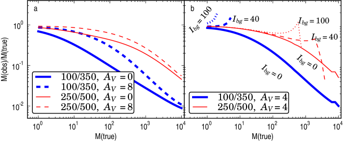
Figure 4: The ratio of observed mass and the real core mass for a series of models obtained by scaling the density of a one solar mass Bonnor-Ebert sphere. In frame $a$, the masses are determined with the 100 $\mu$m and 350 $\mu$m observations (thick lines) or the 250 $\mu$m and 500 $\mu$m observations (thin lines). The core is illuminated by the full ISRF (solid lines) or with a field that has been attenuated by $A_{\rm V}=8^{\rm m}$. Frame $b$ shows results for background subtracted observations after including a uniform background that at 100 $\mu$m has an intensity of 0, 40, or 100 MJy sr^-1.

3.2 MHD model clouds

3.2.1 Model I: Unigrid calculations and modified dust

As mentioned in Sect. 1, there are indications that in the dense and cold regions the dust sub-mm emissivity increases and emissivity index $\beta$ changes. Following the results of Ossenkopf & Henning (ossenkopf94 (1994)) we created a modified version of the employed dust model by changing the emissivity as shown in Fig. 5. The relative abundances of the normal and modified dust were set according to the density so that the abundance of the modified dust becomes significant only in the densest regions.

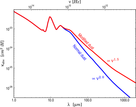
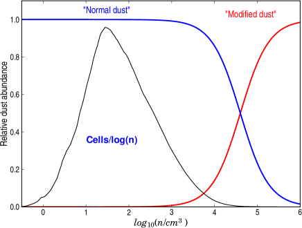
Figure 5: Dust opacities for the two dust models used (top) and their relative abundances as a function of density (bottom). The histogram shows the distribution of volume densities in Model I. The y-scale of the histogram is arbitrary.

The mass spectra obtained with the normal dust and with the mixture of normal dust and modified dust are shown in Fig. 6. The mass estimates were calculated with the 250 $\mu$m and 500 $\mu$m surface brightness maps and a distance of 400 pc. In the analysis, the emissivity index $\beta$ and the dust opacity $\kappa$ both corresponded to the actual values of the original dust model. Without the modified dust, the mass estimates were found to be almost completely unbiased. However, in the model containing also modified dust, the observed masses were strongly overestimated because in that case most of the dust found in the cores has a $\kappa$ value that is higher than what was assumed in the analysis of the observations. However, the difference is not as large as expected by the change in $\kappa$ alone which at 500 $\mu$m would be a factor of five. The mass errors increase when analysis is performed with $\beta=2$ that is larger than the actual value $\beta=1.5$ of the modified dust. The fact that masses are overestimated only by a factor of $\sim$3 (see Fig. 6) suggests that a large fraction of the observed intensity still comes from normal dust in regions surrounding the densest parts of the cores. The slope for the true mass spectrum (meaning one estimated with the true column densities) is $k=-1.2$ and for the observed mass spectrum $k=-1.3$, suggesting that the shape of the spectra does not change notably. The values correspond to the power law exponent -2.3 for $dN/dM$ similar to the values observed in real clouds (Enoch et al. (2008), Motte et al. motte98 (1998), Könyves et al. Konyves2010 (2010)).

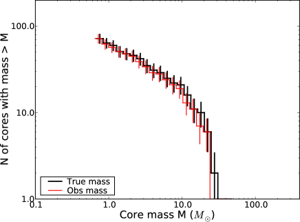
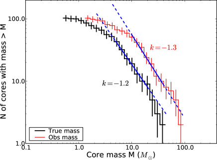
Figure 6: Model I: Cumulative mass spectra (with Clumpfind clumps) obtained with normal dust (top frame) and a modified dust model (bottom frame; see text). The analysis was carried out with observations at 250 $\mu$m and 500 $\mu$m and an assumed cloud distance of 400 pc. The slope (k) of the mass spectra is obtained by making a least squares fit to the linear part (marked with continuous line).

3.2.2 Model II: AMR model with cores of moderate opacity

Compared to Model I, Model II contains denser and more evolved cores and the resolution of the model is correspondingly much higher. The derived mass spectra of Model II are shown in Fig. 7. The analysis was done using the wavelengths 250 $\mu$m and 500 $\mu$m, the correct values of the $\kappa$ and $\beta$ parameters, and an assumed cloud distance of 100 pc. The clumps were searched with Clumpfind using three different parameter values as scaling factors for the rms noise (the uppermost frames in Fig. 7). For comparison, the masses were also calculated inside fixed radius regions around each projected centre position of the gravitationally bound cores (see Sect. 2.4). Three different radii were used: 30, 20, or 10 pixels (the third row of frames in Fig. 7).

The cumulative histogram plots of Fig. 7 compare the observed mass spectra with the ‘true mass spectra’. In both cases the clumps are identical and are extracted from the observed column density maps. With the Clumpfind clumps, the true and the observed mass spectra are almost indistinguishable, independently of the Clumpfind parameters and thus the number and spatial extent of the cores. Also the mass spectra obtained with regions of a 30 pixel radius show a close similarity and only at the highest densities the observed clump masses are somewhat underestimated. However, if we look at masses within 20 or 10 pixel radii, the masses are clearly underestimated in the high mass end. With 10 pixel radius the high mass end of true mass spectrum develops a hump that also deviates from the typical power law shape of mass spectra.

The mass spectra obtained with Clumpfind clumps (Fig. 7, row 2, middle frame) do not have a proper linear part. By fitting a slightly different mass interval the slopes can vary at least between values $k$ = -1.9 and -2.7. The slopes for the observed and true mass spectra obtained using clumps with a fixed 20 pixel radius (Fig. 7, row 4, middle frame) are $k$ = -4.2 and -2.5, respectively, indicating a clear change in the shape of the mass spectra. The mass spectra obtained with constant radius clumps do not adjust to the size of the clumps and because of this they depict more the column density than mass. Therefore these slopes cannot be directly compared to the CMF results reported from observations. The slopes for mass spectra with radius = 10 and 30 are given in the figure, but the values are highly dependent on the used mass interval.

In Fig. 7 the last row of figures compares directly the true and the observed masses within the circular regions around the positions of gravitationally bound cores. The effect that was seen in the mass spectra is even more apparent in these correlations. For a majority of the cores the masses are almost unbiased within all the three radii but in all cases there are several high density cores whose masses are severely underestimated. When the radius is decreased, the errors of the high density cores increase and the masses are systematically underestimated, sometimes by up to a factor of three.

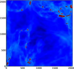
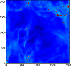
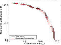
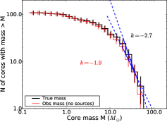
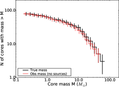
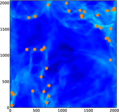
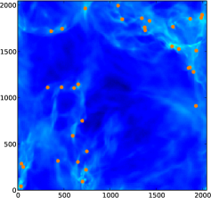
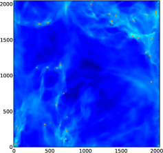
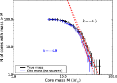
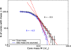
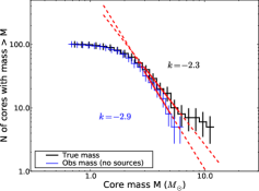
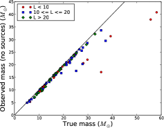
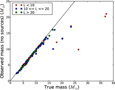
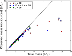
Figure 7: The comparison of Model II mass estimates obtained with different methods. The analysis was performed with surface brightness maps at 250 $\mu$m and 500 $\mu$m and an assumed cloud distance of 100 pc. Rows 1–2: The clump maps and mass spectra obtained with three different scaling factors for the rms noise. In the map the discovered clumps are drawn in red. The mass spectra are plotted using both the observed masses derived from the simulated observations (red line) and the true masses (but identical clumps) obtained from the cloud model. Rows 3–4: The results of similar analysis using areas within a fixed radius around the positions of gravitationally bound cores. The radius was 30 (leftmost frames), 20, or 10 pixels. The observed mass spectra is drawn with blue line in the electronic article in order to make a difference between the mass spectra obtained with Clumpfind clumps. Row 5: Relations of observed mass vs. true mass for the fixed radius environments. $L$ denotes the luminosity of the sources that are later added in the cores and is related to the mass of the original 3D clump. Here it acts only as an identifier for the masses of the cores. The clump areas are shown in only one direction, but in the mass spectra and observed mass vs. true mass plots clumps in all three directions are included. The slope (k) of some of the mass spectra is obtained by making a least squares fit to the linear part (marked with continuous line). Note that in middle frame on row 2 there is not a proper linear part. The slope values are very sensitive to the fitting interval.

We also calculated the colour temperatures using the wavelength pair 100 and 350 $\mu$m and the five wavelengths (100, 160, 250, 350, 500 $\mu$m). The relations of observed mass vs. true mass are shown in Fig. 8. Compared to the case with the wavelength pair 250 and 500 $\mu$m (Fig. 7, bottom row, middle frame), the observational bias is larger in both of these cases where shorter wavelengths were used. The case with wavelength pair 100 and 350 $\mu$m appears to have approximately the same mean value for the $M_{\rm true}/M_{\rm obs}$ relation as the case with five wavelengths, although with more scatter. Therefore smaller scatter does not imply smaller bias that is caused by the use of shorter wavelengths (100 $\mu$m and possibly 160 $\mu$m).

The observed and ’true’ spectral energy distributions (SEDs) of two cores (one with a small and one with a large mass error; see lower frame in Fig. 8) are shown in Fig. 9. With the ’true’ SED we mean the spectrum that corresponds to the true mean temperature of the dust grains, the true column density of the core, and the true $\beta$ of the dust. If a spectrum similar to the ’true’ SED was observed, we would get the correct mass estimate. The difference between the ’true’ and the observed SED is a measure of the temperature variations along the line-of-sight. At short wavelengths (less than $\sim$500$\mu$m) the intensity depends on the temperature nonlinearly which results in a difference between the colour temperature and the average grain temperature. As the colder dust emits less efficiently, the observed colour temperature is weighted towards the temperature in the warmest regions. This leads to overestimation of temperature and therefore to the underestimation of mass. As can be seen in Fig. 9, for the core with a small error in the mass the observed and ’true’ SEDs are very similar. In the case of the core with large observational mass bias (the high density core), the line-of-sight temperature variations are apparently stronger leading to a larger difference between the ’true’ spectrum and the warmer observed spectrum.

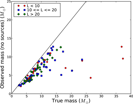
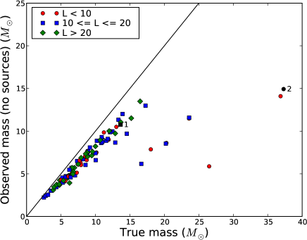
Figure 8: Model II: Relations of observed mass vs. true mass for the fixed radius environments with radius 20, distance of 100 pc and correct $\beta$. Colour temperature is calculated using wavelength pair 100 and 350 $\mu$m (top frame) and five wavelengths (100, 160, 250, 350, 500 $\mu$m) (bottom frame). The SED for the cores in bottom frame marked with black colour and numbers 1 and 2 are shown in Fig. 9.

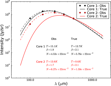
Figure 9: Model II: SEDs for the two cores (with radius = 20 pixels) that were marked with numbers 1 and 2 in Fig. 8. The “true” SEDs (see text) are drawn with continuous lines. The observed SEDs (dashed lines) are fits to five wavelengths 100, 160, 250, 350, and 500 $\mu$m and the corresponding mean intensities are marked with circles. Core 1 (with small observational mass bias) is marked with black and core 2 (with large observational mass bias) with red colour. For true SEDs: $T$ = true mean temperature of dust grains, $\beta$ = true spectral index = 2.1, $N$ = true mean column density for the core area. For observed SEDs: $T$ = temperature (given by fit), $\beta$ = spectral index (given by fit), $N$ = observed mean column density for the core area.

The effect of changing the value of $\beta$ that is used in the estimation of the colour temperatures is shown in Fig. 10. These mass spectra of Model II are obtained using wavelength pair 250 $\mu$m and 500 $\mu$m, assumed distance of 100 pc and regions of a fixed radius of 20 pixels. With a smaller value of $\beta$ the masses are underestimated more severely while the increase of $\beta$ by 0.2 units is enough to shift the observed mass spectrum roughly on top of the spectrum obtained with the correct column densities. However, the $\beta$ parameter does not affect the shape of the observed mass spectrum which remains steep (slope $k$ varies between -4.2 and -4.4 with all the used $\beta$ values) as the masses of the densest cores are still underestimated.

The mass hidden in the cold dust should become visible if the cores form protostars that start to heat up the cores from inside. To test this hypothesis, we added a radiation source to each gravitationally bound core as described in Sect. 2.2 and the analysis was repeated using the newly calculated surface brightness maps. The results are shown in Fig. 11 for one set of Clumpfind clumps and the 3D clumpfind cores using regions with the 20 pixel radius areas (giving slopes $k$ = -3.8 and -2.5 for observed and true mass spectrum, respectively). The Clumpfind parameters were the same as in the middle column frame of row 2 in Fig. 7. The addition of heating sources has not changed the situation for the Clumpfind spectra and, as before, the observed spectrum is consistent with the spectrum drawn with the true masses. In the case of fixed radius environments, the difference between observed and true masses is decreased. This is visible in the mass spectra but more clear when comparing directly the true and the observed masses of individual cores.

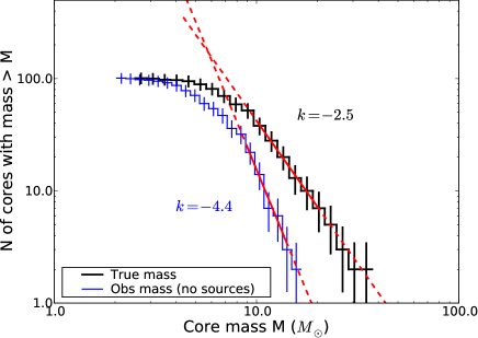
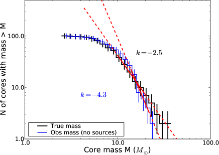
Figure 10: Model II: The effect of changing $\beta$ on mass spectra obtained with the wavelength pair 250 $\mu$m and 500 $\mu$m, assumed distance of 100 pc and environments of radius 20, $\beta=$1.8 (top) and 2.3 (bottom). The mass spectra obtained with correct $\beta\sim 2.1$ is shown in Fig. 7.

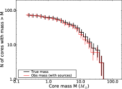
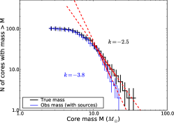
Figure 11: Model II with added sources using wavelength pair 250/500 $\mu$m, the correct value of $\beta$, and a distance of 100 pc. (Left) Mass spectra obtained with Clumpfind clumps. (Middle) The mass spectra obtained with environments of 20 pixel radius. (Right) The true vs. the observed masses within 10 pixel radii.

3.2.3 Model III: AMR model with cores of high opacity

The effective resolution of Model III is 4096³ cells. In our study, it represents the most evolved case and contains some cores with very high column density (Fig. 1).

For Model III the mass spectra with and without internal radiation sources are shown in Fig. 12. The spectra correspond to the objects found with Clumpfind. Unlike in Model II, without the internal radiation sources the core masses are significantly underestimated. The observed mass spectrum is much steeper than the spectrum obtained using the true masses. At the high mass end the shift in the spectrum corresponds to one order of magnitude in mass. The slopes for the observed and true mass spectra are $k$ = -1.9 and -1.4, respectively, indicating that there is a small change in the shape of the spectra. Once the radiation sources are turned on, the observed mass spectrum is almost completely rectified and a small difference remains only at the very highest masses.

The second row of frames in Fig. 12 compares the observed masses $m_{\rm obs}$ and the true masses $m_{\rm true}$ core by core using regions of 20 pixel radius. Without internal heating, the correct mass is recovered only for the smallest cores. When $m_{\rm true}$ reaches 40 $M_{\sun}$, the true mass is underestimated by a factor of ten although there is also significant scatter. When the internal sources are turned on, the bias disappears almost completely and is only $\sim$20% for the most massive cores. The cores are plotted with different symbols according to the luminosity that was assigned to the added sources. The luminosities depend monotonically on the mass of the gravitationally bound cores (see Sect. 2.2). However, the values plotted in Fig. 12 correspond to areas of the projected cloud and $m_{\rm true}$ often contains contribution from several 3D clumps that are close in the 2D projection. This explains why there is not a tight correlation between the source luminosity and $m_{\rm true}$. However, the luminosity assigned to the sources should still act as an identifier for the mass of the object at the centre of the areas examined. With this assumption one can say that, before the heating sources are added, the bias in the mass estimates increases with the object mass. This is clear below $\sim$10 $M_{\sun}$ but disappears at higher $m_{\rm true}$, presumably because these regions correspond to tight clusters of sources. When the radiation sources are included, the mass is underestimated mostly in the cores with the faintest sources. This may suggest that the heating power of our sources is generally only just enough to correct the mass estimates. The effects become clearer when we select a smaller radius (bottom frames in Fig. 12).

The size of the regions assigned to the cores appears to be important for the appearance of the mass spectra. Therefore, we tested the effect of different cloud distances in connection with the Clumpfind clumps of Model III. Because of the fixed beam sizes, a larger distance means lower linear resolution. In Fig. 13 are the results for cloud distances 400 pc and 1000 pc. The slopes for mass spectra are given in the figure, but the values are highly dependent on the used mass interval. The number of clumps identified with Clumpfind in the three cases, with distance of 100, 400, and 1000 pc, are 202, 161, and 144, respectively. The numbers include clumps counted towards all three directions. As the distance increases, the linear size of the identified clumps increases and some of the clumps are combined. As the average column density gets smaller, the observed masses approach the true masses. This means that the difference between the observed and the true mass spectrum decreases when resolution decreases. This could lead to very different CMFs between low resolution and high resolution studies of star formation.

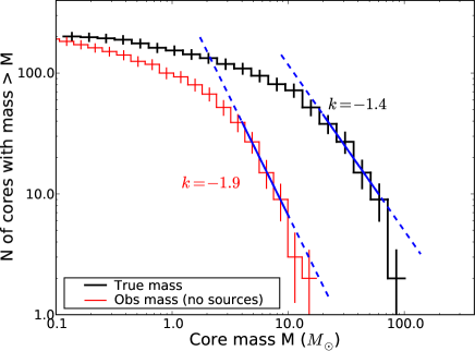
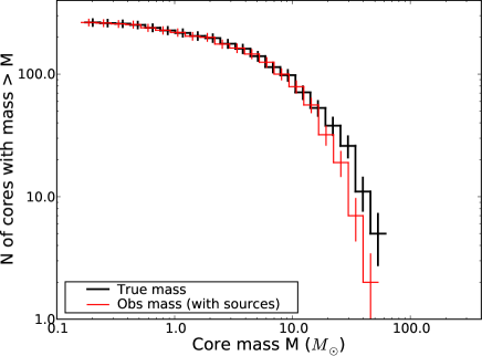
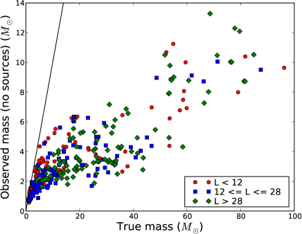
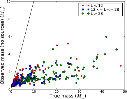
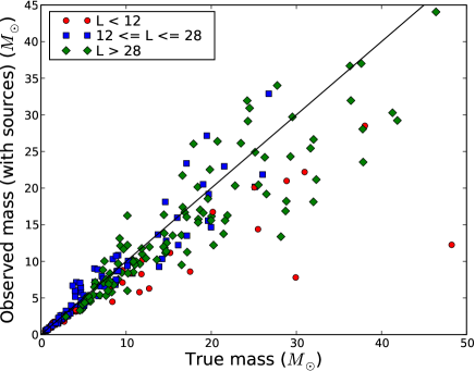
Figure 12: Model III: Mass estimates using wavelength pair 250/500 $\mu$m, the correct $\beta\sim$ 2.1, and a distance of 100 pc without (left column) and with (right column) internal heating sources. Rows from top: (1) Mass spectra obtained with Clumpfind clumps, (2) True vs. observed mass within regions of 20 pixel radius, (3) True vs. observed mass within regions of 10 pixel radius.

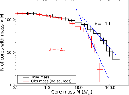
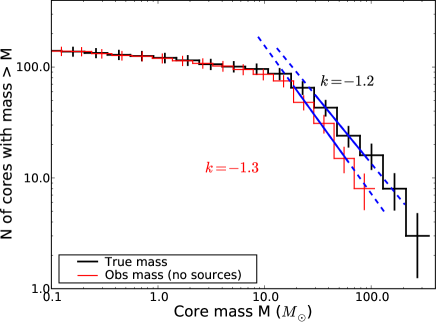
Figure 13: Model III: The effect of lower resolution (caused by longer distance) on the mass spectra obtained with Clumpfind clumps using wavelength pair 250/500 $\mu$m and the correct value of $\beta\sim$ 2.1. Distance to the cloud is 400 pc (top) and 1000 pc (bottom). Mass spectra obtained with a distance 100 pc (without sources) is shown in Fig. 12.

We investigated the effect of different wavelength pairs also in Model III and conclude that the masses obtained with the wavelength pair 100/350 $\mu$m compared to 250/500 $\mu$m are even more biased than in Model II.

3.3 Estimation of dust spectral indices

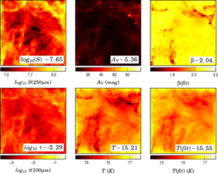
Figure 14: Results of the estimation of dust temperature and spectral index $\beta$ in Model II. The frames on the top row show the 250 $\mu$m surface brightness, the visual extinction, and the estimated spectral indices. On the bottom row are the logarithm of the 100 $\mu$m optical depth, the real mass averaged dust temperature along the line-of-sight, and the estimated colour temperature. The median values of the variables are given in the frames.

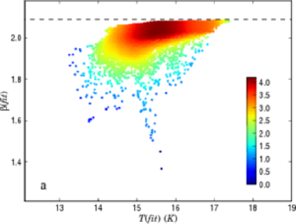
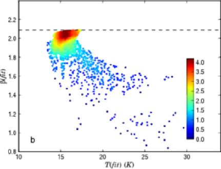
Figure 15: The correlation between the dust colour temperature and the spectral index as derived from the synthetic observations of Model II without internal sources (top frame) and with the internal heating sources (bottom frame). The colour scale indicates the logarithmic density of the ($T$, $\beta$) points and the dashed line the average spectral index in the dust model over the wavelength range used, 100 $\mu$m–500 $\mu$m.

The spectral index and its variations carry information on the intrinsic grain properties (see Sect. 1). Because of the strong anti-correlation between the temperature and the spectral index, accurate simultaneous determination of $T_{\rm dust}$ and $\beta$ is difficult in the presence of observational noise, as shown, e.g. by Shetty et al. ( 2009a ). We do not repeat those studies but concentrate on the importance of the line-of-sight temperature variations and the radiative transfer effects in our Model II. The dust colour temperature and the spectral index were obtained by a simultaneous fit of the simulated observations at 100 $\mu$m, 160 $\mu$m, 250 $\mu$m, 350 $\mu$m, and 500 $\mu$m. The analysis was carried out using data with maps convolved with a FWHM corresponding to 20 pixels and a pixel scale 0.049 pc. Noise was not added to the maps. After the convolution, the noise coming from Monte Carlo simulation is orders of magnitude below the noise level of typical observations. The effects discussed below arise from sources other than the noise.

Fig. 14 shows the results for Model II without internal sources. The estimated median temperature of 15.55 K is close to the real mass weighted average temperature of 15.21 K. However, the colour temperature is always higher than the dust temperature. The difference rises to $\sim$1 K in the most prominent filaments and reaches a peak value of $\sim$5 K towards the densest core. The spectral indices are correspondingly underestimated. The observed $\beta$ is close to the true value in diffuse regions, is too low by at least 0.1 units in the dense regions ($A_{\rm V}\sim 10$ or more), and is underestimated by up to 0.5 units towards the most opaque cores. This is seen more clearly in Fig.15 (top frame) which shows the correlation between $T_{\rm C}$ and $\beta$. For the main cloud of points, the spectral index decreases with decreasing temperature. The behaviour is opposite to the inverse $T-\beta$ relation that has been detected in interstellar clouds (e.g. Dupac et al. Dupac2003 (2003)). The result suggests that the intrinsic spectral index variations of dust could be much larger than what is directly observed towards quiescent clouds. The effect should be taken into account when seeking observational confirmation for the laboratory results that, after increasing towards lower temperatures, the sub-millimetre spectral index may again decrease as temperature falls below $\sim$10 K (Agladze et al. Agladze1996 (1996)).

We repeated the ($T_{\rm C},\beta$) estimation using only wavelengths 100 $\mu$m, 250 $\mu$m, and 350 $\mu$m. The results were qualitatively similar but the median colour temperature was lower, 14.92 K, and the median $\beta$ higher, 2.28. For most points, the spectral index was therefore higher than the intrinsic spectral index of the dust grains. In our dust model, the real $\beta$ between the wavelengths 100 $\mu$m and 350 $\mu$m is 2.12 but rises to $\beta$=2.21 between 250 $\mu$m and 350 $\mu$m. The reason for the high observed $\beta$ was traced back to this frequency dependence. In tests using a dust model with a constant $\beta$ over all wavelengths, the estimated $\beta$ remained below the real $\beta$ and approached that value only in diffuse regions. However, we could confirm with direct calculations, without the use of radiative transfer models, that when the spectral index varies with wavelength the fit of $B_{\nu}(T)\nu^{\beta}$ can result in $\beta$ values that are higher than the real beta anywhere in that wavelength range. The result suggests that such wavelength dependence can lead to significant error in the estimates of the spectral index and, therefore, in the dust temperature.

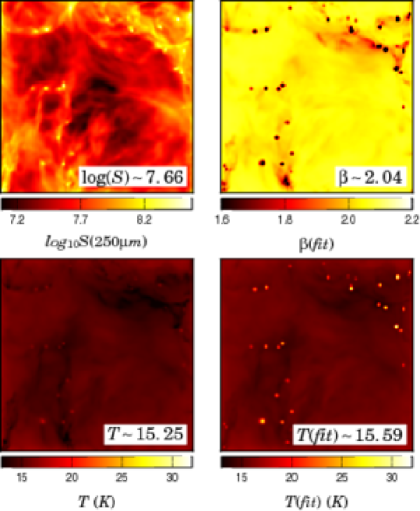
Figure 16: Results of the ($T_{\rm dust}$, $\beta$)- fits for Model II with internal sources. The frames on the top row show the 250 $\mu$m surface brightness and the derived spectral indices. The lower frames show the mass averaged line-of-sight dust temperature and the estimated colour temperature. The median value of the variables are quoted in the frames.

Fig. 16 and Fig.15 (bottom frame) show the results for Model II with the internal radiation sources. Because the sources have only a very local influence, the median value of $\beta$ is the same as before and the increase in the average temperature is small. However, because of the very strong temperature variations, the bias in the parameter values is now much larger towards the source regions. Furthermore, the internal heating increases the contribution of the densest cores which, at the full resolution of the cloud model, can reach optical depths $\tau(100\mu{\rm m})\sim$ 1. The opacity effects are no longer negligible while the colour temperature determination itself still assumes an optically thin emission. Because the spectral index is now underestimated towards cores that are warm, there is a strong anticorrelation between the temperature and spectral index (see Fig. 15 (bottom frame)) This effect is similar to the inverse relation observed in real clouds. This highlights the difficulty of separating the intrinsic dust properties from the effects produced not only by noise but also by radiative transfer effects. In particular, one must exercise caution when interpreting such observations when the samples include star forming clouds.

4 Discussion

The study showed that the shape of the mass spectrum is quite robust against errors arising from radiative transfer effects or spatial variations in dust properties. According to observations, the dust opacity varies from cloud to cloud. In particular, the difference between the diffuse and dense regions can be a factor of a few (e.g., Stepnik Stepnik2003 (2003)). Therefore, dust opacity remains a major factor of uncertainty in the estimation of cloud masses. We have excluded these errors by always using the correct dust opacity as obtained from the dust model. More generally, the mass estimates would of course be directly proportional to $\kappa^{-1}$. In our case the mass errors are caused by errors in the derived dust temperatures which, in turn, depend on the assumed spectral index or the procedure used to obtain $\beta$ from observations. For the masses of individual cores, the main errors result from the uncertain values of the dust opacity $\kappa$ and, to a lesser degree, the spectral index $\beta$. As long as these values are constant, the mass spectrum may be shifted but its shape is not much affected, unless the mass spectrum is based on optically thick central parts of the cores.

The errors resulting from radiative transfer effects were mostly smaller and even systematic and strong variations in the dust properties were not clearly visible in the shape of the derived mass spectra. Only if the cores have very high opacity (densest cores in our Model II and most cores of Model III), the effects resulting from the strong radial temperature variations become the main source of error, exceeding the uncertainty in $\kappa$.

It is often assumed that in dense and cold regions the dust sub-mm emissivity increases and emissivity index $\beta$ changes. If the change affected only the densest and presumably the most massive cores, the slope of the mass spectrum should become more shallow. Although we may have witnessed a very small change (see Fig. 6), even the drastic change implemented in the dust properties of Model I clearly had only a small effect on the shape of the mass spectrum. We also varied the threshold density at which the transition from normal dust to the higher emissivity dust takes place (Fig. 5). This did shift the mass spectrum along the mass axis but had no clear effect on the shape of the spectrum. It seems that, with a constant density threshold, the dust modification affects all cores almost equally. The denser cores have a higher abundance of modified dust but its contribution to the observed signal is small in relative terms because the modified dust resides in the coldest central parts of the cores and therefore radiates weakly. However, in denser cores the dust property variations could have a more important effect than in the more extended low density cores of Model I. In the AMR models we did not modify the dust. In future work this effect should be studied further.

The Clumpfind mass spectra obtained with Model II using the correct values of $\kappa$ and $\beta$ and wavelength pair 250 and 500  $\mu$m (Fig. 7) show that the mass estimates are very accurate. We compared also the Clumpfind results to masses within a constant radius of source positions. It is perhaps surprising that the differences between the observed and true masses that were very clear in the case of small radius regions are not seen with Clumpfind clumps. There are probably two reasons for this. Firstly, the Clumpfind clumps tend to be extended which is also visible in their larger masses. This is why Clumpfind is not so sensitive to the effects that are constrained to the densest cores of the clumps. Secondly, some of the compact cores for which the observed masses are the most severely underestimated are no longer found by the Clumpfind routine, depending on how strict criteria are used in finding clumps. The approximated size of the observed cores appears to be an important factor in the obtained mass spectra. As the core sizes increase the observed mass spectra approach the true mass spectra, as demonstrated by Fig. 7. The mass spectra obtained with Clumpfind clumps and environments of constant radius seem to give similar results, except with the densest cores with small radii. However, we could also limit the results of Clumpfind only to the densest cores. We conclude that when studying the details of mass spectra it is crucial to pay attention to the method of defining the clumps. The mass spectra obtained with constant radius cores cannot be directly compared to the CMF, as they depict more the column density than mass. However, the constant radius areas were a useful tool for studying the bias of mass estimates, independent of the uncertainties in the definition of the clumps.

We compared the mass estimates obtained using different wavelengths (wavelength pairs 250/500 $\mu$m, and 100/350 $\mu$m and five wavelengths (100, 160, 250, 350, 500 $\mu$m)) to calculate the colour temperature. The observational bias is larger if the shortest wavelengths are used compared to the case with wavelength pair 250 and 500 $\mu$m. Apparently the massive and dense cores contain significant amount of cold dust that is no longer seen at 100 $\mu$m. In our simulations only large grain particles are included. In real observations the intensity has a significant contribution from stochastically heated small particles at least up to wavelengths $\sim$100 $\mu$m. If no correction is made for this component, the masses derived from such observations will be even more strongly underestimated.

The SEDs in Fig. 9 show that for a high density core with large observational mass bias the observed SED differs clearly from the ’true’ SED obtained with true values of grain temperature, column density and $\beta$. Temperature variations on the line-of-sight lead to overestimation of temperature and through that to underestimation of mass.

The results in Fig. 13 for Model III showed that as the distance to the cloud increases and resolution decreases, the core sizes increase as smaller clumps are combined together and the mass estimates get more accurate. The mass estimates are worst for the densest regions. Therefore, by including more of the surrounding areas into the total mass, the mass will be larger but the relative error will be smaller.

In Model III with cores of high opacity the core masses are strongly underestimated even with correct values of $\kappa$ and $\beta$. This difference between Models II and III appears to be caused mainly by the difference in column density. In Model III the densest cores may have optical depths higher than for normal stable cores. Our tests showed that the errors in mass estimates become significant when the optical depths of the cores are one or several orders of magnitude higher than for normal Bonnor-Ebert spheres. This could be the case when strong turbulent motions, rotation, or magnetic fields are involved. Also for unstable cores, the optical depths will increase during the collapse. This means that before the internal heating becomes important, observations might underestimate the mass severely.

The estimates of the column density $N$ were based on the approximation of optically thin emission (see Eq. 1). In Model II, the maximum optical depth at 100 $\mu$m is about five and, even after the convolution with the beam (distance=100pc, 37” beam), can be up to one. In Model III, the optical depth at 100 $\mu$m can reach values of $\sim$5 even after convolution. Therefore, the approximation $\tau\ll 1$ is not valid everywhere in the cores. At least in a homogeneous medium, an increasing optical depth reduces short wavelength intensity relative to longer wavelengths. With the approximation of Eq. 1 this leads to lower colour temperature values. The effect counteracts the usual tendency to underestimate the column densities. This is illustrated in Fig. 17 for a case where observations consist of intensity measurements at 250 $\mu$m and 500 $\mu$m. The upper frame shows the situation for a homogeneous, 15 K slab as a function of the optical depth. Our use of the approximation $I_{\nu}=B_{\nu}(T_{\rm C})\nu^{\beta}$ results in the column density being overestimated. By fitting the observations with $I_{\nu}=B_{\nu}(T_{\rm C})(1-exp(-\kappa_{\nu}N))$, the correct value is recovered for all optical depths. The lower frame of Fig. 17 shows the situation when the model consists of two layers at different temperatures. A homogeneous slab at 7 K is placed behind another homogeneous layer at 15 K, the previous standing for 90% of the total optical depth that is shown on the horizontal axis. The line-of-sight temperature variation leads to significant underestimation of column density and the error is larger when we use the formula that is exact for homogeneous medium. This suggests that also in our 3D models the errors would have been larger if the analysis would have been completed without the assumption of optically thin emission. In Fig. 17 the difference between the two approaches is 20–30% when $\tau(250\,\mu{\rm m})$ is $\sim$1. However, the difference critically depends on the temperature structure of the cloud examined.

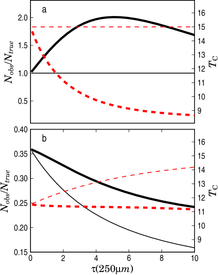
Figure 17: Comparison of colour temperature ($T_{\rm C}$, dashed lines) and the ratio of estimated and true column densities (solid lines) obtained from observations at 250$\mu$m and 500$\mu$m. The thick lines correspond to the optically thin approximation (cf. Eq. 1) and the thin lines to the values obtained by fitting $I_{\nu}=B_{\nu}(T_{\rm C})(1-exp(-\kappa N))$. Frame $a$ shows the results for a homogeneous model with a dust temperature of 15 K. In frame $b$ the model consists of two homogeneous slabs, with temperatures of 7 K and 15 K (see text for details). On the horizontal axis is the total opacity of the model cloud at 250 $\mu$m. The figure shows that while the exact formula gives correct values for a homogeneous model, it results in larger underestimation of column densities in case of the two layer model.

When there are internal heating sources that start to warm up the cores, the dust becomes easier to observe and the mass estimates get better. In Model II the sources do not change the mass spectrum notably, as it was nearly unbiased to begin with. The importance of the internal source varies, however, from core to core and the largest errors are still of the order of two. The effect of the radiation sources is very local so that a 20 pixel radius can encompass some very dense regions that remain unaffected by the central heating source. In Model III most of the strongly underestimated masses are corrected when internal sources start to make the densest cores visible. However, also in this model some of the core masses are still underestimated by a factor of 2–3. We have used internal sources that are strong enough to correct the mass estimates in most of the cores, but are also clearly visible in surface brightness maps. In future work it could be useful to study also weaker sources and how mass estimates depend on the characteristics of the sources and cores.

The spectral index $\beta$ and its temperature dependency can give information of the properties of interstellar dust grains. The observations (e.g. Dupac et al.Dupac2003 (2003)) show an inverse $T-\beta$ relation in interstellar clouds. However, it is difficult to estimate the reliability of this relation as noise can cause a similar anticorrelation (Shetty 2009a ). The results of Sect. 3.3 showed that temperature variations along the line-of-sight have a strong impact on the observed dust spectral index $\beta$. The value of $\beta$ was strongly underestimated in the direction of dense, inactive cores. This effect is opposite to the observed inverse $T-\beta$ relation. This could mean that in inactive clouds the spectral index variations are much larger than what is seen in the observations. However, in Model II the 100 $\mu$m optical depth approaches $\tau$=1 in some cores and this could also affect the derived values of $T$ and $\beta$. Shetty et al. (2009b ) studied the effects of noise and temperature variations on the estimation of dust properties. They found that estimated colour temperature values could be higher than the physical temperature of either of the two temperature components. We also found that the change of the spectral index as a function of wavelength can cause the value of the estimated spectral index to be higher than the true $\beta$ in our dust model. However, the effect was seen only when using three measurements in a wavelength range where the $\beta$ variations were strong. In SED fits employing five points spread over a wider wavelength range, the effect disappeared. This may indicate that such high $\beta$ values could appear only when three frequency points are fitted with a three parameter model that does not exactly fit the observations (i.e., assumes $\beta$ independent of wavelength). The effect depends on the actual shape of the observed spectrum which itself is affected not only by dust properties but also by the mixture of dust temperatures and other radiative transfer effects. Our results showed that protostellar sources in the cores can further increase the underestimation of the $\beta$ values. The cores are in this case warm and therefore this can produce a $\beta-T$ anticorrelation that is difficult to distinguish from any inherent $\beta(T)$ relation the dust grains may have. An error in $\beta$ causes an error in the estimated temperature and therefore also in masses.

5 Conclusions

We have examined the systematic errors in the analysis of sub-millimetre dust emission observations with the help of MHD model clouds and radiative transfer modelling. We have used different wavelength pairs to compare how the results depend on the used wavelengths. We have also compared these results to the case when all five Herschel wavelenghts are available. With three different models, we have determined the errors in the mass estimates of dense cores and how these are reflected in the shape of the core mass spectrum. Based on the results we draw the following conclusions:

• Because of line-of-sight temperature variations the core masses are usually underestimated. The effect varies strongly depending on the densities and possible internal heating of the cores.

• For normal cores, the largest uncertainties are still caused by the unknown values of the dust opacity $\kappa$ and, to a smaller extent, the spectral index $\beta$. In first approximation, both are multiplicative errors that leave the shape of the mass spectrum nearly unchanged. The opacity $\kappa$ is believed to vary by a factor of a few between diffuse and dense regions. According to our models, the error resulting from the bias in the colour temperatures is smaller.

• With the correct values of $\kappa$ and $\beta$, the mass estimates of normal cores in hydrostatic equilibrium are precise to some tens of percent. Although the systematic underestimation of mass is clear for individual dense cores and can shift the observed mass spectrum along the mass axis, the errors are not likely to be visible in the slope of the mass spectrum, unless the mass spectrum is based on optically thick central parts of the cores.

• If the cores have optical depths that are one or several orders of magnitude higher than expected for Bonnor-Ebert spheres, the errors in the mass estimates become significant. In our models, the real core masses were underestimated by up to a factor of ten. However, such dense cores are also unlikely to be detected even at sub-millimetre wavelengths, especially in regions of strong background emission.

• When observing cold dust, the temperature obtained with wavelength pair 250/500 $\mu$m gives more accurate mass estimates than the temperature obtained with a fit to 5 wavelengths, if shorter wavelengths ($\sim$100 $\mu$m) are included.

• The presence of internal heating sources can correct the mass estimates by making the dust in the core centres again visible. Even in the case of cores with very high opacity, the presence of a typical protostellar source reduces the bias in mass estimates to some tens of per cent.

• The observed dust spectral index $\beta$ was found to be affected strongly by the temperature variations along the line-of-sight (and within the detector beam). The $\beta$ value is strongly underestimated towards dense, quiescent cores. In SED fits using three wavelengths the spectral index was seen to be strongly overestimated because $\beta$ varied over the wavelength range in question. However, the effect was no longer seen in SED fits employing five frequency points.

• When the cores have internal radiation sources, the $\beta$ values are still strongly underestimated. Because the cores are in this case warm, this results in a $\beta-T$ anticorrelation that will be difficult to separate from any intrinsic $\beta(T)$ relation of the dust grains.

- (1) Agladze, N., Sievers, A., Jones, S., Burlitch, J., & Beckwith, S. 1996, ApJ, 462, 1026
- (2) André, P., Men’shchikov, A., Bontemps, S., et al. 2010, A&A, 518, L102
- (3) Balsara, D. S. 2001, Journal of Computational Physics, 174, 614
- Bonnor (1956) Bonnor, W.B. 1956, MNRAS, 116, 351
- (5) Bontemps, S., André, P., Könyves, V., et al. 2010, A&A, 518, L85
- (6) Collins, D. C., Xu, H., Norman, M. L., Li, H. & Li, S. 2010a, ApJS, 186, 308
- (7) Collins, D. C., et al. 2010b, accepted for publication to ApJ (http://adsabs.harvard.edu/abs/2010arXiv1008.2402C)
- (8) Compiègne, M., Verstraete, L., Jones, A., et al. 2011, A&A 525, 103
- (9) Crutcher, R., Hakobian, N., & Troland, T. 2009, ApJ, 692, 844
- (10) Draine, B.T. 2003, ARA&A 41, 241
- (11) Dupac, X., Giard, M., Bernard, J.-Ph., et al. 2001, ApJ, 553, 604
- (12) Dupac, X., Bernard, J.-P., Boudet, N., et al. 2003, A&A, 404, L11
- Enoch et al. (2008) Enoch, M. L., Evans, N. J., Sargent, A. I., et al. 2008, ApJ, 684, 1240
- (14) Gardiner, T. A. & Stone, J. M. 2005, Journal of Computational Physics, 205, 509
- (15) Goodman, A. A., Rosolowsky, E. W., Borkin, M. A., Foster, J. B., Halle, M., Kauffmann, J. & Pineda, J. E. 2009, Nature letters, 457, 63
- (16) Henning, Th., Linz, H., Krause, O., et al. 2010, A&A 518, L95
- (17) Hill, T., Thompson, M.A., Burton, M.G., et al. 2006, MNRAS, 368, 1223
- Johnstone et al. (2000) Johnstone, D., Wilson, C. D., Moriarty-Schieven, G., et al. 2000, ApJ, 545, 327
- (19) Juvela, M. & Padoan, P. 2003, A&A, 397, 201
- (20) Juvela, M., Ristorcelli, I., Montier, L., et al. 2010, A&A, 518, L93
- (21) Krügel, E. & Siebenmorgen, R., 1994, A&A, 288, 929
- (22) Könyves, V., André, P., Men’shchikov, et al. 2010, A&A, 518, L106
- (23) Kramer, C., Richer, J., Mookerjea, B., Alves, J., & Lada, C. 2003, A&A, 399, 1073
- (24) Li, S., Li, H. & Cen, R., 2008, ApJS, 174, 1
- (25) Lunttila, T., Padoan, P., Juvela, M., & Nordlund, Å. 2008, ApJ, 686, L91
- (26) Lunttila, T. et al., in preparation
- (27) Mathis, J.S., Mezger, P.G. & Panagia, N. 1983, A&A, 128, 212
- (28) Mennella, V., Brucato, J.R., Colangeli, L. et al. 1998, ApJ, 496, 1058
- (29) Mény, C., Gromov, V., Boudet, N., et al. 2007, A&A, 468, 171
- (30) Mitchell, G., Johnstone, D., Moriarty-Schieven, G., Fich, M., & Tothill, N. 2001, ApJ, 556, 215
- (31) Molinari, S., Swinyard, B., Bally, J., et al. 2010, A&A, 518, L100
- (32) Motte, F., Andre, P., & Neri, R. 1998, A&A, 336, 150
- (33) Motte, F., Andre, P., Ward-Thompson, D., et al. 2001, A&A, 372, 41
- (34) Nordlund, Å., Stein, R. F., & Galsgaard, K. 1996, in Lecture Notes in Computer Science, Vol. 1041, ed. J. Wazniewski, Proc. PARA95 Workshop, ed. J. Wazniewski, (New York : Springer), 450
- (35) Nordlund, Å. & Galsgaard, K. 1997, A 3D MHD Code for Parallel Computers (Tech. Rep., Astron. Obs., Copenhagen Univ.)
- (36) Ossenkopf, V., & Henning, Th. 1994, A&A, 291, 943
- (37) Padoan, P. 1995, MNRAS, 277, 377
- (38) Padoan, P., & Nordlund, Å. 2002, ApJ, 576, 870
- (39) Padoan, P., & Nordlund, Å. 2010, submitted
- (40) Padoan, P., Bally, J., Billawala, Y., Juvela, M., & Nordlund, Å. 1999, ApJ, 525, 318
- (41) Padoan, P., Jimenez, R., Juvela, M., & Nordlund, Å. 2002, ApJ, 604, L49
- (42) Padoan, P., Juvela, M., Kritsuk, A., & Norman, M. 2006, ApJ, 653, L125
- (43) Padoan, P., Nordlund, Å., Kritsuk, A., Norman, M., & Li, P. S. 2007, ApJ, 661, 972
- (44) Pilbratt, G., Riedinger, J., Passvogel, T., et al. 2010, A&A 518, L1
- (45) Pineda, J. E., Rosolowsky, E. W., & Goodman, A. A. 2009, ApJ, 699, L134
- (46) Reid., M., Wadsley, J., Petitclerc, N., & Sills, A. 2010, ApJ, 719, 561
- (47) Schnee, S., & Goodman, A. 2005, ApJ, 624, 254
- (48) Shetty, R., Kauffmann, J., Schnee, S., & Goodman, A. A. 2009a, ApJ, 696, 676
- (49) Shetty, R., Kauffmann, J., Schnee, S., Goodman, A. A., & Ercolano, B. 2009b, ApJ, 696, 2234
- (50) Shetty, R., Collins, D. C., Kauffmann, J., Goodman, A. A., Rosolowsky, E. W., & Norman, M. 2010, ApJ, 712, 1049
- (51) Smith, R. J., Clark, P. C., & Bonnell, I. A. 2008, Mon. Not. R. Astron. Soc., 391, 1091
- (52) Stamatellos, D., Whitworth, A. P., & Ward-Thompson, D. 2007, Mon. Not. R. Astron. Soc., 379, 1390
- (53) Stamatellos, D., Griffin, M. J., Kirk, J. M. et al. 2010, Mon. Not. R. Astron. Soc., 409, 12
- (54) Stepnik, B., Abergel, A., Bernard, J.-P., et al. 2003, A&A, 398, 551
- (55) Tauber, J., Mandolesi, N., Puget, J.-L., et al. 2010, A&A 520, 1
- (56) Urban, A., Martel, H., & Evans II, N. J. 2010, ApJ, 710, 1343
- (57) Veneziani, M., Ade, P.A.R., Bock, J.J., et al. 2010, ApJ, 713, 959
- (58) Ward-Thompson, D., Kirk, J.M., André, P., et al. 2010, A&A, 518, L92
- (59) Williams, J.P., de Geus, E. J., & Blitz, L. 1994, ApJ, 428, 693
- (60) Wuchterl, G., & Tscharnuter, W. M. 2003, A&A, 398, 1081