Numerical simulations of conversion to Alfvén waves in solar active regions

Abstract

We study the coupling of magneto-acoustic waves to Alvén waves using 2.5D numerical simulations. In our experiment, a fast magnetoacoustic wave of a given frequency and wavenumber is generated below the surface. The magnetic field in the domain is assumed homogeneous and inclined. The efficiency of the conversion to Alfvén waves near the layer of equal acoustic and Alfven speeds is measured calculating their energy flux. The particular amplitude and phase relations between the oscillations of magnetic field and velocity help us to demonstrate that the waves produced after the transformation and reaching upper atmosphere are indeed Alfvén waves. We find that the conversion from fast magneto-acoustic waves to Alfvén waves is particularly important for the inclination $\theta$ and azimuth $\phi$ angles of the magnetic field between 55 and 65 degrees, with the maximum shifted to larger inclinations for lower frequency waves. The maximum Alfvén flux transmitted to the upper atmosphere is about 2–3 times lower than the corresponding acoustic flux.

Conversion from fast-mode high-$\beta$ magneto-acoustic waves (analog of $p$ modes) to slow-mode waves in solar active regions is relatively well studied both from analytical theories and numerical simulations (e.g., [1, 2, 3, 4, 5, 6]), see [7] for a review. In a two-dimensional situation, the transformation from fast to slow magnetoacoustic modes is demonstrated to be particularly strong for a narrow range of the magnetic field inclinations around 20–30 degrees to the vertical. However, no generalized picture exists so far for conversion from magneto-acoustic to Alfvén waves in a three-dimensional situation. Studies of this conversion were initiated by Cally & Goossens [8], who found that the conversion is most efficient for preferred magnetic field inclinations between 30 and 40 degrees, and azimuth angles between 60 and 80 degrees, and that Alfvénic fluxes transmitted to the upper atmosphere can exceed acoustic fluxes in some cases. Newington & Cally [9] studied the conversion properties of low-frequency gravity waves, showing that large magnetic field inclinations can help transmitting an important amount of the Alfvénic energy flux to the upper atmosphere.

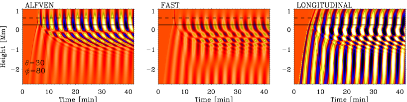
Figure 1: Time-height variations of the three projected velocity components corresponding to $\hat{\mathbf{e}}_{\rm perp}$ (Alfven wave, left), $\hat{\mathbf{e}}_{\rm tran}$ (fast wave, middle) and $\hat{\mathbf{e}}_{\rm long}$ (slow wave, right) for $\nu=5$ mHz in a simulation with $B$ inclined by $\theta=30^{\circ}$ and $\phi=80^{\circ}$. The solid line marks the position $c_{S}=v_{A}$, and the dashed line marks the cut-off layer $\nu=\nu_{c}\cos\theta$. The colour scaling is the same in all panels. The amplitudes are scaled with $\sqrt{\rho_{0}v_{A}}$ (first two panels) $\sqrt{\rho_{0}c_{S}}$ (last panel).

Motivated by these recent studies, here we attack the problem by means of 2.5D numerical simulations. The purpose of our study is to calculate the efficiency of the conversion from fast-mode high-$\beta$ magneto-acoustic waves to Alfvén and slow waves in the upper atmosphere for various frequencies and wavenumbers as a function of the field orientation. We limit our study to a plane parallel atmosphere permeated by a constant inclined magnetic field, to perform a meaningful comparison with the work of Cally & Goossens [8]. Numerical simulation will allow generalization to more realistic models in our future work.

We numerically solve the non-linear equations of ideal MHD assuming all vectors in three spatial directions and all derivatives in two directions (i.e. 2.5D approximation, see [10, 11]), though perturbations are kept small to approximate the linear regime. An acoustic wave of a given frequency and wave number is generated at $-5$ Mm below the solar surface in a standard model atmosphere permeated by a uniform inclined magnetic field. The top boundary of the simulation box is 1 Mm above the surface, and 0.8 Mm above the layer where the acoustic speed, $c_{S}$, and the Alfvén speed, $v_{A}$, are equal. We consider frequencies $\nu=3$ and 5 mHz and wave numbers $k_{X}=1.37$ Mm^-1 and $k_{Y}=0$. The simulation grid covers field inclinations $\theta$ from 0^∘ to 80^∘ and field azimuths $\phi$ from 0^∘ to 160^∘. The field strength is kept at $B=500$ G. To separate the Alfvén mode from the fast and slow magneto-acoustic modes in the magnetically dominated atmosphere we use velocity projections onto three characteristic directions:

$$\hat{\mathbf{e}}_{\rm long} = [\cos\phi\sin\theta,\,\sin\phi\sin\theta,\,\cos\theta];$$

$$\hat{\mathbf{e}}_{\rm perp} = [-\cos\phi\sin^{2}\theta\sin\phi,\,1-\sin^{2}\theta\sin^{2}\phi,\,-\cos\theta\sin\theta\sin\phi];$$ (1)

$$\hat{\mathbf{e}}_{\rm trans} = [-\cos\theta,\,0,\,\cos\phi\sin\theta].$$

To measure the efficiency of conversion to Alfvén waves near and above the $c_{S}=v_{A}$ equipartition layer, we calculate acoustic and magnetic energy fluxes, averaged over time:

$${\bf F_{ac}}=\langle p_{1}{\bf v}_{1}\rangle;\qquad{\bf F_{mag}}=\langle{\bf B_{1}}\times({\bf v}_{1}\times{\bf B_{0}})/\mu_{0}\rangle.$$ (2)

Figure 1 shows an example of the projected velocities in our calculations as a function of space and time. In this representation the larger inclination of the ridges mean lower propagation speeds and vice versa. Note, that by projecting the velocities, we are able to separate the modes only in the magnetically dominated atmosphere, i.e. above the solid line in Fig. 1. The figure shows how the incident fast mode wave propagates to the equipartition layer and then splits into several components. The Alfvén wave is produced by mode conversion above 0.2 Mm (left panel) and propagates upwards with the (rapid) Alfvén speed, confirmed by almost vertical inclination of the ridges. Conversely, the essentially magnetic fast-mode low-$\beta$ wave produced in the upper atmosphere (middle panel) is reflected, and its velocity variations in the upper layers vanish with height. The (acoustic) slow-mode low-$\beta$ wave escapes to the upper atmosphere tunnelling over the cut-off layer due to the field inclination of $\theta=30^{\circ}$. The amplitudes of the velocity variations of the Alfvén wave are comparable to those of the slow wave.

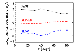
Figure 2: Left panel: Log₁₀ of the ratio $B_{1}$ to $V_{1}/\sqrt{\mu_{0}\rho_{0}}$ for projected velocities and magnetic field variations, averaged over all $\phi$, as a function of $\theta$. Black line: fast mode ($\hat{\mathbf{e}}_{\rm tran}$ projection); red line: Alfvén mode ($\hat{\mathbf{e}}_{\rm perp}$); blue line: slow mode ($\hat{\mathbf{e}}_{\rm long}$). Right panel: phase shift between the projected variations of $V_{1}$ and $B_{1}$, as a function of $\theta$ for selected $\phi$. Red lines: Alfvén mode; black lines: fast mode.

To confirm the Alfvén nature of the transformed waves, as revealed by the projection calculations, we checked the amplitude and phase relations for all three modes reaching the upper atmosphere. For the Alfvén mode the magnetic field $B_{1}$ and velocity variations $V_{1}$ should be in equipartition (i.e. $B_{1}=V_{1}/\sqrt{\mu_{0}\rho_{0}}$), and both magnitudes should oscillate in phase (see Priest [12]). Figure 2 presents the calculations of the amplitude ratio $B_{1}\sqrt{\mu_{0}\rho_{0}}/V_{1}$ and temporal phase shift between $B_{1}$ and $V_{1}$, where both velocity and magnetic field variations are projected in the corresponding characteristic direction for each mode (Eq. Numerical simulations of conversion to Alfvén waves in solar active regions). This calculation confirms that, indeed, for all magnetic field orientations $\theta$ and $\phi$, the amplitude ratio for the Alfvén mode ($\hat{\mathbf{e}}_{\rm perp}$ projection) is around one (left panel). This is clearly not the case for the slow and fast modes. For the fast mode, the amplitude ratio is two orders of magnitude larger, and for the slow mode, it is two orders of magnitude lower than one. For the Alfvén mode the phase shifts group around zero for all $\phi$, unlike the case of the fast mode (right panel). We did not calculate the phase shifts for the slow mode as the variations of the magnetic field are negligible. Thus, we conclude that the properties of the simulated Alfvén mode separated by the projection correspond to those expected for a classical Alfvén mode.

Figure 3: Examples of the height dependence of the magnetic (solid line) and acoustic (dashed line) vertical fluxes, defined by Eq. 2, for $\nu=5$ mHz and several $\theta$ and $\phi$. Solid vertical line marks the position $c_{S}=v_{A}$, dashed vertical line marks the cut-off layer $\nu=\nu_{c}\cos\theta$.

An example of the height variations of the acoustic and magnetic fluxes is given in Figure 3. The total vertical flux (dotted line) is conserved in the simulations except for the limitations caused by the finite grid resolution not resolving slow small-wavelength waves in the deep layers (see Fig. 1). Both acoustic and magnetic fluxes show strongest variations near the conversion layer and become constant above it between 0.5 and 1 Mm height. The fluxes reaching the upper atmosphere depend crucially on the orientation of the field. In this example, the acoustic flux decreases with $\theta$ whilst the magnetic flux increases with $\theta$ and becomes larger than the acoustic fluxes for $\theta=60^{\circ}$. As the fast wave is already reflected in the upper atmosphere (see Fig. 1), the magnetic flux at these heights is due to the propagating Alfvén wave.

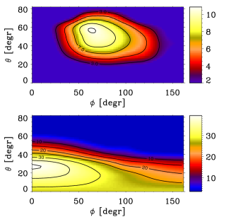
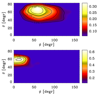
Figure 4: Vertical fluxes measured at the top of the atmosphere at 1 Mm for waves with $\nu=5$ mHz (left panels) and 3 mHz (right panels). Upper panels give magnetic fluxes and lower panels give acoustic fluxes.

Finally, Figure 4 gives the time averages of the vertical magnetic and acoustic fluxes at the top of the atmosphere as a function of the field orientation. As proven above, the magnetic flux at 1 Mm corresponds to the Alfvén mode. At $\nu=5$ mHz, the maximum of the magnetic flux corresponds to $\theta=50^{\circ}$ and $\phi=65^{\circ}$. This maximum is shifted to larger inclinations $\theta=65^{\circ}$ for waves with $\nu=3$ mHz. The presence of the sharp maximum of the Alfvénic flux transmission agrees well with the conclusions made previously by Cally & Goossens [8], though the exact position of the maximum is shifted to somewhat larger inclinations. The maximum of the transmitted acoustic flux corresponds to inclinations $\theta\approx 30^{\circ}$ for $\nu=5$ mHz waves, and to $\theta\approx 55^{\circ}$ for $\nu=3$ mHz waves, again, in agreement with previous calculations [3, 8]. The absolute value of the fluxes is about 30 times lower for 3 mHz compared to 5 mHz. At some angles the Afvén magnetic flux transmitted to the upper atmosphere is larger than the acoustic flux. However, at angles corresponding to the maximum of the transmission, the Alfvén flux is 2-3 times lower than the corresponding acoustic flux.

It is important to realize that quantitatively simulating mode transformation numerically is a challenge, as any numerical inaccuracies are amplified in such second-order quantities as wave energy fluxes. The tests presented in this paper prove the robustness of our numerical procedure and offer an effective way to separate the Alfvén from magneto-acoustic modes in numerical simulations. This will allow us in future to study the coupling between magneto-acoustic and Alfvén waves in more realistic situations resembling complex solar magnetic structures.

References

References

- [1] Zhugzhda Y D and Dzhalilov N S 1982 Astron. Astrophys. 112 16
- [2] Cally P S and Bogdan T J 1997 Apj 486 L67
- [3] Schunker H and Cally P S 2006 MNRAS 372 551
- [4] Cally P S 2006 Phil. Trans. R. Soc. A 364 333
- [5] Khomenko E, Kosovichev A, Collados M, Parchevsky K and Olshevsky V 2009 Apj 694 411
- [6] Felipe T, Khomenko E and Collados M 2010 Apj 719 357
- [7] Khomenko E 2009 ASP Conf. Series vol 416 ed. M Dikpati, T Arentoft, I González Hernández, C Lindsey, & F Hill p. 31
- [8] Cally P S and Goossens M 2008 Solar Phys. 251 251
- [9] Newington M E and Cally P S 2010 MNRAS 402 386
- [10] Khomenko E and Collados M 2006 Apj 653 739
- [11] Khomenko E, Centeno R, Collados M and Trujillo Bueno J 2008 Apj 676 L85
- [12] Priest E R 1984 Solar magneto-hydrodynamics Geophysics and Astrophysics Monographs, Dordrecht: Reidel