Abstract

We exploit the symmetry concepts developed in the companion review of this article to introduce a stochastic version of link reversal symmetry, which leads to an improved understanding of the reciprocity of directed networks. We apply our formalism to the international trade network and show that a strong embedding in economic space determines particular symmetries of the network, while the observed evolution of reciprocity is consistent with a symmetry breaking taking place in production space. Our results show that networks can be strongly affected by symmetry-breaking phenomena occurring in embedding spaces, and that stochastic network symmetries can successfully suggest, or rule out, possible underlying mechanisms.

10.3390/—— xx Received: xx / Accepted: xx / Published: xx Complex Networks and Symmetry II: Reciprocity and Evolution of World Trade Franco Ruzzenenti ^1,⋆, Diego Garlaschelli ² and Riccardo Basosi ³ E-Mail: ruzzenenti@unisi.it; Tel.: +39-0577-234240; Fax: +39-0577-234239.

1 Introduction

In this paper, we take full advantage to the symmetry concepts developed in the companion review symmetry1 in order to study in great detail two applications of stochastic symmetry in networks. First, we discuss link reversal symmetry in directed networks and introduce its stochastic variant to highlight the connections with the important property of reciprocity. Second, we consider the problem of (stochastic) symmetry breaking in spatially embedded networks (where the embedding space is in general not necessarily Euclidean or geographic, but specified by different variables). Both applications will be discussed in the context of an empirical analysis of a particular network: the World Trade Web, defined by the international trade relationships existing among all world countries.

The investigation of symmetry naturally leads to the fascinating problem of symmetry breaking. ‘All scientific applications of symmetry are based on the principle that identical causes produce identical effects’ 1 . That is to say, the symmetry of the effect must be at least that of the cause, or in a mathematical jargon: the order of the symmetry group of the effect must be at least equivalent to that of the cause. Nevertheless, for a qualitatively new phenomenon to occur, symmetry cannot be conserved. Pierre Curie was the first in modern science who highlighted the relevance of spontaneous symmetry breaking in various phenomena 2 . His studies of criticality in phase transitions overcame the boundaries of solid state physics and posed a suitable analytical framework for further studies, in different fields. Prigogine himself, a renowned and illustrious precursor of complex systems research, referred to Curie’s contribution in order to elucidate the meaning of symmetry breaking in dissipative structures: ‘We see therefore, that the appearance of a periodic reaction is a time-symmetry breaking process exactly as ferromagnetism is a space-symmetry breaking one’ 3 . Two main viewpoints on symmetry breaking developed in science: one concerned with space symmetry and one with time symmetry. Symmetry breaking can be indeed approached from two different sides: from a time-scale perspective, as we see the phenomenon as a dynamic system, or from a spatial perspective, as we focus on changes in the system’s space. With the former approach we tend to consider changes that are endogenous to the system, while space is taken as homogeneous all the way through; with the latter, the system is embedded in some space and changes are considered exogenous. However, whereas in physics space-symmetry breaking has been a prominent research subject, in the field of complex nonlinear systems time-symmetry breaking has received much more attention. The following passage by Mainzer illustrates on what basis time symmetry breaking became a major topic in the science of complexity: ‘Thus, bifurcation mathematically only means the emergence of new solutions of equations at critical values. Actually, bifurcation and symmetry breaking is a purely mathematical consequence of the theory of nonlinear differential equations. But, bifurcations of final states as solutions of differential equations correspond to qualitative changes of dynamical systems and the emergence of new phenomena in nature and society [..]’4 .

In what follows, spatial symmetry breaking will be approached in the framework of complex networks. Symmetries relevant to networks can be either ‘internal’, if they involve purely topological quantities, or ‘external’, if they are defined with respect to additional properties such as positions in some embedding space. In the latter case, symmetries relative to the external space can be reflected in some topological property displayed by the network symmetry1 . In this sense, spatial symmetry breaking has so far received little attention in the field of network theory, despite the latter developed considerably in recent years guidosbook ; largescalestructure ; dynamicalprocessesoncomplexnetworks ; ecologicalnetworks ; internet ; networksincellbiology ; adaptivenetworks . On the other hand, specific analyses of processes that are well described within a network framework suggest that spatial symmetry breaking can occur with respect to some embedding space and manifest itself in major structural changes at a topological level, as happened in the evolution of vascular systems in living beings west , of river basins banavar , and of production networks in modern economies 7 ; 8 . In the present paper, we exploit our review of network symmetries symmetry1 to start investigating this problem. The paper is organized as follows. In Section 2 we will introduce link reversal symmetry and we define a new stochastic variant of it. In Section 3 we will then investigate how stochastic link reversal symmetry, together with other symmetries discussed in referencsymmetry1 , enable to achieve an improved understanding of network structure in a specific case, i.e. the problem of reciprocity in directed networks. We will highlight how different measures of reciprocity capture different symmetry properties of a network. This will help us disentangle distinct possible mechanisms explaining the observed reciprocity structure of real networks. As a particular application, in Section 5 we will consider the evolution of reciprocity in the World Trade Web. We will also emphasize the role of spatial embedding, which relates the topology of the network to underlying geographical coordinates and economic variables. We will advance heuristic explanations for the observed evolution of reciprocity in the World Trade Web in terms of symmetry breaking phenomena due to changes in the underlying economic structure. These analyses highlights the idea that complex networks are not phenomena per se, but maps of physical phenomena that are immersed in physical space—or any other space, depending on the variables determining the system’s dynamics. Symmetry breaking can occur in some geographical, economic, or different space, and be mirrored in the topological space the network belongs to. In real imperfect systems, stochastic symmetry is able to capture spatial patterns that are undetected by exact symmetries. Interactions between the underlying system’s ‘spaces’ is an intriguing challenge for network theory and pertains the study of network dynamics.

2 Exact and Stochastic Link Reversal Symmetry

In this section we make use of the notion of stochastic graph symmetries we introduced in Reference symmetry1 to define a new graph invariance, i.e. the stochastic version of link reversal symmetry. To this end, we first briefly recall the concept of graph ensembles and equiprobability symmetry1 , and then discuss link reversal symmetry, first in its exact version and finally in its stochastic variant.

2.1 Graph Ensembles and Stochastic Symmetries

In Reference symmetry1 we introduced the concept of graph ensembles as collections of graphs with specified properties and probability. Each graph $G$ in a statistical ensemble of graphs has an associated occurrence probability $P(G)$ satisfying

$$\sum_{G}P(G)=1$$ (1)

Two graphs $G_{1}$ and $G_{2}$ such that $P(G_{1})=P(G_{2})$ are said to be equiprobable in the ensemble considered. The probability $P(G)$ can have different forms depending on the structure of the ensemble under consideration. In what follows, we will make use of (grand)canonical ensembles, and in particular maximally random graphs with specified constraints symmetry1 . Such ensembles are defined by specifying the expected value (ensemble average) of a chosen set of topological properties (the constraints), and are maximally random otherwise. This means that the probability $P(G)$ must maximize the entropy of the ensemble subject to the enforced constraints. The constraints will be denoted as a collection $\{c_{1},\dots,c_{K}\}$ of $K$ topological properties, and the Lagrange multipliers involved in the constrained maximization problem will be denoted as the conjugate parameters $\{\theta_{1},\dots,\theta_{K}\}$. The probability $P(G)$ will depend on such parameters, and its explicit form is

$$P(G)=\frac{e^{-H(G)}}{Z}$$ (2)

where $H(G)$ is the graph Hamiltonian

$$H(G)\equiv\sum_{a=1}^{K}\theta_{a}c_{a}(G)$$ (3)

and $Z$ is the partition function

$$Z\equiv\sum_{G}e^{-H(G)}$$ (4)

The expected value of a topological property $X$, which evaluates to $X(G)$ on the particular graph $G$, is

$$\langle X(\theta_{1},\dots,\theta_{K})\rangle\equiv\sum_{G}P(G)X(G)$$ (5)

The values of the parameters $\{\theta_{1},\dots,\theta_{K}\}$ are such that the expected values $\{\langle c_{1}\rangle,\dots,\langle c_{K}\rangle\}$ of the constraints match the specified values. In particular, if the ensemble is meant as a null model symmetry1 of a real network $G^{*}$, the expected values of the constraints will have to match the empirical values of the properties $\{c_{1}(G^{*}),\dots,c_{K}(G^{*})\}$ of that particular graph:

$$\langle c_{a}(\theta^{*}_{1},\dots,\theta^{*}_{K})\rangle=c_{a}(G^{*})\qquad a=1,\dots,K$$ (6)

The above parameter choice automatically maximises the probability $P(G^{*})$ to obtain the real network $G^{*}$ under the model considered, and is therefore in accordance with the maximum likelihood principle mylikelihood . The graph Hamiltonian $H(G)$, which represents a sort of energy or cost associated to the graph $G$, is a linear combination of the constraints. Clearly, $P(G_{1})=P(G_{2})$ if and only if $H(G_{1})=H(G_{2})$, which means that graphs with the same energy are equiprobable (and vice versa). The transformation mapping $G_{1}$ into a different graph $G_{2}$ with $H(G_{2})=H(G_{1})$ is a symmetry of the Hamiltonian. Any such transformation changes the topology of the graph but preserves the values of the constraints appearing in the Hamiltonian (and is therefore more general than permutations of vertices).

Graph ensembles provide an ideal framework to study stochastic graph symmetries, that we defined in Reference symmetry1 . An exact symmetry of a real network $G^{*}$ is a transformation mapping $G^{*}$ to itself (for instance, an automorphism if the transformation considered is a vertex permutation symmetry ; quotient ; redundancy ; symmetry_wtw ). By contrast, a stochastic symmetry is associated with an ensemble of graphs, rather than with a single one. In particular, we can define a graph ensemble as stochastically symmetric under a transformation if the latter maps each graph $G_{1}$ into an equiprobable subgraph $G_{2}$ with $P(G_{1})=P(G_{2})$. Maximally random graphs with constraints are therefore stochastically symmetric under transformations that are symmetries of the Hamiltonian. If a real network $G^{*}$ is well reproduced by a stochastically symmetric ensemble, then we can denote $G^{*}$ as stochastically symmetric (under the same transformations involved in the symmetry of the ensemble, or under the model considered for brevity). That is, while $G^{*}$ is exactly symmetric under its automorphisms, it is stochastically symmetric under the transformations defining an ensemble of which $G^{*}$ is a typical member. By contrast, if the ensemble is not a good model of the real network,then those transformations are not stochastic symmetries of $G^{*}$. We will encounter both situations later on.

Two important examples of maximally random graphs that we will use as null models are the Erdős-Rényi random graph model and the configuration model. Here we consider the undirected versions of both models, and we will generalize them to the directed case later on. To avoid confusion with their directed counterparts, here we use a different notation with respect to our presentation in Reference symmetry1 . The adjacency matrix of an undirected graph will be denoted as $B$, with entries $b_{ij}=1$ if an undirected link between vertices $i$ and $j$ is there, and $b_{ij}=0$ otherwise.

In the undirected Erdős-Rényi random graph model, the only constraint is the total number of undirected links $L^{u}=\sum_{i<j}b_{ij}$. Thus the Hamiltonian reads

$$H(G)=\theta L^{u}(G)$$ (7)

and its symmetries are the transformations mapping a graph $G$ into another (equiprobable) graph with the same number of links. The probability $P(G)$ factorizes in terms of the probability

$$q\equiv\frac{e^{-\theta}}{1+e^{-\theta}}$$ (8)

that a link is there between any two vertices. If the model is interpreted as a null model of the real network $G^{*}$, the parameter $q$ must be set to the particular value $q^{*}$ such that

$$\langle L^{u}\rangle=q^{*}\frac{N(N-1)}{2}=L^{u}(G^{*})$$ (9)

ensuring that, in accordance with the maximum likelihood principle mylikelihood , the expected number of links $\langle L^{u}\rangle$ coincides with the number of links $L^{u}(G^{*})$ of $G^{*}$.

In the configuration model, the constraints are the degrees of all vertices, i.e. the degree sequence $\{k_{i}\}$, where $k_{i}\equiv\sum_{j\neq i}b_{ij}$. Therefore the Hamiltonian takes the form

$$H(G)=\sum_{i=1}^{N}\theta_{i}k_{i}(G)$$ (10)

and its symmetries are the transformations that map a graph into a different one with the same degree sequence, i.e. those explored by the local rewiring algorithm symmetry1 . The probability that vertices $i$ and $j$ are connected is no longer uniform across all pairs of vertices, and reads

$$q_{ij}=\frac{w_{i}w_{j}}{1+w_{i}w_{j}}$$ (11)

where $w_{i}\equiv e^{-\theta_{i}}$. If the configuration model is used as a null model of a real network $G^{*}$, then the parameters $\{w_{1},\dots,w_{N}\}$ must be set to the values $\{w^{*}_{1},\dots,w^{*}_{N}\}$ solving the following $N$ coupled equations

$$\langle k_{i}\rangle=\sum_{j\neq i}\frac{w^{*}_{i}w^{*}_{j}}{1+w^{*}_{i}w^{*}_{j}}=k_{i}(G^{*})\qquad\forall i$$ (12)

ensuring that the expected degree sequence coincides with the observed one, and maximising the likelihood to obtain $G^{*}$ mylikelihood ; myrandomization .

2.2 Transpose Equivalence and Transpose Equiprobability

We now come to the description of link reversal symmetry. There are two ways in which one can formulate link reversal symmetry in directed networks. The first, simpler definition is the exact invariance of a single graph under the inversion of the direction defined on each of its edges. Under this definition, the graph is perfectly symmetric if all of its edges are bidirectional. If $A$ is the adjacency matrix of a directed graph ($a_{ij}=1$ if a directed edge from $i$ to $j$ is there, and $a_{ij}=0$ otherwise), then the graph is exactly symmetric under link reversal if

$$A=A^{T}$$ (13)

where $A^{T}$ indicates the transpose of the matrix $A$. Clearly, bidirectional graphs are equivalent to undirected graphs. In this sense, one can say that real networks are found to be either symmetric (this is the case of real-world undirected networks such as the Internet, protein interaction graphs or friendship networks) or asymmetric (this is the case of intrinsically directed networks such as food webs, the WWW, metabolic networks, the World Trade Web, etc.). This first type of link reversal symmetry will be denoted transpose equivalence in what follows.

A second, novel definition of link reversal symmetry that we introduce here is a stochastic one, in the sense discussed in Reference symmetry1 and briefly recalled above. As any stochastic symmetry, it is associated to an ensemble of equiprobable graphs. If each graph $G$ in the ensemble is identified with its adjacency matrix $A$, we say that the ensemble is stochastically symmetric under link reversal if

$$P(A)=P(A^{T})$$ (14)

This second definition is completely different from the first one. It does not imply that any single graph $A$ in the ensemble is bidirectional, but that it has the same probability of occurrence of its link-reversed $A^{T}$, i.e. $P(A)=P(A^{T})$. The equiprobability of $A$ and $A^{T}$ has important effects on the directionality of the expected topological properties across the ensemble, but is perfectly consistent with the asymmetry of individual graphs in the ensemble. If the ensemble considered is a maximally random graph model defined by a Hamiltonian $H(G)$ (see Section 2.1), then Equation (14) is equivalent to

$$H(A)=H(A^{T})$$ (15)

showing that link reversal is a symmetry of the Hamiltonian. In accordance with our general definition of stochastic symmetry symmetry1 recalled in Section 2.1, we can also define a single graph $G^{*}$ as stochastically symmetric under link reversal if it is a typical member of (i.e. it is well modelled by) an ensemble which is stochastically symmetric under link reversal. In simpler words, the graph $A$ is stochastically symmetric under link reversal if it is statistically equivalent to its link-reversed $A^{T}$. This second, stochastic type of link reversal symmetry will be denoted transpose equiprobability in what follows.

The dichotomy existing between transpose equivalence and transpose equiprobability, the different underlying mechanisms they might reveal, and the relation they have to many of the symmetries we have discussed in Reference symmetry1 (including ensemble equiprobability, statistical equivalence and dependence on external or hidden vertex properties) make link reversal symmetry an ideal candidate to discuss in more detail in what follows. Moreover, link reversal symmetry is tightly related to the problem of reciprocity. Therefore, before presenting a deeper study of this symmetry, in the next section we study the problem of reciprocity in great detail.

3 Reciprocity of Directed Networks

Reciprocity is the tendency of pairs of vertices to be connected by two mutual links pointing in opposite directions, a particular type of correlation found in directed networks wasserman ; myreciprocity ; mymultispecies . Depending on the nature of the network, reciprocity is related to various important phenomena, such as ecological symbiosis in food webs, reversibility of biochemical reactions in metabolic networks, bidirectionality of chemical synapses in neural networks, synonymy in networks of dictionary terms, mutuality of psychological associations in networks of freely linked words, reciprocity of hyperlinks in the WWW, crossed financial ownership in shareholding networks, economic interdependence of countries in the international trade network, and so on myreciprocity . In this section, we study link reversal symmetry in great detail. We first discuss the problem of the definition of proper reciprocity measures, present the analysis of the reciprocity structure of real networks, and define some theoretical concepts useful to interpret the observed patterns. Then, in Section 4 we highlight the relation existing between reciprocity, the two types of link reversal symmetry defined in Section 2.2, and other symmetries we introduced. In Section 5 we finally apply all these concepts to the empirical analysis of the World Trade Web.

3.1 The Traditional Approach to Reciprocity

The study of reciprocity has a long tradition in social science wasserman as a way to quantify how many ‘ties’ (directed links) are reciprocated in a social network of ‘actors’ (vertices). The reciprocal link of a directed link pointing from $i$ to $j$ is a link pointing from $j$ to $i$. A link is reciprocated if its reciprocal one is present in the network. In terms of the adjacency matrix of the graph, two reciprocated links are present between $i$ and $j$ if and only if $a_{ij}=a_{ji}=1$. In the example shown in Figure 1a, the edges between vertices $A$ and $B$, as well as those between $A$ and $D$, are reciprocated. All other edges are not reciprocated. Therefore, while the total number of directed links is given by

$$L=\sum_{i\neq j}a_{ij}$$ (16)

the number of reciprocated links is

$$L^{\leftrightarrow}=\sum_{i\neq j}a_{ij}a_{ji}$$ (17)

Since $0\leq L^{\leftrightarrow}\leq L$, the traditional definition of the reciprocity of a network is

$$r\equiv\frac{L^{\leftrightarrow}}{L}$$ (18)

so that $0\leq r\leq 1$. Although not usually remarked, it is important to notice that whether the value of $r$ can actually span the entire range between $0$ and $1$ depends on the link density (or connectance) of the network, defined as

$$\bar{a}\equiv\frac{\sum_{i\neq j}a_{ij}}{N(N-1)}=\frac{L}{N(N-1)}$$ (19)

We shall comment more about the effects of $\bar{a}$ on the allowed values of the reciprocity later on. Note that the requirement $i\neq j$ in Equations (16), (17) and (19) arises from the assumption of no self-loops (links starting and ending at the same vertex) in the network. If self-loops are present, we assume that they are ignored and therefore not computed in $L$ and $L^{\leftrightarrow}$. This is because self-loops would give a nonzero contribution to both $L$ and $L^{\leftrightarrow}$, even if they are not a true signature of reciprocity. Two networks with the same topology apart from a different number of self-loops should not be considered as having different degrees of reciprocity myreciprocity .

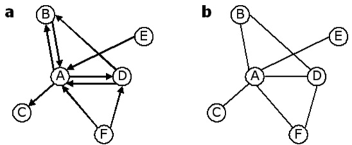
Figure 1: (a) Example of a directed network with $N=6$ vertices. Here $L=9$, $L^{\leftrightarrow}=4$ and the maximum possible number of directed links is $N(N-1)=30$. (b) The undirected version of the same network. Here $L^{u}=7$ and the maximum possible number of undirected links is $N(N-1)/2=15$.

As for any topological property, a given value of $r$ is only significant with respect to some null model. This is because, even in a network where directed links are drawn completely at random, a certain number of reciprocated connections will be formed. As we shall discuss in more detail in Section 4, in such an uncorrelated network $r$ is simply equal to the average probability that any two vertices are connected by a directed link, i.e. to the connectance defined in Equation (19):

$$r_{rand}=\bar{a}$$ (20)

Comparing the value of $r$ with that of $r_{rand}$ allows to assess if mutual links occur more ($r>r_{rand}$) or less ($r<r_{rand}$) often than expected by chance. This is the traditional approach to the study of reciprocity in social networks, which has been more recently extended to other networks such as the WWW, e-mail networks and the World Trade Web myreciprocity .

3.2 An Improved Definition

Although the comparison of $r$ with $r_{rand}$ is a safe method to detect nonrandom reciprocity in a particular network, it is completely unadapted to compare the reciprocity of networks with different link density, or to assess the evolution of reciprocity in a single network with time-varying density myreciprocity . This is because $r$ is not an absolute quantity, and its value has only a relative meaning with respect to $r_{rand}=\bar{a}$. The reference value for $r$ unavoidably varies as the density $\bar{a}$ varies. Therefore it is not possible to order various networks, or various snapshots of the same network, according to their value of $r$. In order to overcome this problem, a new definition of reciprocity was proposed myreciprocity as the Pearson correlation coefficient between the symmetric entries of the adjacency matrix:

$$\rho\equiv\frac{\sum_{i\neq j}(a_{ij}-\bar{a})(a_{ji}-\bar{a})}{\sum_{i\neq j}(a_{ij}-\bar{a})^{2}}=\frac{r-\bar{a}}{1-\bar{a}}$$ (21)

where the second equality comes from an explicit calculation making use of Equations (16)– (18) and of the property ${(a_{ij})^{2}=a_{ij}}$. The range of $\rho$, as for any correlation coefficient, is $-1\leq\rho\leq 1$ (see however our discussion below for more details on the allowed values of $\rho$). It is possible to write down an expression for the statistical error associated to a single measurement of $\rho$ on a particular network myreciprocity .

Unlike $r$, $\rho$ is an absolute quantity, and the effects of link density are already accounted for in it. In particular, its null value is

$$\rho_{rand}=0$$ (22)

irrespective of the value of $\bar{a}$. The sign of $\rho$ alone is enough to distinguish between positively correlated (or reciprocal) networks where there are more reciprocated links than expected by chance ($\rho>0$) and negatively correlated (or antireciprocal) networks where there are fewer reciprocated links than expected by chance ($\rho<0$). The null case $\rho=0$ (consistently with the statistical error) corresponds to uncorrelated or areciprocal networks. The existence of a unique reference scale allows to order several networks according to their value of $\rho$, as shown in Table 1. Among the networks considered, one finds both positively and and negatively correlated ones. Remarkably, such ordering reveals interesting empirical patterns of reciprocity, since networks of the same kind are found to display similar values of $\rho$. The positively correlated networks are, in decreasing order of $\rho$ (see Table 1): all purely bidirectional (undirected) networks such as the Internet ($\rho=1$), the 53 snapshots of the World Trade Web from year 1948 to 2000 ($0.68\leq\rho\leq 0.95$), an instance of the WWW ($\rho=0.5165$), two neural networks ($0.41\leq\rho\leq 0.44$), two e-mail networks ($0.19\leq\rho\leq 0.23$), two word association networks ($0.12\leq\rho\leq 0.19$) and 43 metabolic networks ($0.006\leq\rho\leq 0.052$). In particular, for the 53 snapshots of the World Trade Web considered, the use of $\rho$ allows to properly track the evolution of reciprocity over time, as we shall discuss in Section 5. The negatively correlated networks considered are two shareholding networks ($-0.0034\leq\rho\leq-0.0012$) and 28 food webs ($-0.13\leq\rho\leq-0.01$). The case of minimum reciprocity will be discussed in Section 3.3.

The analysis reported above reveals that real networks display nontrivial reciprocity patterns and are always either correlated or anticorrelated. This result is very important, since theoretical studies have shown that a nontrivial degree of reciprocity affects the properties of various dynamical processes taking place on directed networks, such as epidemic spreading recipr_newman , percolation recipr_boguna , and localization recipr_vinko . The effects of reciprocity are even more interesting on scale-free networks, where even an infinitely small fraction of bidirectional links was shown to give rise to a phase transition characterized by the onset of a giant strongly connected component recipr_boguna .

3.3 Minimum Reciprocity

As we mentioned, in principle the allowed range of $\rho$ is ${-1\leq\rho\leq 1}$. However, from Table 1 we note that while the most correlated directed network in the set considered displays $\rho=0.95$, which is almost equal to the largest possible value, the most anticorrelated one displays only $\rho=-0.13$, which is quite far from the lower bound $\rho=-1$. Still, for most of the 30 antireciprocal networks reported in the table the number of reciprocated links is zero ($r=0$) and therefore the value of $\rho$ is the minimum possible myreciprocity .

Network	Range of $\rho$
Perfectly reciprocal	$\rho=1$
World Trade Web (53 webs)	$0.68\leq\rho\leq 0.95$
World Wide Web (1 web)	$\rho=0.5165$
Neural Networks (2 webs)	$0.41\leq\rho\leq 0.44$
Email Networks (2 webs)	$0.19\leq\rho\leq 0.23$
Word Networks (2 webs)	$0.12\leq\rho\leq 0.19$
Metabolic Networks (43 webs)	$0.006\leq\rho\leq 0.052$
Areciprocal	$\rho=0$
Shareholding Networks (2 webs)	$-0.0034\leq\rho\leq-0.0012$
Food Webs (28 webs)	$-0.13\leq\rho\leq-0.01$
Perfectly antireciprocal	$\rho=-1$

Table 1: Empirical values of $\rho$ (in decreasing order), for the 133 real networks analysed in Reference myreciprocity . The values reported show the significant digits with respect to the statistical errors.

This seemingly puzzling outcome can be explained as follows. Note that Equation (21) implies that even in a network with $r=0$ the value of $\rho$ is always different from $-1$ unless $\bar{a}=1/2$. This occurs because $\bar{a}=1/2$ is the only case allowing perfect anticorrelation: in order to have $a_{ij}=1$ whenever $a_{ji}=0$, the adjacency matrix must be exactly ‘half-filled’ with unit entries, and the number of links must be half the maximum possible one myreciprocity . Remarkably, for $\bar{a}\neq 1/2$ there are two different cases. In the ‘sparse’ range $\bar{a}<1/2$, the minimum value of $r$ is $r_{min}=0$ since it is always possible to place all the links without having reciprocal pairs. Consequently, Equation (21) implies that ${\rho_{min}=\bar{a}/(\bar{a}-1)}$. By contrast, in the ‘dense’ range $\bar{a}>1/2$ some links must be unavoidably placed between the same pairs of vertices and therefore $r>0$. More precisely, since the number of vertex pairs is ${N(N-1)/2}$, the minimum number of reciprocal links is given by twice the number of links exceeding this number, or in other words ${L^{\leftrightarrow}_{min}=2[L-N(N-1)/2]}$. Consequently, ${r_{min}=2-1/\bar{a}}$ and ${\rho_{min}=(\bar{a}-1)/\bar{a}}$. Putting these results together, we have

$$r_{min}=\left\{\begin{array}[]{ll}0&\quad\textrm{if $\bar{a}\leq 1/2$}\\ &\\ 2-\displaystyle\frac{1}{\bar{a}}&\quad\textrm{if $\bar{a}>1/2$}\end{array}\right.$$ (23)

and

$$\rho_{min}=\left\{\begin{array}[]{ll}\displaystyle\frac{\bar{a}}{\bar{a}-1}&\quad\textrm{if $\bar{a}\leq 1/2$}\\ &\\ \displaystyle\frac{\bar{a}-1}{\bar{a}}&\quad\textrm{if $\bar{a}>1/2$}\end{array}\right.$$ (24)

Both trends, together with the simple behaviour of $r_{rand}=\bar{a}$ for an antireciprocal network, are shown as functions of $\bar{a}$ in Figure 2.

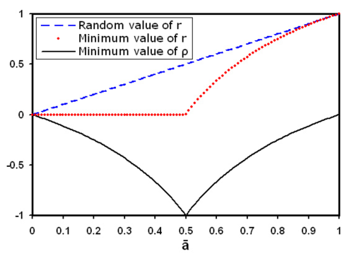
Figure 2: Behaviour of $r_{rand}$, $r_{min}$ and $\rho_{min}$ as functions of $\bar{a}$.

3.4 Related Topological Properties

In this section we introduce various topological properties related to the reciprocity of a network. We will refer again to Figure 1 to illustrate many of the properties discussed in this section. The local quantities that characterize each vertex $i$ are the in-degree $k^{in}_{i}$ and the out-degree $k^{out}_{i}$, defined as the number of in-coming and out-going links respectively:

$$k^{in}_{i} = \sum_{j\neq i}a_{ji}$$ (25)

$$k^{out}_{i} = \sum_{j\neq i}a_{ij}$$ (26)

In the example shown in Figure 1a, vertex $A$ has $k^{in}_{A}=4$ in-coming links and $k^{out}_{A}=3$ out-going links. Unfortunately, these commonly used quantities do not carry information about the reciprocity, since they do not tell us if the in-coming and out-going links of a vertex $i$ ‘overlap’ completely, partly or not at all. As a way to measure the overlap between the sets of in-coming and out-going links of a vertex $i$, the reciprocated degree $k^{\leftrightarrow}_{i}$ was defined myreciprocity ; mymultispecies ; recipr_newman ; recipr_boguna as the number of ‘reciprocal neighbours’ (vertices joined by two reciprocal links) of $i$:

$$k^{\leftrightarrow}_{i}\equiv\sum_{j\neq i}a_{ij}a_{ji}$$ (27)

In the example shown in Figure 1a, vertex $A$ has $k^{\leftrightarrow}_{A}=2$ reciprocal neighbours. As extreme examples, in a purely bidirectional network ($\rho=1$) there is complete overlap and ${k^{\leftrightarrow}_{i}=k^{in}_{i}=k^{out}_{i}\ \forall i}$, while in a purely unidirectional network ($\rho=\rho_{min}<0$) there is no overlap and ${k^{\leftrightarrow}_{i}=0\ \forall i}$. One could think of $k^{\leftrightarrow}_{i}$ as the result of a kind of ‘attraction’ or ‘repulsion’ between the in-coming and out-going links of vertex $i$, and of $\rho$ as an average strength of the corresponding (positive or negative) interaction.

As we mentioned, the knowledge of $k^{in}_{i}$ and $k^{out}_{i}$ alone is not enough to know $k^{\leftrightarrow}_{i}$. It only informs us about the maximum possible overlap, which is

$$(k^{\leftrightarrow}_{i})_{max}=\min\{k^{in}_{i},k^{out}_{i}\}$$ (28)

In the case shown in Figure 1a, $(k^{\leftrightarrow}_{A})_{max}=3$. If the total number $N$ of vertices is known, then $k^{in}_{i}$ and $k^{out}_{i}$ can also tell us about the minimum overlap, which is

$$(k^{\leftrightarrow}_{i})_{min}=\left\{\begin{array}[]{ll}0&\quad\textrm{if}\ k^{in}_{i}+k^{out}_{i}\leq N-1\\ k^{in}_{i}+k^{out}_{i}-(N-1)&\quad\textrm{if}\ k^{in}_{i}+k^{out}_{i}>N-1\end{array}\right.$$ (29)

depending on the possibility to place in-coming and out-going links without overlap. The above expression is the analogous of Equation (23) for individual vertices. In the case shown in Figure 1a, $(k^{\leftrightarrow}_{A})_{min}=2$. Indeed, in the example considered it would be impossible to achieve a value of $k^{\leftrightarrow}_{A}$ smaller than that realised, given the values of $k^{in}_{A}$ and $k^{out}_{A}$. It would also be impossible to achieve a value of $k^{\leftrightarrow}_{A}$ larger than $3$. In general, even the joint knowledge of the in- and out-degrees $\{k^{in}_{i}\}$ and $\{k^{out}_{i}\}$ of all vertices, or similarly the joint degree distribution $P(k^{in}=k,k^{out}=k^{\prime})$ that a randomly chosen vertex has in-degree $k$ and out-degree $k^{\prime}$, cannot characterize the reciprocity of the network. What can be extracted from these quantities is only the maximum and minimum numbers of reciprocated links, an information analogous to that leading to Equation (24).

By contrast, the three degree sequences $\{k^{in}_{i}\}$, $\{k^{out}_{i}\}$ and $\{k^{\leftrightarrow}_{i}\}$ specify the connectivity properties including the reciprocity. Summing over all vertices gives the same information as Equations (16) and (17), and $\rho$ can then be easily computed. Alternatively, it is also possible to define the non-reciprocated in-degree $k^{\leftarrow}_{i}$ and the non-reciprocated out-degree $k^{\to}_{i}$ of a vertex $i$ as the number of in-coming and out-going links that are not reciprocated respectively:

$$k^{\leftarrow}_{i} \equiv \sum_{j\neq i}a_{ji}(1-a_{ij})=k^{in}_{i}-k^{\leftrightarrow}_{i}$$ (30)

$$k^{\to}_{i} \equiv \sum_{j\neq i}a_{ij}(1-a_{ji})=k^{out}_{i}-k^{\leftrightarrow}_{i}$$ (31)

In the example shown in Figure 1a, vertex $A$ has $k^{\leftarrow}_{A}=2$ and $k^{\to}_{A}=1$. The information specified by the three degree sequences $\{k^{\leftarrow}_{i}\}$, $\{k^{\to}_{i}\}$ and $\{k^{\leftrightarrow}_{i}\}$ is the same as that carried by $\{k^{in}_{i}\}$, $\{k^{out}_{i}\}$ and $\{k^{\leftrightarrow}_{i}\}$. Note that the total degree $k^{tot}_{i}$ can be expressed in the equivalent forms

$$k^{tot}_{i} = \sum_{j\neq i}(a_{ji}+a_{ij})$$

$$= k^{in}_{i}+k^{out}_{i}$$

$$= k_{i}^{\leftarrow}+k_{i}^{\to}+2k_{i}^{\leftrightarrow}$$

The above quantities also come into play whenever a directed graph is regarded as an undirected one by simply ignoring the direction of the links. We will consider this problem in a real-world case in Section 5. The undirected projection of a directed graph is an undirected graph where each pair of vertices is connected by an undirected edge if at least one directed link (irrespective of its direction) is present between them in the original directed graph. Figure 1b reports the undirected version of the directed graph of Figure 1a. If $A$ is the adjacency matrix of the original directed network, then the adjacency matrix $B$ of the projected undirected network has entries

$$b_{ij}=a_{ij}+a_{ji}-a_{ij}a_{ji}$$ (33)

and is now symmetric, as for any undirected network. Each vertex $i$ in the undirected graph is now simply characterized by its undirected degree $k_{i}$:

$$k_{i} = \sum_{j\neq i}b_{ji}$$

$$= k^{in}_{i}+k^{out}_{i}-k^{\leftrightarrow}_{i}$$

$$= k^{\leftarrow}_{i}+k^{\to}_{i}+k^{\leftrightarrow}_{i}$$

The number of links $L^{u}$ in the undirected network is

$$L^{u}=\sum_{i<j}b_{ij}=\frac{1}{2}\sum_{i}k_{i}=L-\frac{1}{2}L^{\leftrightarrow}=\left(1-\frac{r}{2}\right)L$$ (35)

and the link density, or connectance, of the undirected network is the ratio between $L^{u}$ and the maximum number of undirected links, i.e.

$$\bar{b}\equiv\frac{2\sum_{i<j}b_{ij}}{N(N-1)}=\frac{2L^{u}}{N(N-1)}=(2-r)\bar{a}$$ (36)

which is in an interesting relation with Equation (19). From the above equations, which can be checked explicitly in the example shown in Figure 1, it is clear that the knowledge of $k^{in}_{i}$ and $k^{out}_{i}$ is not enough to determine $k_{i}$. Again, a crucial role is played by $k^{\leftrightarrow}_{i}$ and consequently by the reciprocity of the network. For perfectly antireciprocal networks $k^{\leftrightarrow}_{i}=0$ and $k_{i}=k^{tot}_{i}$, while for perfectly reciprocal ones $k_{i}=k^{\leftrightarrow}_{i}=k^{tot}/2$. More in general, the knowledge of a directed topological property is not enough to determine the corresponding property in the projected undirected graph. The missing information is carried by the reciprocity structure of the network.

In what follows, it will be useful to evaluate the expectation values of the above quantities across various graph ensembles. Therefore, before discussing specific cases, we briefly develop a formalism useful in an ensemble setting. In a graph ensemble, each link has an associated probability of occurrence symmetry1 . The information relevant to the reciprocity structure is captured by two different probabilities. The first one is the marginal probability

$$p_{ij}\equiv p(i\to j)=\langle a_{ij}\rangle$$ (37)

that a directed link from $i$ to $j$ is there, irrespective of the presence of the reciprocal link. The second one is the conditional probability $r_{ij}$ that a directed link from vertex $i$ to vertex $j$ is there given that the reciprocal link from $j$ to $i$ is there:

$$r_{ij}\equiv p(i\to j|i\leftarrow j)$$ (38)

The trivial case, where the occurrence of reciprocal links is only due to chance, is when the event $i\leftarrow j$ has no influence on the event $i\to j$, so that $r_{ij}$ is equal to the marginal probability $p_{ij}$. By contrast, if $r_{ij}>p_{ij}$ ($r_{ij}<p_{ij}$), the presence of two mutual links between $i$ and $j$ is more (less) likely than expected by chance.

From the two probabilities above, a range of properties related to the reciprocity structure can be derived. For instance, the probability $p^{\leftrightarrow}_{ij}$ that $i$ and $j$ are connected by two reciprocal links is

$$p^{\leftrightarrow}_{ij}\equiv p(i\to j\cap i\leftarrow j)=\langle a_{ij}a_{ji}\rangle=r_{ij}p_{ji}=r_{ji}p_{ij}$$ (39)

and the probability $p^{\to}_{ij}$ that a single link from $i$ to $j$ is there, with no reciprocal one from $j$ to $i$, is

$$p^{\to}_{ij}\equiv p(i\to j\cap i\nleftarrow j)=\langle a_{ij}(1-a_{ji})\rangle=p_{ij}-p^{\leftrightarrow}_{ij}=p_{ij}(1-r_{ji})$$ (40)

Consequently, the expected values of $k^{in}_{i}$, $k^{out}_{i}$ and $k^{\leftrightarrow}_{i}$ are

$$\langle k^{in}_{i}\rangle = \sum_{j\neq i}p_{ji}$$ (41)

$$\langle k^{out}_{i}\rangle = \sum_{j\neq i}p_{ij}$$ (42)

$$\langle k^{\leftrightarrow}_{i}\rangle = \sum_{j\neq i}r_{ij}p_{ji}$$ (43)

Similarly, the expectation value of the total number of directed links is

$$\langle L\rangle=\sum_{i\neq j}\langle a_{ij}\rangle=\sum_{i\neq j}p_{ij}$$ (44)

and that of the number of reciprocated links is

$$\langle L^{\leftrightarrow}\rangle=\sum_{i\neq j}\langle a_{ij}a_{ji}\rangle=\sum_{i\neq j}p^{\leftrightarrow}_{ij}=\sum_{i\neq j}r_{ij}p_{ji}$$ (45)

Therefore we can write down an expression for the expected value of $r$ across the ensemble:

$$\langle r\rangle=\frac{\sum_{i\neq j}r_{ij}p_{ji}}{\sum_{i\neq j}p_{ij}}$$ (46)

Similarly, the expected correlation coefficient $\rho$ can be expressed as

$$\langle\rho\rangle=\frac{\sum_{i\neq j}p_{ij}r_{ji}-(\sum_{i\neq j}p_{ij})^{2}/N(N-1)}{\sum_{i\neq j}p_{ij}-(\sum_{i\neq j}p_{ij})^{2}/N(N-1)}$$ (47)

The above relations will be useful later on.

It is also possible to exploit $p_{ij}$, $r_{ij}$ and $p_{ij}^{\leftrightarrow}$ to obtain the probability that an undirected link $(i-j)$ exists between vertices $i$ and $j$ in the undirected projection of the graph defined by Equation (33). If $q_{ij}\equiv p(i-j)$ denotes this undirected connection probability, then Equation (33) implies

$$q_{ij}\equiv p(i-j)=\langle b_{ij}\rangle=p_{ij}+p_{ji}-p^{\leftrightarrow}_{ij}=p_{ij}+p_{ji}-r_{ij}p_{ji}$$ (48)

Therefore the expectation value of the undirected degree $k_{i}$ defined in Equation (3.4) is

$$\langle k_{i}\rangle = \sum_{j\neq i}q_{ji}$$

$$= \langle k^{in}_{i}\rangle+\langle k^{out}_{i}\rangle-\langle k^{\leftrightarrow}_{i}\rangle$$

$$= \langle k^{\leftarrow}_{i}\rangle+\langle k^{\to}_{i}\rangle+\langle k^{\leftrightarrow}_{i}\rangle$$

Similarly, the expected number of undirected links is

$$\langle L^{u}\rangle=\sum_{i<j}q_{ij}=\frac{1}{2}\sum_{i}\langle k_{i}\rangle=\langle L\rangle-\frac{1}{2}\langle L^{\leftrightarrow}\rangle$$ (50)

and the expected undirected connectance is

$$\langle\bar{b}\rangle=\frac{2\sum_{i<j}q_{ij}}{N(N-1)}=\frac{2\langle L^{u}\rangle}{N(N-1)}$$ (51)

4 Reciprocity, Link Reversal Symmetry, and Ensemble Equiprobability

We can now discuss the relation between the reciprocity of networks (3), ensemble equiprobability (Section 2.1), and the two types of link reversal symmetry defined in Section 2.2, i.e. transpose equivalence and transpose equiprobability. As we shall try to highlight, different invariances are captured by different topological properties, including the two measures of reciprocity we have introduced. This shows that an in-depth understanding of graph symmetries can indicate more informative definitions of topological properties. We start by stressing again that if $r=1$, or equivalently $\rho=1$, then every edge is reciprocated. This means that the network has the first type of link reversal invariance, i.e. transpose equivalence: the adjacency matrix $A$ is symmetric ($A=A^{T}$). The quantities $r$ and $\rho$ are therefore both informative with respect to transpose equivalence. By contrast, as we now show they carry different pieces of information about ensemble equiprobability and, as a particular case of it, the second type of link reversal invariance, i.e. transpose equiprobability. As we mentioned, both symmetries are related to an ensemble of graphs rather than to a single network. We can therefore exploit the expressions derived in Section 3.4 to obtain the expected reciprocity structure in specific graph ensembles. The natural class of graph ensembles relevant to this problem is the directed version of the maximum-entropy models with specified constraints symmetry1 that we have briefly recalled in Section 2.1. These ensembles provide us with a null model against which, as we anticipated in Section 3.1, it is important to compare the empirically observed reciprocity. For directed networks, (grand)canonical graph ensembles consist of $2^{N(N-1)}$ possible directed graphs with no self-loops, each described by a Hamiltonian $H(G)$ and by the corresponding maximum-entropy probability $P(G)=e^{-H(G)}/Z$.

As a first example, we consider the directed random graph, which is the directed analogue of the model defined by Equation (7) and corresponds to the Hamiltonian

$$H(G)=\theta L(G)=\theta\sum_{i\neq j}a_{ij}(G)$$ (52)

where now $L(G)$ is the number of directed links. In such a model, a directed link from vertex $i$ to vertex $j$ is drawn with constant probability $p\equiv e^{-\theta}/(1+e^{-\theta})$, independently of all other links. That is, also the reciprocal link from $j$ to $i$ is drawn independently and with the same probability $p$. Due to the statistical independence of reciprocal edges, in this model the conditional probability $r_{ij}$ reduces to the marginal one $p_{ij}$. Putting these results together, we have:

$$r_{ij}=p_{ij}=p=\frac{e^{-\theta}}{1+e^{-\theta}}$$ (53)

Inserting the above relation into Equation (46) one finds that the expected value of $r$ is

$$\langle r\rangle=p$$ (54)

If, in analogy with the undirected random graph discussed in Section 2.1 and according to the maximum likelihood principle mylikelihood , $p$ is set to the value $p^{*}=L(G^{*})/N(N-1)$ producing a null model of a real network $G^{*}$ with $L(G^{*})$ directed links and connectance $\bar{a}(G^{*})=L(G^{*})/N(N-1)$, then the expected value of $r$ in the directed random graph model is

$$r_{rand}=p^{*}=\bar{a}(G^{*})$$ (55)

Similarly, the expected value of $\rho$ under the same null model is

$$\rho_{rand}=\frac{r_{rand}-p^{*}}{1-p^{*}}=0$$ (56)

The above results prove what we anticipated in Equations (20) and (22). Note that the directed random graph model defined by Equation (52) is symmetric under transpose equiprobability: since $\theta$ is a global parameter, one has $H(A)=H(A^{T})$ (where $A$ denotes the adjacency matrix of graph $G$) irrespective of the symmetry of the real network $G^{*}$. A consequence of this invariance is that in the null model the expected in-degree and out-degree of any vertex are equal:

$$\langle k^{in}_{i}\rangle=\langle k^{out}_{i}\rangle=p^{*}(N-1)\qquad\forall i$$ (57)

irrespective of whether they are equal in the real network. Similarly, the expectation values of all other directed properties are invariant under link reversal, i.e. exchanging the inward and outward directions. We can also rephrase the differences between $r$ and $\rho$ in terms of their performance with respect to transpose equiprobability in the random graph model as follows. The reciprocity measure $r$ is completely uninformative with respect to transpose equiprobability, since its behaviour under even this simple null model is not universal and depends on the link density of the network. By contrast, $\rho$ is informative since the transpose equiprobability of the directed random graph model translates into a universal value $\rho_{rand}=0$.

Another case of interest is the directed configuration model, defined by a generalisation of Equation (10) corresponding to the enforcement of both the in-degree and the out-degree sequences $\{k^{in}_{i}\}$ and $\{k^{out}_{i}\}$ as constraints:

$$H(G)=\sum_{i}\left[\theta_{i}^{in}k^{in}_{i}(G)+\theta_{i}^{out}k^{out}_{i}(G)\right]=\sum_{i\neq j}(\theta_{i}^{out}+\theta_{j}^{in})a_{ij}(G)$$ (58)

In this model, two reciprocal edges are again statistically independent, therefore the conditional probability $r_{ij}$ equals the marginal one $p_{ij}$, which is

$$r_{ij}=p_{ij}=\frac{x_{i}y_{j}}{1+x_{i}y_{j}}$$ (59)

where $x_{i}\equiv e^{-\theta^{out}_{i}}$ and $y_{i}\equiv e^{-\theta^{in}_{i}}$. The above expression generalises Equation (11) to directed graphs. If the directed configuration model is used as a null model of a real network $G^{*}$, a discussion similar to that leading to Equation (12) in the undirected case shows that the parameter values $\{x^{*}_{i}\}$ and $\{y^{*}_{i}\}$ indicated by the maximum likelihood principle are those satisfying the $2N$ coupled equations

$$\langle k^{in}_{i}\rangle = \sum_{j\neq i}\frac{x^{*}_{j}y^{*}_{i}}{1+x^{*}_{j}y^{*}_{i}}=k^{in}_{i}(G^{*})\qquad\forall i$$ (60)

$$\langle k^{out}_{i}\rangle = \sum_{j\neq i}\frac{x^{*}_{i}y^{*}_{j}}{1+x^{*}_{i}y^{*}_{j}}=k^{out}_{i}(G^{*})\qquad\forall i$$ (61)

ensuring that both the expected in-degree and out-degree sequences equal the empirical ones. Note that, unlike the directed random graph, in this model the transpose equiprobability symmetry does not hold: Equation (58) implies that in general $H(A)\neq H(A^{T})$. Only if $\theta^{in}_{i}=\theta^{out}_{i}$, or equivalently $x_{i}=y_{i}$, then $H(A)=H(A^{T})$. From Equations (60) and (61) we see that this only occurs if $k^{in}_{i}(G^{*})=k^{out}_{i}(G^{*})$ $\forall i$, i.e. if in the real network the in-degree and the out-degree of all vertices are equal. In such a case, in analogy with Equation (57), one has that the inward and outward expected topological properties in the null model are equal, and the transpose equiprobability symmetry holds. However, if $k^{in}_{i}(G^{*})\neq k^{out}_{i}(G^{*})$ for some $i$, the transpose equiprobability symmetry does not hold.

In the directed configuration model, all the graphs with the same in- and out-degree sequences are equiprobable, irrespective of the number of mutual links arising in them. This produces a trivial reciprocity structure. As an example, consider Figure 3, which portrays various directed generalisations of the local rewiring algorithm introduced for undirected networks symmetry1 . If $H(G)$ is defined by Equation (58), then each graph on the left has the same probability of occurrence as the corresponding graph on the right, since $H(G_{1})=H(G_{2})$, $H(G_{3})=H(G_{4})$ and $H(G_{5})=H(G_{6})$. However, while the two graphs $G_{1}$ and $G_{2}$, and similarly the two graphs $G_{3}$ and $G_{4}$, have the same reciprocity, the graphs $G_{5}$ and $G_{6}$ have different reciprocity, even if they occur with the same probability in the ensemble defined by the model. This means that the reciprocity structure of the network is not preserved across the ensemble, just like any other property except the in- and out-degree sequences, as required by the model. This result confirms our discussion in Section 3.4, where we showed that the two degree sequences $\{k^{in}_{i}\}$ and $\{k^{out}_{i}\}$ alone do not specify the reciprocity of the network. In analogy with the discussion leading to Equations (55) and (56) for the directed random graph model, it is possible to study the reciprocity generated by chance in the configuration model as the result of specifying given degree distributions vinko . Conversely, it is also possible to study the different problem of the influence of reciprocal links on the degree distribution and degree correlations vinko2 .

In order to generate an ensemble with nontrivial reciprocity, one needs to enforce an additional constraint in the Hamiltonian. One quite general possibility mymultispecies is, according to our discussion in Section 3.4, to specify the three degree sequences $\{k^{in}_{i}\}$, $\{k^{out}_{i}\}$ and $\{k^{\leftrightarrow}_{i}\}$:

$$H(G) = \sum_{i}\left[\theta_{i}^{in}k^{in}_{i}(G)+\theta_{i}^{out}k^{out}_{i}(G)+\theta_{i}^{\leftrightarrow}k^{\leftrightarrow}_{i}(G)\right]$$ (62)

$$= \sum_{i\neq j}(\theta_{i}^{out}+\theta_{j}^{in})a_{ij}(G)+\sum_{i<j}(\theta_{i}^{\leftrightarrow}+\theta_{j}^{\leftrightarrow})a_{ij}(G)a_{ji}(G)$$

In the example shown in Figure 3, in this model we still have $H(G_{1})=H(G_{2})$ and $H(G_{3})=H(G_{4})$, but now $H(G_{5})\neq H(G_{6})$ since the reciprocal degree sequence $\{k^{\leftrightarrow}_{i}\}$ of the graphs $G_{5}$ and $G_{6}$ is different. So the addition of the extra term breaks the previous ensemble equiprobability symmetry of the Hamiltonian and restricts it to smaller equivalence classes. This implies that now the conditional and marginal connection probabilities are different: if we define $x_{i}\equiv e^{-\theta^{out}_{i}}$, $y_{i}\equiv e^{-\theta^{in}_{i}}$ and $z_{i}\equiv e^{-\theta^{\leftrightarrow}_{i}}$ it can be shown mymultispecies that

$$p^{\to}_{ij} = \frac{x_{i}y_{j}}{1+x_{i}y_{j}+x_{j}y_{i}+x_{i}x_{j}y_{i}y_{j}z_{i}z_{j}}$$ (63)

$$p^{\leftrightarrow}_{ij} = \frac{x_{i}x_{j}y_{i}y_{j}z_{i}z_{j}}{1+x_{i}y_{j}+x_{j}y_{i}+x_{i}x_{j}y_{i}y_{j}z_{i}z_{j}}$$ (64)

so that

$$p_{ij} = p^{\to}_{ij}+p^{\leftrightarrow}_{ij}=\frac{x_{i}y_{j}+x_{i}x_{j}y_{i}y_{j}z_{i}z_{j}}{1+x_{i}y_{j}+x_{j}y_{i}+x_{i}x_{j}y_{i}y_{j}z_{i}z_{j}}$$ (65)

$$r_{ij} = \frac{p^{\leftrightarrow}_{ij}}{p_{ji}}=\frac{x_{i}x_{j}y_{i}y_{j}z_{i}z_{j}}{x_{i}y_{j}+x_{i}x_{j}y_{i}y_{j}z_{i}z_{j}}=\frac{x_{j}y_{i}z_{i}z_{j}}{1+x_{j}y_{i}z_{i}z_{j}}$$ (66)

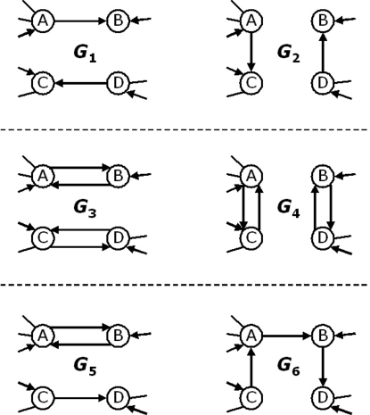
Figure 3: In the directed version of the configuration model, the local rewiring algorithm symmetry1 has various generalizations. If one requires that only the two degree sequences $\{k^{in}_{i}\}$ and $\{k^{out}_{i}\}$ are preserved, with $H(G)$ defined by Equation (58), then each graph on the left has the same probability of occurrence as the corresponding graph on the right, since $H(G_{1})=H(G_{2})$, $H(G_{3})=H(G_{4})$ and $H(G_{5})=H(G_{6})$. By additionally requiring that also $\{k^{\leftrightarrow}_{i}\}$ is preserved, and redefining $H(G)$ as in Equation (62), the above symmetry of the Hamiltonian is broken: $G_{5}$ and $G_{6}$ are no longer equiprobable since now $H(G_{5})\neq H(G_{6})$.

In this case the maximum likelihood principle mylikelihood indicates that, in order to provide a null model of a real network $G^{*}$, the parameters $\{x_{i}\}$, $\{y_{i}\}$ and $\{z_{i}\}$ must be set to the particular values $\{x^{*}_{i}\}$, $\{y^{*}_{i}\}$ and $\{z^{*}_{i}\}$ satisfying the $3N$ coupled equations

$$\langle k^{in}_{i}\rangle = \sum_{j\neq i}\frac{x^{*}_{i}y^{*}_{j}+x^{*}_{i}x^{*}_{j}y^{*}_{i}y^{*}_{j}z^{*}_{i}z^{*}_{j}}{1+x^{*}_{i}y^{*}_{j}+x^{*}_{j}y^{*}_{i}+x^{*}_{i}x^{*}_{j}y^{*}_{i}y^{*}_{j}z^{*}_{i}z^{*}_{j}}=k^{in}_{i}(G^{*})\qquad\forall i$$ (67)

$$\langle k^{out}_{i}\rangle = \sum_{j\neq i}\frac{x^{*}_{j}y^{*}_{i}+x^{*}_{i}x^{*}_{j}y^{*}_{i}y^{*}_{j}z^{*}_{i}z^{*}_{j}}{1+x^{*}_{i}y^{*}_{j}+x^{*}_{j}y^{*}_{i}+x^{*}_{i}x^{*}_{j}y^{*}_{i}y^{*}_{j}z^{*}_{i}z^{*}_{j}}=k^{out}_{i}(G^{*})\qquad\forall i$$ (68)

$$\langle k^{\leftrightarrow}_{i}\rangle = \sum_{j\neq i}\frac{x^{*}_{i}x^{*}_{j}y^{*}_{i}y^{*}_{j}z^{*}_{i}z^{*}_{j}}{1+x^{*}_{i}y^{*}_{j}+x^{*}_{j}y^{*}_{i}+x^{*}_{i}x^{*}_{j}y^{*}_{i}y^{*}_{j}z^{*}_{i}z^{*}_{j}}=k^{\leftrightarrow}_{i}(G^{*})\qquad\forall i$$ (69)

ensuring that the expectation values of the three degree sequences equal the empirical ones. Again, we see that in this model the transpose equiprobability symmetry only holds if the real network $G^{*}$ has $k^{in}_{i}(G^{*})=k^{out}_{i}(G^{*})$ $\forall i$. In such a case, from the above equations one finds $x^{*}_{i}=y^{*}_{i}$ $\forall i$ which also implies $p_{ij}=p_{ji}$ and $H(A)=H(A^{T})$ so that all the expected topological properties have inward/outward invariance. Otherwise, the symmetry does not hold. A particular case of the above model turns out to empirically describe the World Trade Web, as we discuss in the next section.

5 Symmetries, Symmetry Breaking and the Evolution of World Trade

We now present an important real-world application of the concepts introduced so far, i.e. the evolution of the international trade network. The World Trade Web (WTW in the following) is the global network of import/export trade relationships among all world countries serrano ; mywtw ; myalessandria ; myinterplay ; 5 ; giorgiowtw . We already encountered the WTW in Section 3.2 among the other networks reported in Table 1. In the WTW, a vertex represents one country and a directed link represents the existence (during the period considered, usually one year) of an export relationship from one country to another country. The WTW is in principle a weighted network, since trade intensities can be measured by their (highly heterogeneous) total monetary values aggregated over the period. Therefore the properties of the network can be measured on a weighted basis 5 ; giorgiowtw . However, here we will consider the WTW as a binary network, and only refer to its purely topological properties. As we will show, even this simple picture is extremely interesting and allows an informative study of the international trade system. In particular, we will study how the network has evolved in time starting from the year 1950, and how a joint analysis of the trends displayed by different topological properties inform us about the change in the underlying symmetries. If the WTW is regarded as an undirected graph, its structural properties are remarkably stable over time, and indicate that the network displays a clear invariance under transformations that preserve its degree sequence. On the other hand, when the directionality of trade is taken into account, the above symmetry is broken and the intensity of this symmetry breaking changes in time. A strong increase in reciprocity is observed, clearly evidencing that a major structural change started taking place from the late 1970’s onwards. The symmetry concepts developed in Reference symmetry1 and in the previous sections will be employed to suggest, or rule out, possible explanations for the observed evolution of the WTW. In particular, we identify as candidate explanations a strong embedding in economic space and a spatial symmetry breaking in the production system, which is known to have occurred starting from the late 1970’s 7 ; 8 and could therefore explain the simultaneous change in the reciprocity of the network. Surprisingly, other mechanisms such as the increase in the number of trade relationships, size effects and the formation of trade agreements are not enough in order to explain the observed evolution of the symmetry properties considered. This analysis highlights the importance of identifying the behaviour of complex systems under different types of symmetries, and of introducing suitable measures that succeed in distinguishing between the latter.

5.1 Undirected Symmetries

Various empirical results describing the topology of the WTW can be combined in order to have a detailed picture of the underlying symmetries. In this section we consider the undirected projection of the network as defined in Section 3.4, while in the next one we consider the WTW as a directed network. A first interesting observation, that will be useful in the following, is that the undirected connectance $\bar{b}$ defined by Equation (36) remains almost constant during the time interval considered, as shown in Figure 4. This happens despite the fact that the number $N(t)$ of world countries increases significantly, due to a number of new independent states being formed between 1948 and 2000.

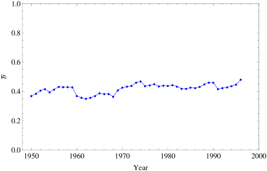
Figure 4: Evolution of the density $\bar{b}(t)$ of the undirected version of the World Trade Web.

Importantly, the constancy of the connectance does not mean that the latter characterises the WTW satisfactorily. If we use the random graph model as a null model of the WTW, the undirected connection probability defined in Equation (48) is uniform: $q_{ij}(t)=q(t)$. The maximum likelihood principle, in accordance with Equation (9), indicates the following choice for this probability:

$$q^{*}(t)=\frac{2L^{u}(t)}{N(t)[N(t)-1]}$$ (70)

However, the above choice generates trivial expectations which are not in accordance with the empirical results, in particular a Binomial degree distribution, a constant (uncorrelated with the degree) average nearest neighbour degree and a constant clustering coefficient. This means that the ensemble equiprobability invariance of the random graph model under transformations preserving the total number of links is not a stochastic symmetry of the WTW in the sense explained in Section 2.1.

By contrast, an important finding myrandomization ; mywtw is that, in every snapshot of the network within the time window considered, the undirected projection of the WTW is always remarkably well reproduced by the configuration model. This means that, according to Equation (11), the probability that a trade relationship exists (irrespective of its direction) between two countries $i$ and $j$ in a given year $t$ is

$$q_{ij}(t)=\frac{w^{*}_{i}(t)w^{*}_{j}(t)}{1+w^{*}_{i}(t)w^{*}_{j}(t)}$$ (71)

where the parameters $\{w^{*}_{i}(t)\}$ are the solution of the $N$ coupled equations

$$\langle k_{i}(t)\rangle=\sum_{j\neq i}\frac{w^{*}_{i}(t)w^{*}_{j}(t)}{1+w^{*}_{i}(t)w^{*}_{j}(t)}=k_{i}(t)\qquad\forall i$$ (72)

which are equivalent to Equation (12). The accordance between the configuration model and the real undirected WTW has been checked by studying various higher-order properties, including the average nearest neighbour degree and the clustering coefficient of all vertices, and confirming that they are excellently reproduced by the model myrandomization ; mywtw . The undirected WTW is therefore a good example of a network whose higher-order properties can be traced back to low-level constraints. According to our discussion in Section 2.1, this implies that the ensemble equiprobability invariance displayed by the configuration model under transformations preserving the degree sequence symmetry1 is a stochastic symmetry of the real WTW. In turn, this implies that in every snapshot of the WTW all vertices with the same degree $k$ are statistically equivalent symmetry1 . That is, the overall symmetry of the network under permutations of vertex labels is broken down to distinct universality classes consisting of vertices with the same degree. This is evident from the fact that, in passing from the random graph model (where all vertices are statistically equivalent) to the configuration model (where all vertices with the same degree are statistically equivalent), the connection probability changes from Equations (70) to (71) and therefore acquires a dependence on the variables $w_{i}^{*}$ and $w_{j}^{*}$, which in turn depend on the degree sequence through Equation (72). Unlike $q(t)$, the probability $q_{ij}(t)$ is not uniform across all pairs of vertices, but only across pairs of vertices with the same pair of degrees $k_{i}$ and $k_{j}$. As shown in Equation (51), the following relation holds between the expected connectance $\langle\bar{b}\rangle$ and the probability $q_{ij}(t)$:

$$\langle\bar{b}(t)\rangle=\frac{2\sum_{i<j}q_{ij}(t)}{N(N-1)}=\frac{2}{N(N-1)}\sum_{i<j}\frac{w^{*}_{i}(t)w^{*}_{j}(t)}{1+w^{*}_{i}(t)w^{*}_{j}(t)}$$ (73)

Therefore the observed stationarity of $\bar{b}$ shown in Figure 4 indicates that, despite $q_{ij}(t)$ varies greatly among pairs of world countries and also over time, its average across all pairs of countries remains remarkably stable.

The accordance between the undirected WTW and the configuration model means that the degree sequence is extremely informative, since its knowledge allows one to obtain correct expectations about all other topological properties. This implies that, in order to explain the WTW topology at an undirected level, it is enough to explain its degree sequence. Thus reproducing the degree sequence should be the target of any model of the WTW topology, an important point that we will discuss in Section 5.3. Whatever the cause of the empirical degree sequence of WTW, this cause is the symmetry-breaking phenomenon restricting the invariance of the network to degree-preserving transformations.

5.2 Directed Symmetries

We now come to the description of the WTW as a directed network, which involves additional information. Note that, since the configuration model reproduces the real WTW topology, and since in this model different pairs of vertices are statistically independent, then also the directed version of the model must be reproduced by a model with independent pairs of vertices. What remains to be clarified is whether the possible events that can occur within a single pair of vertices are also statistically independent, i.e. whether the conditional connection probability $r_{ij}$ and the marginal connection probability $p_{ij}$ defined in Section 3.4 are equal. In other words, we need to characterise the reciprocity structure of the network.

To this end, a first useful result is that, irrespective of the year $t$ considered, the in-degree and the out-degree of every vertex are empirically found to be approximately equal myreciprocity ; myalessandria ; myinterplay , i.e.

$$k^{in}_{i}(t)\approx k^{out}_{i}(t)\qquad\forall i$$ (74)

A second empirical result is that the reciprocated degree $k^{\leftrightarrow}_{i}(t)$ defined in Equation (27) is always proportional to the total degree $k^{tot}_{i}(t)=k^{in}_{i}(t)+k^{out}_{i}(t)$, with a time-dependent proportionality coefficient myreciprocity ; myalessandria :

$$k^{\leftrightarrow}_{i}(t)\propto k^{tot}_{i}(t)\qquad\forall i$$ (75)

This result is shown in Figure 5 for various years $t$.

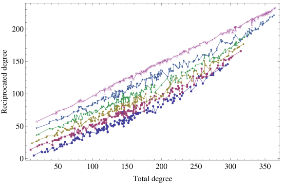
Figure 5: Dependence of the reciprocated degree $k^{\leftrightarrow}_{i}$ on the total degree $k^{tot}_{i}=k^{in}_{i}+k^{out}_{i}$ in various snapshots of the WTW (from bottom to top: $t=1975,1980,1985,1990,1995,2000$). The different curves have been shifted vertically for better visibility.

Taken together, these two results inform us about the structure of the connection probabilities $p_{ij}$, $r_{ij}$ and $p_{ij}^{\leftrightarrow}$ introduced in Section 3.4. Indeed, since $\langle k^{in}_{i}(t)\rangle=\sum_{j\neq i}p_{ji}(t)$ and $\langle k^{out}_{i}(t)\rangle=\sum_{j\neq i}p_{ij}(t)$, the result in Equation (74) can be rephrased as

$$p_{ij}(t)\approx p_{ji}(t)\qquad r_{ij}(t)\approx r_{ji}(t)$$ (76)

Similarly, since $\langle k^{\leftrightarrow}_{i}(t)\rangle=\sum_{j\neq i}r_{ij}(t)p_{ji}(t)$, Equation (75) implies that $r_{ij}(t)$ is independent of $i$ and $j$, i.e. the conditional connection probability is uniform:

$$r_{ij}(t)\approx r_{0}(t)$$ (77)

The latter determines the proportionality coefficient relating the reciprocated degree to the total degree as in Equation (75):

$$\langle k_{i}^{\leftrightarrow}(t)\rangle=r_{0}(t)\sum_{j\neq i}p_{ij}(t)=r_{0}(t)\langle k^{out}_{i}(t)\rangle=\frac{r_{0}(t)}{2}\langle k^{tot}_{i}(t)\rangle$$ (78)

Moreover, Equation (46) implies that the expected reciprocity of the network at time $t$ coincides with the conditional connection probability:

$$\langle r(t)\rangle\approx r_{0}(t)$$ (79)

This result can be confirmed independently,by measuring the observed reciprocity $r(t)$ and checking that it is indeed approximately equal to the proportionality coefficient $r_{0}(t)$ relating the reciprocated degree to the total degree as in Equation (78), obtained from a linear fit of the trends shown in Figure 5 myreciprocity . We will show more empirical results about the reciprocity in Section 5.4.

The uniformity of $r_{ij}(t)$ implies that the marginal connection probability must be different from the conditional one. Otherwise, the WTW would be well reproduced by the directed random graph model introduced in Section 4, with $p(t)\approx r_{0}(t)$. This possibility is ruled out by the fact that the two approximate equalities $p_{ij}(t)\approx p_{ji}(t)$ and $r_{ij}(t)\approx r_{0}(t)$, if inserted into Equation (48), imply

$$q_{ij}(t)\approx[2-r_{0}(t)]p_{ij}(t)$$ (80)

which, together with Equation (71), implies that the WTW is well described by the marginal connection probability

$$p_{ij}(t)\approx\frac{1}{2-r_{0}(t)}q_{ij}(t)=\frac{1}{2-r_{0}(t)}\frac{w^{*}_{i}(t)w^{*}_{j}(t)}{1+w^{*}_{i}(t)w^{*}_{j}(t)}$$ (81)

The above marginal probability is not uniform as the directed random graph model would predict, and is necessarily different from the uniform conditional connection probability $r_{0}(t)$. This means that the reciprocity of the WTW, whatever the snapshot considered, is nontrivial. As another consequence, this result implies that a good model of the WTW is not even provided by the directed configuration model defined by Equation (58), because the latter predicts $r_{ij}=p_{ij}$ as shown in Equation (59). Therefore the directed representation of the WTW does not display, as a stochastic symmetry, the ensemble equiprobability invariance under transformations that preserve the degree sequences $\{k^{in}_{i}\}$ and $\{k^{out}_{i}\}$.

As discussed in Section 4, a step forward the simple directed configuration model is provided by the model defined by Equation (62), i.e. a maximum-entropy ensemble of graphs with constraints given by the three degree sequences $\{k^{out}_{i}\}$, $\{k^{in}_{i}\}$, $\{k^{\leftrightarrow}_{i}\}$ controlled by the Lagrange multipliers $\{\theta^{out}_{i}\}$, $\{\theta^{in}_{i}\}$, $\{\theta^{\leftrightarrow}_{i}\}$ or equivalently $\{x_{i}\}$, $\{y_{i}\}$, $\{z_{i}\}$. We now prove various theoretical relations describing what is implied when a uniform conditional connection probability $r_{ij}=r_{0}$ is assumed as a further ingredient of this model, and show that these relations are in excellent agreement with all the empirical properties of the WTW discussed above, and reconcile the undirected picture with the directed one. For brevity, in our notation we drop the dependence of the various quantities on the time $t$. First, note that, due to the equality $p_{ij}r_{ji}=p_{ji}r_{ij}$ appearing for instance in Equation (39), $r_{ij}=r_{0}$ implies

$$p_{ij}=p_{ji}$$ (82)

and automatically predicts both $\langle k^{in}_{i}\rangle=\langle k^{out}_{i}\rangle$ and $\langle k^{\leftrightarrow}_{i}\rangle=(r_{0}/2)\langle k^{tot}_{i}\rangle$. In other words, the constancy of $r_{ij}$ implies the symmetry of $p_{ij}$ and is enough to simultaneously explain the two empirical properties of the WTW reported in Equations (74) and (75). As another consequence, one has $x_{i}=y_{i}$ $\forall i$ in Equation (65) so that Equation (66) becomes

$$r_{ij}=\frac{x_{i}x_{j}z_{i}z_{j}}{1+x_{i}x_{j}z_{i}z_{j}}$$ (83)

But under our hypothesis the above expression must be a constant $r_{0}$, which is only possible if $x_{i}z_{i}=y_{i}z_{i}=\alpha$ where $\alpha$ is a constant. This implies

$$x_{i}=y_{i}=\alpha z_{i}^{-1}\qquad\Leftrightarrow\qquad\theta^{out}_{i}=\theta^{in}_{i}=-\ln\alpha-\theta^{\leftrightarrow}_{i}$$ (84)

Therefore among the three parameters $x_{i}$, $y_{i}$, $z_{i}$ there is only an independent one (say $x_{i}$). This allows us to rewrite Equations (63) and (64) as

$$p^{\to}_{ij} = \frac{x_{i}x_{j}}{1+(2+\alpha^{2})x_{i}x_{j}}$$ (85)

$$p^{\leftrightarrow}_{ij} = \frac{\alpha^{2}x_{i}x_{j}}{1+(2+\alpha^{2})x_{i}x_{j}}$$ (86)

and Equations (65) and (66) as

$$p_{ij} = \frac{(1+\alpha^{2})x_{i}x_{j}}{1+(2+\alpha^{2})x_{i}x_{j}}$$ (87)

$$r_{ij} = r_{0}=\frac{\alpha^{2}}{1+\alpha^{2}}$$ (88)

The last equation, if inserted into Equation (46), implies

$$\langle r\rangle=r_{ij}=\frac{\alpha^{2}}{1+\alpha^{2}}$$ (89)

which clearly shows that in this model the expected reciprocity $r$ coincides with the conditional probability $r_{ij}$ and is uniquely determined by $\alpha$. Thus all the above quantities could be expressed as functions of $r_{0}$ (or $\langle r\rangle$) rather than $\alpha$, by exploiting the inverse relation

$$\alpha=\sqrt{\frac{r_{0}}{1-r_{0}}}=\sqrt{\frac{\langle r\rangle}{1-\langle r\rangle}}$$ (90)

Equation (48) implies that under the above model the connection probability in the undirected projection of the network is

$$q_{ij}=p_{ij}+p_{ji}-r_{ij}p_{ji}=\frac{(2+\alpha^{2})x_{i}x_{j}}{1+(2+\alpha^{2})x_{i}x_{j}}$$ (91)

Together with Equations (87) and (90), the above relation implies

$$q_{ij}=\frac{2+\alpha^{2}}{1+\alpha^{2}}p_{ij}=(2-r_{0})p_{ij}$$ (92)

which exactly reproduces the empirical property of the WTW shown in Equation (80). Note that, if the parameters $\alpha$ and $\{x_{i}\}$ are tuned to the values $\alpha^{*}$ and $\{x^{*}_{i}\}$ fitting the model to the real network, Equation (91) coincides with Equation (71) once $\alpha^{*}$ is reabsorbed into $w^{*}_{i}$ as follows:

$$w_{i}^{*}=x_{i}^{*}\sqrt{2+(\alpha^{*})^{2}}$$ (93)

That is, once the value of $\alpha^{*}$ enforcing the observed value of the reciprocity is fixed, the values of $\{x_{i}^{*}\}$ determine the undirected degree sequence exactly as $\{w_{i}^{*}\}$ in the undirected configuration model. This important result indicates that the undirected version of the directed model considered here coincides with the undirected configuration model, and thus reconciles the directed and undirected descriptions. Note that this is not true in general: for instance, the undirected version of the directed configuration model defined by Equation (58) does not coincide with the undirected configuration model. It is the nontrivial structure of the reciprocity of the WTW, manifest in the uniformity of $r_{ij}$, that ensures this property. This result can be confirmed by noticing that Equation (84) implies that the Hamiltonian of the model, which in general has the form in Equation (62), in this case becomes

$$H(G) = \sum_{i}[\theta_{i}k_{i}^{out}+\theta_{i}k_{i}^{in}+(\theta_{0}-\theta_{i})k_{i}^{\leftrightarrow}]$$ (94)

$$= \sum_{i}\theta_{i}k_{i}+\theta_{0}L^{\leftrightarrow}$$

where we have defined $\theta_{i}\equiv\theta_{i}^{in}=\theta_{i}^{out}=-\ln x_{i}$ and $\theta_{0}\equiv-\ln\alpha$. The above expression highlights that the constraints required in order to reproduce all the topological properties of the WTW discussed so far are the undirected degree sequence $\{k_{i}\}$ and the number of reciprocated links $L^{\leftrightarrow}$, or equivalently the reciprocity $r$. If the maximum likelihood principle mylikelihood is applied to this model, it is straightforward to show that the parameters reproducing a given snapshot of the WTW must be set to the particular values $\alpha^{*}=e^{-\theta_{0}^{*}}$ and $\{x^{*}_{i}\}=\{e^{-\theta^{*}_{i}}\}$ satisfying the following $N+1$ coupled equations

$$\langle k_{i}\rangle = \sum_{j\neq i}q_{ij}=\sum_{j\neq i}\frac{[2+(\alpha^{*})^{2}]x^{*}_{i}x^{*}_{j}}{1+[2+(\alpha^{*})^{2}]x^{*}_{i}x^{*}_{j}}=k_{i}\qquad\forall i$$ (95)

$$\langle L^{\leftrightarrow}\rangle = \sum_{i\neq j}r_{ji}p_{ij}=\sum_{j\neq i}\frac{(\alpha^{*})^{2}x^{*}_{i}x^{*}_{j}}{1+[2+(\alpha^{*})^{2}]x^{*}_{i}x^{*}_{j}}=L^{\leftrightarrow}$$ (96)

The first of the two expressions above indeed coincides with the condition fixing the values of $\{w_{i}\}$ in the undirected configuration model as in Equation (72), under the identification given by Equation (93). The second expression allows to enforce any value of the reciprocity $r$ as additional constraint, thanks to the extra parameter $\alpha=e^{-\theta_{0}}$. Note that this graph ensemble is stochastically symmetric under link reversal, since $H(A)=H(A^{T})$. Furthermore, since the real WTW is well reproduced by the aforementioned graph ensemble, it is also stochastically symmetric under link reversal.

We have therefore shown that the topology of the WTW for any year $t$ since 1950 is completely reproduced by specifying the undirected degree sequence $\{k_{i}(t)\}$ and the reciprocity $r(t)$. This implies that, in order to explain why the WTW displays the structure we observe, it is enough to explain these two topological properties. However, while assessing the relevance of some structural features is a rigorous procedure as we have shown so far, explaining them in terms of underlying mechanisms involves a higher degree of uncertainty and subjective interpretation. Bearing this in mind, in what follows we suggest possible explanations for the two structurally informative ingredients of the WTW topology. These should be intended as candidate hypotheses rather than certain mechanisms. Nonetheless, since the symmetry of the effect must be at least that of the cause, the symmetry analysis carried out in the preceding sections can be exploited to safely rule out explanations that do not fulfill this principle.

5.3 Topological Space and Embedding Spaces

We start by considering here the undirected degree sequence, while in the next section we focus on the reciprocity. The accordance between the configuration model and the undirected projection of the WTW, i.e. the stochastic symmetry of the WTW under transformations preserving the degree sequence, can be rephrased as the finding that the network is the result of a random matching process between the edges attached to every vertex. Vertices connect to each other as the mere result of the constraint on their degrees. The larger their degrees, the higher the probability that two vertices are connected, with no higher-order effect on the topology. This implies that, whatever the factor responsible for the observed degree of a country, it must similarly respect the symmetry and be such that the more a country is endowed with this factor, the larger its degree and the higher its probability to connect to other vertices, with no higher-order effect on the topology other than those implied by the degree sequence. If we denote the hidden factor as $h$, and its value for vertex $i$ as $h_{i}$, the above statement can be rephrased as the larger $h_{i}$, the larger the expected value of $\langle k_{i}\rangle$; similarly, the larger $h_{i}$ and $h_{j}$, the larger the undirected connection probability $q_{ij}$. Therefore the hidden values $\{h_{i}\}$ must play exactly the same role as that of the Lagrange multipliers $\{w_{i}\}$ controlling the expected degrees of all vertices in the undirected configuration model as in Equation (72). More in general, the Lagrange multiplier $w_{i}$ could be a monotonic function $f(h_{i})$ of the hidden factor $h_{i}$. The above consideration suggests at least two ways to test whether any empirically observable quantity is indeed a good candidate as the hidden factor determining the degree sequence in a given snapshot of the WTW. First, one can solve the $N$ coupled equations in Equation (72) and obtain the set of values $\{w_{i}^{*}(t)\}$ which are the exact values of the Lagrange multipliers enforcing the observed degree sequence in year $t$, and then check whether a candidate quantity $h(t)$, with empirically observed values $\{h_{i}(t)\}$, is indeed in some approximate functional dependence with these multipliers, i.e.

$$w^{*}_{i}(t)\approx f[h_{i}(t),h_{0}(t)]\quad\forall i$$ (97)

where $f$ can in general depend on, besides $h_{i}(t)$, a global time-dependent parameter $h_{0}(t)$ setting the scale of the dependence. As a second alternative, one could assume the functional dependence $w_{i}(t)=f[h_{i}(t),h_{0}(t)]$, rewrite $q_{ij}(t)$ as

$$q_{ij}(t)=\frac{w_{i}(t)w_{j}(t)}{1+w_{i}(t)w_{j}(t)}=\frac{f[h_{i}(t),h_{0}(t)]f[h_{j}(t),h_{0}(t)]}{1+f[h_{i}(t),h_{0}(t)]f[h_{j}(t),h_{0}(t)]}$$ (98)

and apply the maximum likelihood principle to the resulting model, which now has only $h_{0}(t)$ as a free parameter since the values $\{h_{i}(t)\}$ are empirically accessible. This leads to the single equation

$$\langle L^{u}(t)\rangle=\sum_{i<j}\frac{f[h_{i}(t),h^{*}_{0}(t)]f[h_{j}(t),h^{*}_{0}(t)]}{1+f[h_{i}(t),h^{*}_{0}(t)]f[h_{j}(t),h^{*}_{0}(t)]}=L^{u}(t)\quad\forall i$$ (99)

fixing the value of $h_{0}(t)$ for each year $t$ and replacing Equation (72). The goodness of the assumed dependence can be tested by checking whether Equation (98), with the value $h^{*}_{0}(t)$ inserted in it, reproduces the properties of the real network, in the same way as Equation (72) is used to assess the goodness of the configuration model. Clearly, the first procedure is preferable as it leaves the determination of the form of $f[h_{i}(t),h_{0}(t)]$ at the end: once the values $\{w_{i}^{*}(t)\}$ are found exactly, one can study the dependence of the latter on various candidate quantities $h$, and with different functional forms. The second procedure requires from the beginning the assumption one wants to test, and is therefore less accurate; nonetheless, it could represent a further test of the hypothesis if the output of the first method is used as the input in the second one.

Both the approaches described above have been used to look for hidden factors explaining the degree sequence, and consequently the entire topology, of the undirected WTW mylikelihood ; mywtw . The result of this analysis is that the Gross Domestic Product (GDP in what follows) is a very good candidate factor. If $h_{i}(t)$ is identified with the empirical GDP value of country $i$ in year $t$, then an approximate linear relationship between $h_{i}(t)$ and the value $w_{i}^{*}(t)$ obtained from Equation (72) for the same year is observed mylikelihood . This means that Equation (97) reduces to the simplest possible functional form

$$w^{*}_{i}(t)\approx h_{i}(t)\sqrt{h_{0}(t)}\quad\forall i$$ (100)

where the proportionality factor has been denoted as $\sqrt{h_{0}(t)}$ for convenience. This indicates that the probability that a trade relationship (whatever its direction) exists between countries $i$ and $j$ in year $t$ is

$$q_{ij}(t)\approx\frac{h_{0}(t)h_{i}(t)h_{j}(t)}{1+h_{0}(t)h_{i}(t)h_{j}(t)}$$ (101)

This result is confirmed by assuming the above form of the connection probability, using Equation (99) to find the value $h^{*}_{0}(t)$ generating the observed number of links, and checking that indeed the empirical properties of the undirected WTW are reproduced mywtw . This result highlights that the larger (in economic terms) a country, the higher its probability to connect to other countries. According to our discussion at the end of Section 5.1, since the GDP is responsible for the degree sequence of the WTW, it represents the symmetry-breaking variable restricting the invariance of the network to equal-degree (or similarly equal-GDP) equivalence classes. Contrary to what one could expect on the basis of the spatial embedding of the WTW, no significant dependence is found on other factors such as distance, membership to common geographic areas or trade associations, etc.

The above result is very instructive in the light of the relation between network structure and symmetry. What we should bear in mind, when we consider symmetry breaking in the field of network theory, is that symmetry (invariance) is hard to depict unless we use analytical tools. Our imagination, intended as the faculty of forming images, has been educated to depict shapes in Euclidean spaces. Whenever we must traduce shapes from Euclidean to topological spaces, we are inevitably biased by the fact the we tend to recall the Euclidean representation of forms in the new space. This overlapping of spaces generates misrepresentation. To better stress out the conundrum of spaces’ inequality representation, in Figure 6 we picture the trade network of Europe (EU-15), as it would appear in topological space (left panel) and in Euclidean space (middle panel), assuming that trades travel mainly on the road network road . While the Euclidean representation of the road network, except for the scale and a certain degree of abstraction, is conformal to the real system’s shape, the corresponding representation of the trade network in a metric space (the plane), is purely conventional. Indeed, we could have represented the same network in several different ways, e.g., arraying in a circle or randomly scattering nodes. We could actually produce ad libitum different Euclidean embeddings of the same graph. The topological-Euclidean dichotomy is further complicated by the fact the system represented by the WTW network is immersed in an economic space, involving variables and relations in large number, that are not detected in the network. Consider for example the traveling time of goods, which is determined by several exogenous factors. Traveling time, together with energy efficiency and labor costs, is among the major factors affecting shipping costs. In the right panel of Figure 6 we show a ‘metric representation’ of the space modification due to traveling time times . It is noteworthy that in an economic space distances are not merely Euclidean and the compound metric is made by length, time, labor costs and energy units at the minimum.

Indeed, the result that the WTW is excellently reproduced by a connection probability that uniquely depends on the GDP indicates that the space modification is even more extreme, as at a global level geographic distances appear to play almost no role. In regular lattices the overall permutation symmetry of vertices is broken by positions in Euclidean space and is restricted to invariances of lesser order such as translational symmetry symmetry1 . In geographically embedded networks such as that shown in the middle panel of Figure 6, the irregularity of the geography further restricts the symmetry properties. When additional variables are also taken into account, even stronger distortions take place as in the right panel of Figure 6, and in the case of the WTW we are in an extreme situation where the symmetry-breaking variable is virtually only the GDP, and the distance dependence practically disappears. The properties of the network must be therefore interpreted in economic space rather than geographic space. Still, in this space we find a remarkable symmetry: countries with the same GDP are statistically equivalent symmetry1 , and pairs of countries with the same couple of GDP values have the same probability to trade. In other words, we can rephrase the symmetry properties of the WTW we discussed in Section 5.1 in terms of the GDP values rather than the degree sequence. This invariance is preserved despite the heterogeneity of the GDP across world countries increases in time myinterplay , which means that the intensity of the GDP-induced symmetry breaking also increases. And, despite the latter determines ever-increasing divergences between the values of the connection probability $q_{ij}$ across pairs of countries, the average probability $2\sum_{i<j}q_{ij}/N(N-1)$ remains almost constant as indicated by the stationarity of the undirected connectance shown in Figure 4.

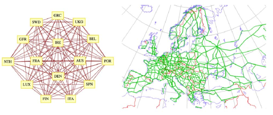
Figure 6: European (EU-15) trade network as it would appear in topological space (left panel), in Euclidean space assuming that trades travel mainly on the road network (middle panel, after road ), and after also taking into account the space modification due to traveling times (right panel, after times ).

5.4 The Reciprocation Process of World Trade and Spatial Symmetry Breaking

As we mentioned, the second ingredient required in order to explain the topological properties of the WTW is the reciprocity $r$, which coincides with the conditional connection probability $r_{0}$ as indicated by Equation (79). While we have shown that the marginal connection probability varies greatly among different pairs of vertices, a property that can be traced back to the heterogeneous degrees and possibly explained by the GDP values, the conditional connection probability is uniform and must therefore be related to a completely different mechanism. The heterogeneity of vertex degrees, or of GDP values, is completely reflected in the marginal connection probability while it is not reflected at all in the conditional connection probability and in the reciprocity. To better understand the problem, we now consider the temporal evolution of the reciprocity and show how this may suggest possible explanations.

As clear from Equations (75) and (78), the proportionality constant $r_{0}(t)/2$ between $k^{\leftrightarrow}_{i}(t)$ and $k^{tot}_{i}(t)$ is time-dependent. As Equation (79) indicates, this means that the reciprocity $r(t)=r_{0}(t)$ of the network must also change in time. In Figure 7 we show the empirical evolution of $r(t)$. Indeed, we find that the reciprocity of the WTW has evolved dramatically during the period considered. In particular, we see that $r(t)$ has been fluctuating about a constant value from 1950 to the late 1970’s. Then, from the late 1970’s to the late 1990’s, a steady increase of $r(t)$ took place. More importantly, this occurred despite the density of undirected trade relationships (the undirected connectance $\bar{b}$ shown in Figure 4) remained approximately constant during the same period. This indicates that, from the late 1970’s on, there has been an establishment of many new directed trade relationships mainly between countries that had already been trading in the opposite direction, rather than between countries that had not been trading at all. That is, the reciprocation process of unidirectional trade channels has dominated the formation of new trade relationships between non-interacting countries.

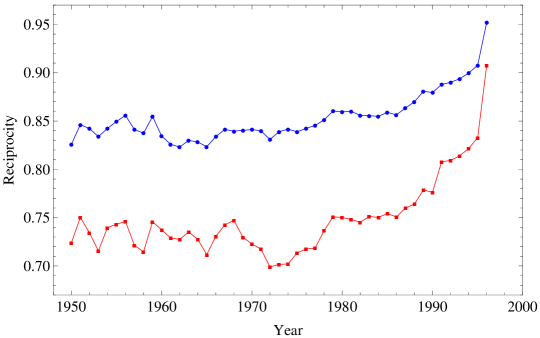
Figure 7: Evolution of the reciprocity measures $r(t)$ (blue points) and $\rho(t)$ (red points) in the directed version of the World Trade Web.

The above results have implications for the evolution of the symmetry properties of the network. As it was highlighted in the previous sections, the equiprobability symmetry of the configuration model allows a statistical interpretation of the real undirected WTW. Higher order topological variables can be explained by the degree sequence. The invariance of the Hamiltonian is preserved through time, as reflected by the stationarity of some topological variables (Figure 4). The stationarity is however disrupted as we change lens and move from the undirected to the directed graph. Reciprocity determines a clear symmetry breaking in the directed analogue of the above invariance, as the in- and out-degrees alone are no longer enough to characterise the network. The intensity of this symmetry breaking evolves in time, as evident in the trend of the reciprocity $r(t)$, and even more of $\rho(t)$. Also, while the second type of link reversal symmetry (transpose equiprobability) is approximately unchanged over time, since the approximate equality $k^{in}_{i}(t)\approx k^{out}_{i}(t)$ holds throughout the interval considered, the adjacency matrix suddenly starts becoming more symmetric: $A$ and $A^{T}$ become more and more similar in time, indicating that the WTW has undergone a strong evolution towards higher levels of link reversal symmetry of the first type (transpose equivalence). The reason of such a sudden change is obscure. The evolution may have been either driven by other topological variables, i.e. it was endogenous to the network, or determined by some hidden variables, thus exogenous to the network. In other words: the change either pertains thoroughly the topological space or comes from an ‘outer embedding space’, where the exogenous variables belong to, that shapes the topological space symmetry1 . Besides, it may also be possible that the symmetry breaking actually occurred in this latter space and consequently affected the topological space. In what follows we explore this problem in more detail.

A first natural explanation of the above empirical result could be looked for in an overall increase in the number of directed trade relationships during the period considered, a possibility consistent with the globalisation process. Note that in our case Equation (36) implies that, while the undirected connectance $\bar{b}(t)$ is approximately constant, the directed connectance $\bar{a}(t)$ (hence the density of directed trade relationships) of the WTW has indeed increased significantly due to the observed increase of $r(t)$. In order to understand whether the observed increase in reciprocity is merely due to the overall increase in link density, it is important to recall our discussion in Section 3.2, where we stressed the importance of using $\rho$ instead of $r$ since the former washes away density effects. Since in this case the link density $\bar{a}(t)$ changes in time, using $\rho(t)$ instead of $r(t)$ is also important in order to correctly quantify the temporal evolution of the reciprocity. In Figure 7, besides $r(t)$, we also show the evolution of $\rho(t)$. Unlike $r(t)$, the behaviour of $\rho(t)$ is informative and clearly shows that the increase in density cannot explain the increase in reciprocity. Remarkably, the evolution of $\rho(t)$ is even more pronounced than that of $r(t)$, indicating that the change in density determines an underestimation of the steep increase in reciprocity, if the latter is measured by $r$ rather than by $\rho$. The same consideration applies even if one takes into account the fact that, according to our results discussed above, the increase in the density of directed trade relationships has occurred differentially across world countries, i.e. not uniformly as in a directed random graph model with increasing connection probability $p(t)$ but rather as in a directed configuration model with heterogeneous probabilities $p_{ij}(t)$. If the observed increase in reciprocity were merely due to a differential, rather than homogeneous, increase of link density, then we would observe $r_{ij}\approx p_{ij}$ as discussed in Section 5.2. By contrast, the uniformity of $r$ rules out this possibility. In other words, the inadequacy of the random graph model and the configuration model in reproducing the observed properties of the WTW rules out the possibility that the increase in reciprocity is due to the globalisation process, at least the component of the latter that is responsible for an (either homogeneous or differential) increase in the density of directed trade relationships.

As a second hypothesis, one could consider the establishment of new trade agreements (preferentially between countries that had only unidirectional trade relationships, and determining the reciprocation of the latter) as a possible explanation for the increase in the density of reciprocated links. However, trade agreements do not explain the uniformity of the conditional connection probability $r_{ij}(t)=r_{0}(t)$. For all years, the latter is empirically found to be the same across all pairs of vertices, which is in contrast with what expected from the formation of trade agreements: an increased value of $r_{ij}(t)$ for pairs of countries signing the agreement, determining an increased heterogeneity of $r_{ij}(t)$ across all pairs. Therefore the evolution in $r$ cannot be explained by the formation of trade agreements. The uniformity of the conditional connection probability also indicates that other factors such as size, distance, etc. appear to be not enough in order to explain how the reciprocity of world trade has evolved.

The above considerations show that the reciprocation of preexisting unidirectional relationships appears to have occurred massively, however with no preference for nearby or richer countries, and in a way which cannot be traced back to an overall increase in the number of trade relationships and trade agreements. We stress again that all these factors must have had an impact on international trade patterns, especially on the intensity of trade relationships, however at a purely topological level they appear to be dominated by a different mechanism, which is uniform across all pairs of countries. In simplified terms, the evolution of the reciprocity of the WTW could be approximated by a process where, with time-varying but country-independent probability, a unidirectional trade relationship existing at time $t$ becomes reciprocated in the following year. Among the possible underlying mechanisms that could generate this process, we must look for one displaying a temporal trend which is synchronous with the one followed by the reciprocity of the WTW and shown in Figure 7. To this end, it is useful to recall that in the case of the WTW, vertices and links are samples of vertices and links of a larger underlying network. Indeed, countries themselves do not trade; rather, firms and consumers trade. Hence there are at least two submerged, and much larger, networks: one of goods—final products—and one of production factors—raw materials and semi-products (together with a third network related to the service market). The WTW may be considered as an overlapping map of these two networks. While the two hypotheses advanced above mainly concerned the network of final products, one could look for an explanation relative to the production network (a network composed by factories as vertices and productive means as links). The hypothesis that symmetry breaking occurred in the economic space of the industrial sector in a period starting between the 1970’s to the early 1980’s, with a significant worldwide impact on the productive structure, has been recently advanced 7 ; 8 . This transition was due on one hand to decreasing energy costs of transport means and on the other hand to raising labor costs. Firms therefore were stimulated to provide production factors outside the division and began dispersing the productive chain outside the company boundaries, sometimes abroad. This process, named by economists outsourcing, transformed the space of firms from a Euclidean space, where providers where separated from the production plant by physical distances, to an economic space where physical distances were secondary to other variables (i.e., changed the metric of economic space) 8 . This process was further reinforced by specialization and technological enhancement, and was one of the driving forces of globalisation. Note that, when a firm extends its productive chain outside the national boundaries, new links may appear in the trade network. This process can determine an increase in reciprocity, if the new countries entering the production process already import from the firm’s country. This mechanism can therefore provide a candidate explanation, from the production side of network flows, for the observed increase in reciprocity, which is also temporally consistent with the empirical trend. If this hypothesis, which must be further investigated, is correct, we would have faced a symmetry breaking in economic space affecting topological space, partially determining the phase transition we observe, and at the correct moment in time.

6 Conclusions

In this paper we took full advantage of our investigation of the symmetry properties of real networks symmetry1 to perform a detailed study in a specific case. We exploited our concept of stochastic graph symmetries to introduce a new definition of link reversal symmetry, i.e. transpose equiprobability. We showed that, when combined with other symmetry properties of directed networks, stochastic link reversal symmetry allows an improved understanding of the reciprocity of real networks. In particular, we have studied various symmetry properties of the World Trade Web across its evolution. Our analysis also sheds a light in a specific case on the symmetry properties of networks and symmetry breaking in network topology. We found that a space-symmetry approach to network theory may provide new insights into the complex structure of the underlying system. We also made a conjecture about the interplay between different spaces embedding the system, captured by the topological space, that may lie behind some dramatic changes observed in the detected topological variables. We believe that spatial symmetry breaking deserves more attention as it may lead to new perspectives in understanding complexity evolution and specifically, those kind of transformations characterized by a sudden leap in the complexity of the structure. Network theory represents a theoretical framework that enables holistic analyses and is suited to detect ongoing dynamics between the system’s components and the surrounding environment. In other words, network theory is a paradigm that considers the system as a whole and distributes its functioning in space and time. The analysis of the resulting symmetries carries information about the system.

More then twenty years ago, Marshall McLuhan, in the field of communication theory, advocated the need to overcome the constrains of conventional theories about communication, according to him relegated to an Euclidean and ‘visual’ space, to achieve a new theory based on an ubiquitous and synchronous space, in his words: an ‘acoustic space’. He advanced the point that space (and not just time) is an agent of communication. According to him, printed texts have educated us to a sequential type of communication, whereas the electronic age developed spatial communication: actors communicate in the same time with the environment and mutually between them 9 . Nevertheless, in his opinion, communication theory did not follow changes in communication media. In his own words: ‘The basis of all contemporary Western theories of communication—the Shannon-Weaver model—is a characteristic example of left-hemisphere lineal bias. It ignores the surrounding environment as a kind of pipeline model of a hardware container for software content. It stresses the idea of inside and outside and assumes that communication is a literal matching rather than making’ 10 .

We believe network theory is a paradigm intrinsically ‘spatial’ and ‘global’, that best suits the need for a holistic theory versus a sequential theory, that it could further benefit from the interaction with other disciplines and concepts. We considered here the case of symmetry and symmetry breaking, and showed that a formalisation of the relation between these phenomena and network properties is intriguing and informative, but at present still incomplete. One of the present limitations is due to the fact that the studied network is often a mere map of a larger, underlying network, embedded in Euclidean or non-Euclidean spaces. Symmetry breaking may occur in a different space, that is only indirectly represented in the topological space. This indirect consequence complicates a clear understanding of the underlying process, but stochastic symmetries appear to capture patterns that are unaccessible to exact symmetries. Future research must explore this scenario more thoroughly, and possibly shed light on the relation between network dynamics, symmetry breaking, the causal chain and its premises.

References

- (1) Garlaschelli, D.; Ruzzenenti, F.; Basosi, R. Complex networks and symmetry I: A review. Symmetry 2010, 2, X-X.
- (2) Rosen, J. Symmetry Discovered. Concepts and Applications in Nature and Science; Cambridge University Press: Cambridge, UK, 1975.
- (3) Lin, S.K. The Nature of the Chemical Process. 1. Symmetry Evolution —Revised Information Theory, Similarity Principle and Ugly Symmetry. Int. J. Mol. Sci. 2001, 2, 10–39.
- (4) Prigogine, Y. Time, Structure and Fluctuations; Nobel Lecture, 1977. http://nobelprize.org/nobel_prizes/chemistry/laureates/1977/prigogine–lecture.pdf
- (5) Mainzer, K. Symmetry and Complexity: The Spirit and Beauty of Nonlinear Science; World Scientific Publishing: Singapore, 2005.
- (6) Caldarelli, G. Scale-Free Networks: Complex Webs in Nature and Technology; Oxford University Press: Oxford, UK, 2007.
- (7) Caldarelli, G.; Vespignani, A. Large Scale Structure and Dynamics of Complex Networks; World Scientific Press: Singapore, 2007.
- (8) Barrat, A.; Barthelemy, M.; Vespignani, A. Dynamical Processes on Complex Networks; Cambridge University Press: New York, NY, USA, 2008.
- (9) Pascual, M.; Dunne, J.A. Ecological Networks: Linking Structure to Dynamics in Food Webs; Oxford University Press: New York, NY, USA, 2006.
- (10) Pastor-Satorras, R.; Vespignani, A. Evolution and Structure of the Internet: A Statistical Physics Approach; Cambridge University Press: Cambridge, UK, 2004.
- (11) Buchanan, M.; Caldarelli, G.; De Los Rios, P.; Rao, F.; Vendruscolo, M. Networks in Cell Biology; Cambridge University Press: UK, 2010.
- (12) Gross, T.; Sayama, H. Adaptive Networks; Springer/NECSI: Cambridge, Massachusetts (USA), 2009.
- (13) West, G.B.; Brown, J.H.; Enquist, B.J. The fourth dimension of life: fractal geometry and allometric scaling of organisms. Science 1999, 284, 1677–1679.
- (14) Banavar, J.R., Maritan, A.; Rinaldo, A. Size and form in efficient transportation networks. Nature 1999 399, 130–132.
- (15) Ruzzenenti, F.; Basosi, R. The rebound effect: An evolutionary perspective. Ecol. Econ. 2008, 67, 526–537.
- (16) Ruzzenenti, F.; Basosi, R. Complexity change and space symmetry rupture. Ecol. Model. 2009, 220, 1880–1885.
- (17) Garlaschelli, D.; Loffredo, M.I. Maximum likelihood: Extracting unbiased information from complex networks. Phys. Rev. E 2008, 78, 015101.
- (18) MacArthur, B.D.; Sánchez-García, R.J.; Anderson, J.W. Symmetry in complex networks. Discrete Appl. Math. 2008, 156, 3525–3531.
- (19) Xiao, Y.; MacArthur, B.D.; Wang, H.; Xiong, M.; Wang, W. Network quotients: Structural skeletons of complex systems. Phys. Rev. E 2008, 78, 046102.
- (20) MacArthur, B.D.; Sánchez-García, R.J. Spectral characteristics of network redundancy. Phys. Rev. E 2009, 80, 026117.
- (21) Wang, H.; Yan, G.; Xiao, Y. Symmetry in world trade network. J. Syst. Sci. Complex. 2009, 22, 280–290.
- (22) Squartini, T.; Garlaschelli, D. Exact maximum-likelihood method to detect patterns in real networks. Preprint available at http://arxiv.org/
- (23) Wasserman, S.; Faust, K. Social Network Analysis: Methods and Applications; Cambridge University Press: New York, NY, USA, 1994.
- (24) Garlaschelli, D.; Loffredo, M.I. Patterns of link reciprocity in directed networks. Phys. Rev. Lett. 2004, 93, 268701.
- (25) Garlaschelli, D.; Loffredo, M.I. Multispecies grand-canonical models for networks with reciprocity. Phys. Rev. E 2006, 73, 015101.
- (26) Meyers, L.A.; Newman, M.E.J.; Pourbohloul, B. Predicting epidemics on directed contact networks. J. Theor. Biol. 2006, 240, 400–418.
- (27) Boguna, M.; Serrano, M.A. Generalized percolation in random directed networks. Phys. Rev. E 2005, 72, 016106.
- (28) Perra, N.; Zlatic, V.; Chessa, A.; Conti, C.; Donato, D.; Caldarelli, G. PageRank equation and localization in the WWW. Europhys. Lett. 2009, 88, 48002.
- (29) Zamora-Lopez, G.; Zlatic V.; Zhou, C.; Stefancic, H.; Kurths, J. Reciprocity of networks with degree correlations and arbitrary degree sequences. Phys. Rev. E 2008, 77, 016106.
- (30) Zlatic V.; Stefancic, H. Influence of reciprocal edges on degree distribution and degree correlations. Phys. Rev. E 2009, 80, 016117.
- (31) Serrano, M.A.; Boguna, M. Topology of the world trade web. Phys. Rev. E 2003, 68, 015101.
- (32) Garlaschelli, D.; Loffredo, M.I. Fitness-Dependent Topological Properties of the World Trade Web. Phys. Rev. Lett. 2004, 93, 188701.
- (33) Garlaschelli, D.; Loffredo, M.I. Structure and evolution of the world trade network. Physica A 2005, 355, 138–144.
- (34) Garlaschelli, D.; Di Matteo, T.; Aste, T.; Caldarelli, G.; Loffredo, M.I. Interplay between topology and dynamics in the World Trade Web. Eur. Phys. J. B 2007, 57, 159–164.
- (35) Serrano, M.A. Phase transition in the globalization of trade. J. Stat. Mech. Theory Exp. 2007, Volume: 2007, L01002.
- (36) Fagiolo, G.; Reyes, J.; Schiavo S. World-trade web: Topological properties, dynamics, and evolution. Phys. Rev. E 2009, 79, 036115.
- (37) International E Road Network, http://en.wikipedia.org/wiki/File:International_E_Road_Network.png
- (38) Spiekermann, K.; Wegener, M. Trans-European Networks and Unequal Accessibility in Europe. Eur. J. Reg. Dev. (EUREG) 1996, 4, 35–42.
- (39) Richard, C. McLuhan and spatial communication. West. J. Commun. 2009, 63, 348–363.
- (40) McLuhan, M.; Powers, B. The Global Village: Transformations in World Life and Media in the 21st Century; New York: Oxford, UK, 1989.