Gravastars and Black Holes of Anisotropic Dark Energy

Abstract

Dynamical models of prototype gravastars made of anisotropic dark energy are constructed, in which an infinitely thin spherical shell of a perfect fluid with the equation of state $p=(1-\gamma)\sigma$ divides the whole spacetime into two regions, the internal region filled with a dark energy fluid, and the external Schwarzschild region. The models represent ”bounded excursion” stable gravastars, where the thin shell is oscillating between two finite radii, while in other cases they collapse until the formation of black holes. Here we show, for the first time in the literature, a model of gravastar and formation of black hole with both interior and thin shell constituted exclusively of dark energy. Besides, the sign of the parameter of anisotropy ($p_{t}-p_{r}$) seems to be relevant to the gravastar formation. The formation is favored when the tangential pressure is greater than the radial pressure, at least in the neighborhood of the isotropic case ($\omega=-1$).

I Introduction

Gravastar was proposed as an alternative to black holes. The pioneer of Mazur and Mottola (MM) MM01 , consists of five layers: an internal core $0<r<r_{1}$ , described by the de Sitter universe, an intermediate thin layer of stiff fluid $r_{1}<r<r_{2}$ , an external region $r>r_{2}$ , described by the Schwarzschild solution, and two infinitely thin shells, appearing, respectively, on the hypersurfaces $r=r_{1}$ and $r=r_{2}$. The intermediate layer is constructed in such way that $r_{1}$ is inner than the de Sitter horizon, while $r_{2}$ is outer than the Schwarzschild horizon, eliminating the apparent horizon. Configurations with a de Sitter interior have long history which we can find, for example, in the work of Dymnikova and Galaktionov irina . After this work, Visser and Wiltshire VW04 pointed out that there are two different types of stable gravastars which are stable gravastars and ”bounded excursion” gravastars. In the spherically symmetric case, the motion of the surface of the gravastar can be written in the form VW04 ,

$$\frac{1}{2}\dot{R}^{2}+V(R)=0,$$ (1)

where $R$ denotes the radius of the star, and $\dot{R}\equiv dR/d\tau$, with $\tau$ being the proper time of the surface. Depending on the properties of the potential $V(R)$, the two kinds of gravastars are defined as follows.

Stable gravastars: In this case, there must exist a radius $a_{0}$ such that

$$V\left(R_{0}\right)=0,\;\;\;V^{\prime}\left(R_{0}\right)=0,\;\;\;V^{\prime\prime}\left(R_{0}\right)>0,$$ (2)

where a prime denotes the ordinary differentiation with respect to the indicated argument. If and only if there exists such a radius $R_{0}$ for which the above conditions are satisfied, the model is said to be stable. Among other things, VW found that there are many equations of state for which the gravastar configurations are stable, while others are not VW04 . Carter studied the same problem and found new equations of state for which the gravastars are stable Carter05 , while De Benedictis et al DeB06 and Chirenti and Rezzolla CR07 investigated the stability of the original model of Mazur and Mottola against axial-perturbations, and found that gravastars are stable to these perturbations too. Chirenti and Rezzolla also showed that their quasi-normal modes differ from those of black holes with the same mass, and thus can be used to discern a gravastar from a black hole.

”Bounded excursion” gravastars: As VW noticed, there is a less stringent notion of stability, the so-called ”bounded excursion” models, in which there exist two radii $a_{1}$ and $a_{2}$ such that

$$V\left(R_{1}\right)=0,\;\;\;V^{\prime}\left(R_{1}\right)\leq 0,\;\;\;V\left(R_{2}\right)=0,\;\;\;V^{\prime}\left(R_{2}\right)\geq 0,$$ (3)

with $V(R)<0$ for $R\in\left(R_{1},R_{2}\right)$, where $R_{2}>R_{1}$.

Lately, we studied both types of gravastars JCAP -JCAP4 , and found that, such configurations can indeed be constructed, although the region for the formation of them is very small in comparison to that of black holes.

Based on the discussions about the gravastar picture some authors have proposed alternative models Chan . Among them, we can find a Chaplygin dark star Paramos , a gravastar supported by non-linear electrodynamics Lobo07 , a gravastar with continuous anisotropic pressure CattoenVisser05 and recently, Dzhunushaliev et al. worked on spherically symmetric configurations of a phantom scalar field and they found something like a gravastar but it was unstablesingleton . In addition, Lobo Lobo studied two models for a dark energy fluid. One of them describes a homogeneous energy density and the other one describes an ad-hoc monotonically decreasing energy density, although both of them are with anisotropic pressure. In order to match an exterior Schwarzschild spacetime he introduced a thin shell between the interior and the exterior spacetimes.

Since in the study of the evolution of gravastar there is a possibility of black hole formation, we can find some works considering the hypothesis of dark energy black hole. In particular, Debnath and Chakraborty Debnath studied the collapse of a spherical cloud, consisting of both dark matter and dark energy, in a form of modified Chaplygin gas. They have found when the collapsing fluid is only formed by dark energy, the final stage is always a black hole. On the other hand, Cai and Wang Cai studying the collapse of a spherically symmetric star, made of a perfect fluid, have found that if the fluid would correspond to a dark energy, black hole would never be formed.

Here we are interested in the study of a gravastar model whose interior consists of an anisotropic dark energy fluid Lobo which admits the isotropy as a particular case, and analyze the effect of the anisotropy of the pressure in the evolution of gravastars. We shall first construct three-layer dynamical models, and then show that both types of gravastars and black holes exist for various situations. We have also shown a model of gravastar and formation of black hole with both interior and thin shell constituted exclusively of dark energy. The rest of the paper is organized as follows: In Sec. II we present the metrics of the interior and exterior spacetimes, and write down the motion of the thin shell in the form of equation (1). In Sec. III we show the definitions of dark and phantom energy, for the interior fluid and for the shell. From Sec. IV we discuss the formation of black holes and gravastars for anisotropic and isotropic fluids of different kinds of energy. Finally, in Sec. V we present our conclusions.

II Dynamical Three-layer Prototype Gravastars

The interior fluid is made of an anisotropic dark energy fluid with a metric given by the first Lobo’s model Lobo

$$ds^{2}_{i}=-f_{1}dt^{2}+f_{2}dr^{2}+r^{2}d\Omega^{2},$$ (4)

where $d\Omega^{2}\equiv d\theta^{2}+\sin^{2}(\theta)d\phi^{2}$, and

$$f_{1} = (1-2ar^{2})^{-\frac{1+3\omega}{2}},$$

$$f_{2} = \frac{1}{1-2ar^{2}},$$ (5)

where $\omega$ is a constant, and its physical meaning can be seen from the following equation (LABEL:prpt). Since the mass is given by $\bar{m}(r)=4\pi\rho_{0}r^{3}/3$ and $a=4\pi\rho_{0}/3$ then we have that $a>0$, where $\rho_{0}$ is the homogeneous energy density. Note that there is a horizon at $r_{h}=1/\sqrt{2a}$, thus the radial coordinate must obey $r<r_{h}$. The corresponding energy density $\rho$, radial and tangential pressures $p_{r}$ and $p_{t}$ are given, respectively, by

$$\rho = \rho_{0}=constant,$$

$$p_{r} = \omega\rho_{0},$$

$$p_{t} = \omega\rho_{0}\left[1+\frac{4\pi}{6}\frac{(1+\omega)(1+3\omega)\rho_{0}r^{2}}{\omega\left(1-\frac{8\pi\rho_{0}}{3}r^{2}\right)}\right],$$ (6)

when $\omega=-1$ and $\omega=-1/3$ we obtain an interior isotropic pressure fluid.

The exterior spacetime is given by the Schwarzschild metric

$$ds^{2}_{e}=-fdv^{2}+f^{-1}d{\bf r}^{2}+{\bf r}^{2}d\Omega^{2},$$ (8)

where $f=1-{2m}/{\bf r}$. The metric of the hypersurface on the shell is given by

$$ds^{2}_{\Sigma}=-d\tau^{2}+R^{2}(\tau)d\Omega^{2},$$ (9)

where $\tau$ is the proper time.

Since $ds^{2}_{i}=ds^{2}_{e}=ds^{2}_{\Sigma}$, we find that $r_{\Sigma}={\bf r}_{\Sigma}=R$, and

$$f_{1}\dot{t}^{2}-f_{2}\dot{R}^{2} = 1,$$ (10)

$$f\dot{v}^{2}-\frac{\dot{R}^{2}}{f} = 1,$$ (11)

where the dot denotes the ordinary differentiation with respect to the proper time. On the other hand, the interior and exterior normal vectors to the thin shell are given by

$$n^{i}_{\alpha} = (-\dot{R},\dot{t},0,0),$$

$$n^{e}_{\alpha} = (-\dot{R},\dot{v},0,0).$$ (12)

Then, the interior and exterior extrinsic curvatures are given by

$$K^{i}_{\tau\tau} = -(1-2aR^{2})^{-(3\omega+1)/2}\left\{\left[6(1-2aR^{2})^{(3\omega+1)/2}\dot{R}^{2}\omega+6aR^{2}\dot{t}^{2}\omega+2aR^{2}\dot{t}^{2}-3\dot{t}^{2}\omega-\dot{t}^{2}\right]\right.$$ (13)

$$\left.\times aR\dot{t}-(1-2aR^{2})^{(3\omega+1)/2}(-1+2aR^{2})(\dot{R}\ddot{t}-\ddot{R}\dot{t})\right\}(-1+2aR^{2})^{-1},$$

$$K^{i}_{\theta\theta} = \dot{t}(1-2aR^{2})R,$$ (14)

$$K^{i}_{\phi\phi} = K^{i}_{\theta\theta}\sin^{2}(\theta),$$ (15)

$$K^{e}_{\tau\tau} = \dot{v}(4m^{2}\dot{v}^{2}-4mR\dot{v}^{2}-3R^{2}\dot{R}^{2}+R^{2}\dot{v}^{2})(2m-R)^{-1}mR^{-3}+\dot{R}\ddot{v}-\ddot{R}\dot{v},$$ (16)

$$K^{e}_{\theta\theta} = -\dot{v}(2m-R),$$ (17)

$$K^{e}_{\phi\phi} = K^{e}_{\theta\theta}\sin^{2}(\theta).$$ (18)

Since Lake

$$[K_{\theta\theta}]=K^{e}_{\theta\theta}-K^{i}_{\theta\theta}=-M,$$ (19)

where $M$ is the mass of the shell, we find that

$$M=\dot{v}(2m-R)+\dot{t}(1-2aR^{2})R.$$ (20)

Then, substituting equations (10) and (11) into (20) we get

$$M=-R\left(1-\frac{2m}{R}+\dot{R}^{2}\right)^{1/2}+R\frac{\left(1-2aR^{2}+\dot{R}^{2}\right)^{1/2}}{(1-2aR^{2})^{-(3\omega+2)/2}}.$$ (21)

In order to keep the ideas of MM as much as possible, we consider the thin shell as consisting of a fluid with the equation of state, $p=(1-\gamma)\sigma$, where $\sigma$ and $p$ denote, respectively, the surface energy density and pressure of the shell and $\gamma$ is a constant. Then, the equation of motion of the shell is given by Lake

$$\dot{M}+8\pi R\dot{R}p=4\pi R^{2}[T_{\alpha\beta}u^{\alpha}n^{\beta}]=\pi R^{2}\left(T^{e}_{\alpha\beta}u_{e}^{\alpha}n_{e}^{\beta}-T^{i}_{\alpha\beta}u_{i}^{\alpha}n_{i}^{\beta}\right),$$ (22)

where $u^{\alpha}$ is the four-velocity. Since the interior fluid is made of an anisotropic fluid and the exterior is vacuum, we get

$$\dot{M}+8\pi R\dot{R}(1-\gamma)\sigma=0.$$ (23)

Recall that $\sigma=M/(4\pi R^{2})$, we find that equation (23) has the solution

$$M=kR^{2(\gamma-1)},$$ (24)

where $k$ is an integration constant. Substituting equation (24) into equation (21), and rescaling $m,\;b$ and $R$ as,

$$m \rightarrow mk^{-\frac{1}{2\gamma-3}},$$

$$a \rightarrow ak^{\frac{2}{2\gamma-3}},$$

$$R \rightarrow Rk^{-\frac{1}{2\gamma-3}},$$ (25)

we find that it can be written in the form of equation (1)

$$V(R,m,\omega,a,\gamma) = \frac{1}{2R^{2}(b^{2}-1)}\left\{R^{2}b^{2}-R^{2}+2aR^{4}+b^{2}R^{4\gamma-4}+b^{2}R^{2\gamma-2}\left[-2b^{2}R^{2\gamma-2}-\right.\right.$$

$$\left.\left.2\sqrt{2b^{2}mR-2b^{2}aR^{4}-2mR+2aR^{4}+b^{2}R^{4\gamma-4}}\right](b^{2}-1)^{-1}-2b^{2}mR\right\},$$

where

$$b\equiv(1-2aR^{2})^{-(1+3\omega/2)}.$$ (27)

Clearly, for any given constants $m$, $\omega$, $a$ and $\gamma$, equation (LABEL:VR) uniquely determines the collapse of the prototype gravastar. Depending on the initial value $R_{0}$, the collapse can form either a black hole, a gravastar or a spacetime filled with anisotropic dark energy fluid. In the last case, the thin shell first collapses to a finite non-zero minimal radius and then expands to infinity. To guarantee that initially the spacetime does not have any kind of horizons, cosmological or event, we must restrict $R_{0}$ to the range,

$$2m<R_{0}<1/\sqrt{2a},$$ (28)

where $R_{0}$ is the initial collapse radius.

Solving $V(R,m,\omega,a,\gamma)=0$ with respect to $m$, we can find the critical mass given by

$$m_{c} = \frac{1}{b^{2}R}\left[\frac{1}{2}R^{2}b^{2}-\frac{1}{2}b^{2}R^{4\gamma-4}+aR^{4}-\frac{1}{2}R^{2}-\sqrt{-2ab^{2}R^{4\gamma}+b^{2}R^{4\gamma-2}}\right].$$ (29)

Since the potential (LABEL:VR) is so complicated, it is too difficult to study it analytically. Instead, in the following we shall study it numerically.

III Classifications of Matter, Dark Energy, and Phantom Energy for Anisotropic Fluids

Recently Chan08 , an explicit classification of matter, dark and phantom energy for an anisotropic fluid was given in terms of the energy conditions. Such a classification is necessary for systems where anisotropy is important, and the pressure components may play very important roles and can have quite different contributions. In this paper, we will consider this classification to study the collapse of the dynamical prototype gravastars, constructed in the last section. In particular, we define dark energy as a fluid which violates the strong energy condition (SEC). From the Raychaudhuri equation, we can see that such defined dark energy always exerts divergent forces on time-like or null geodesics. On the other hand, we define phantom energy as a fluid that violates at least one of the null energy conditions (NEC’s). We shall further distinguish phantom energy that satisfies the SEC from that which does not satisfy the SEC. We call the former attractive phantom energy, and the latter repulsive phantom energy. Such a classification is summarized in Table I.

For the sake of completeness, in Table II we apply it to the matter field located on the thin shell, while in Table III we combine all the results of Tables I and II, and present all the possibilities found.

Table 1: This table summarizes the classification of the interior matter field, based on the energy conditions HE73 , where we assume that $\rho\geq 0$.

Matter	Condition 1	Condition 2	Condition 3
Normal Matter	$\rho+p_{r}+2p_{t}\geq 0$	$\rho+p_{r}\geq 0$	$\rho+p_{t}\geq 0$
Dark Energy	$\rho+p_{r}+2p_{t}<0$	$\rho+p_{r}\geq 0$	$\rho+p_{t}\geq 0$
		$\rho+p_{r}<0$	$\rho+p_{t}\geq 0$
Repulsive Phantom Energy	$\rho+p_{r}+2p_{t}<0$	$\rho+p_{r}\geq 0$	$\rho+p_{t}<0$
		$\rho+p_{r}<0$	$\rho+p_{t}<0$
		$\rho+p_{r}<0$	$\rho+p_{t}\geq 0$
Attractive Phantom Energy	$\rho+p_{r}+2p_{t}\geq 0$	$\rho+p_{r}\geq 0$	$\rho+p_{t}<0$
		$\rho+p_{r}<0$	$\rho+p_{t}<0$

Table 2: This table summarizes the classification of matter on the thin shell, based on the energy conditions HE73 . The last column indicates the particular values of the parameter $\gamma$, where we assume that $\rho\geq 0$.

Matter	Condition 1	Condition 2	$\gamma$
Normal Matter	$\sigma+2p\geq 0$	$\sigma+p\geq 0$	-1 or 0
Dark Energy	$\sigma+2p<0$	$\sigma+p\geq 0$	7/4
Repulsive Phantom Energy	$\sigma+2p<0$	$\sigma+p<0$	3

In order to consider the equations (4) and (LABEL:prpt) for describing dark energy stars we must analyze carefully the ranges of the parameter $\omega$ that in fact furnish the expected fluids. It can be shown that the condition $\rho+p_{r}>0$ is violated for $\omega<-1$ and fulfilled for $\omega>-1$, for any values of $R$ and $a$. The conditions $\rho+p_{t}>0$ and $\rho+p_{r}+2p_{t}>0$ are satisfied for $\omega<-1$ and $-1/3<\omega<0$, for any values of $R$ and $a$. For the other intervals of $\omega$ the energy conditions depend on very complicated relations of $R$ and $a$. See Chan08 . This provides an explicit example, in which the definition of dark energy must be dealed with great care. Another case was provided in a previous work Chan08 . In a recent paper we have considered several values of $\omega$ in the intervals $-1<\omega<-1/3$ and $\omega>0$ for an isotropic interior model and we could not found any case where the interior dark energy exists, in contrast to our results presented in this work.

In order to fulfill the energy condition $\sigma+2p\geq 0$ of the shell and assuming that $p=(1-\gamma)\sigma$ we must have $\gamma\leq 3/2$. On the other hand, in order to satisfy the condition $\sigma+p\geq 0$, we obtain $\gamma\leq 2$. Hereinafter, we will use only some particular values of the parameter $\gamma$ which are analyzed in this work. See Table II.

In the next sections we will discuss the different types of physical systems that we can find in the study of the potential $V(R,m,\omega,a,\gamma)$.

IV Possible Configurations

Here we can find many types of systems, depending on the combination of the constitution matter of the shell and core. Among them, there are formation of black holes, stable gravastars and dispersion of the shell, as it has already shown in our previous works JCAP -JCAP4 and listed in the table III.

As can be seen in the figures 1, 2, 3 and 4, the formation of the gravastar appears as the unique possibility, for a given choice of the physical parameters. We can see that $V(R)=0$ now can have one, two or three real roots, depending on the mass of the shell. For $m>m_{c}$ we have, say, $R_{i}$, where $R_{i+1}>R_{i}$. If we choose $R_{0}>R_{3}$ (for $m=m_{c}$ we have $R_{2}=R_{3}$), then the star will not be allowed in this region because the potential is greater than the zero. However, if we choose $R_{1}<R_{0}<R_{2}$, the collapse will bounce back and forth between $R=R_{1}$ and $R=R_{2}$. Such a possibility is shown in these figures. This is exactly the so-called ”bounded excursion” model mentioned in VW04 , and studied in some details in JCAP -JCAP4 . Of course, in a realistic situation, the star will emit both gravitational waves and particles, and the potential will be self-adjusted to produce a minimum at $R=R_{static}$ where $V\left(R=R_{static}\right)=0=V^{\prime}\left(R=R_{static}\right)$ whereby a gravastar is finally formed VW04 ; JCAP ; JCAP1 ; JCAP2 .

Moreover, the model considered now, allows us to investigate if the anisotropy has a relevant role in the gravastar formation. The graphics 1, 2, 3 and 4 also suggest that gravastar is formed for isotropic as well as anisotropic fluid cores. However, it is interesting to note that the sign of the parameter of anisotropy ($p_{t}-p_{r}$) seems to be relevant to this formation. Those figures indicate, in a first view, that gravastar formation is favored when the tangential pressure is greater than the radial pressure, at least in the neighborhood of the isotropic case ($\omega=-1$).

Another two completely new configurations appear from the potential studied here. They are represented by figures 5 and 7 and corresponding to a gravastar and a black hole, respectively, formed uniquely by non standard energy. The former one corresponds to a stable system formed by core and shell made of repulsive phantom energy. It means that a system constituted only by dark energy is able to achieve an equilibrium state. The second one reinforces this last conclusion since that it shows that even a black hole can be formed by a system formed exclusively by dark energy.

Thus, solving equation (21) for $\dot{R}(\tau)$ we can integrate $\dot{R}(\tau)$ and obtain $R(\tau)$, which are shown in the figures 6 and 8, for the cases where the core and shell are made of dark energy.

Table 3: This table summarizes all the configurations found in our analysis. The figures are shown only for the new systems which results were never shown before in the literature.

Case	Interior Energy	Shell Energy	Figures	Structures
A	Standard	Standard		Black Hole
B	Standard	Dark		Black Hole
C	Standard	Repulsive Phantom		Black Hole/Dispersion
D	Dark	Standard	1,2,3,4	Gravastar
E	Dark	Dark		Black Hole/Dispersion
F	Dark	Repulsive Phantom		Black Hole/Dispersion
G	Repulsive Phantom	Standard		Gravastar
H	Repulsive Phantom	Dark	7	Black Hole
I	Repulsive Phantom	Repulsive Phantom	5	Gravastar
J	Attractive Phantom	Standard		None Structure
K	Attractive Phantom	Dark		Black Hole
L	Attractive Phantom	Repulsive Phantom		None Structure

V Conclusions

In this paper, we have studied the problem of the stability of gravastars by constructing dynamical three-layer models of VW VW04 , which consists of an internal anisotropic dark energy fluid, a dynamical infinitely thin shell of perfect fluid with the equation of state $p=(1-\gamma)\sigma$, and an external Schwarzschild space.

We also have shown that the isotropy or anisotropy of the interior fluid may affect the gravastar formation. The formation is favored when the tangential pressure is greater than the radial pressure, at least in the neighborhood of the isotropic case ($\omega=-1$). See figures 1, 2, 3, 4, where $\omega=-1$ represent the isotropic dark energy fluid and $\omega\neq-1$ represent the anisotropic dark energy fluid.

We have shown explicitly that the final output can be a black hole, a ”bounded excursion” stable gravastar or an anisotropic dark energy spacetime, depending on the total mass $m$ of the system, the parameter $\omega$, the constant $a$, the parameter $\gamma$ and the initial position $R_{0}$ of the dynamical shell. All the results can be summarized in Table III. An interesting result that we have found is that we can have gravastar and even black hole formation with an interior and thin shell dark energy.

      

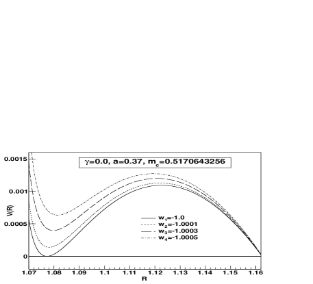
Figure 1: The potential $V(R)$ and the energy conditions EC1$\equiv\rho+p_{r}+2p_{t}$, EC2$\equiv\rho+p_{r}$ and EC3$\equiv\rho+p_{t}$, for $\gamma=0$, $\omega=-1,\;-1.0001,\;-1.0003,\;-1.0005$, $a=0.37$ and $m_{c}=0.5170643256$. Case D: $\omega=-1$

      

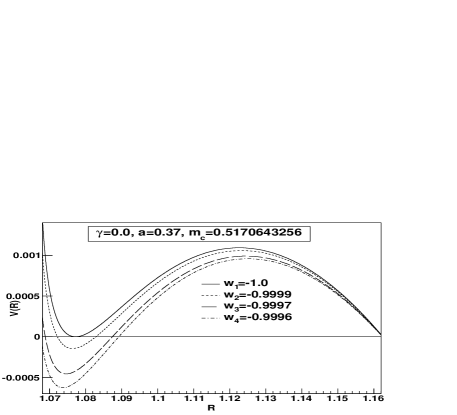
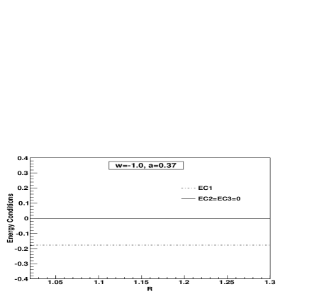
Figure 2: The potential $V(R)$ and the energy conditions EC1$\equiv\rho+p_{r}+2p_{t}$, EC2$\equiv\rho+p_{r}$ and EC3$\equiv\rho+p_{t}$, for $\gamma=0$, $\omega=-1,\;-0.9999,\;-0.9997,\;-0.9996$, $a=0.37$ and $m_{c}=0.5170643256$. Case D: $\omega=-1$

      

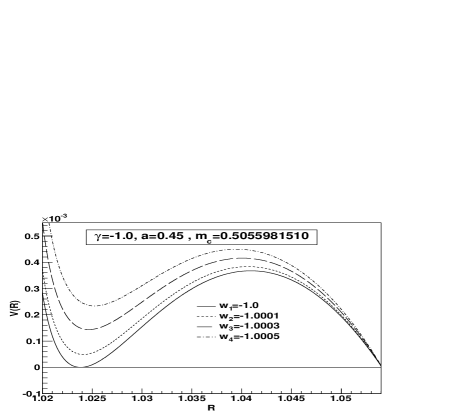
Figure 3: The potential $V(R)$ and the energy conditions EC1$\equiv\rho+p_{r}+2p_{t}$, EC2$\equiv\rho+p_{r}$ and EC3$\equiv\rho+p_{t}$, for $\gamma=0$, $\omega=-1,\;-1.0001,\;-1.0003,\;-1.0005$, $a=0.45$ and $m_{c}=0.5055981510$. Case D: $\omega=-1$

      

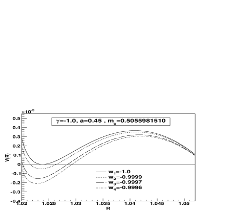
Figure 4: The potential $V(R)$ and the energy conditions EC1$\equiv\rho+p_{r}+2p_{t}$, EC2$\equiv\rho+p_{r}$ and EC3$\equiv\rho+p_{t}$, for $\gamma=-1$, $\omega=-1,\;-0.9999,\;-0.9997,\;-0.9996$, $a=0.45$ and $m_{c}=0.5055981510$. Case D: $\omega=-1$

      

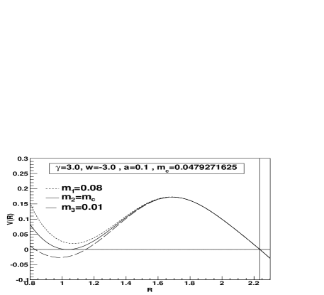
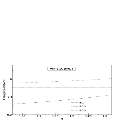
Figure 5: The potential $V(R)$ and the energy conditions EC1$\equiv\rho+p_{r}+2p_{t}$, EC2$\equiv\rho+p_{r}$ and EC3$\equiv\rho+p_{t}$, for $\gamma=3$, $\omega=-3$, $a=0.1$ and $m_{c}=0.0479271625$. The righter vertical straight line denotes the radius of the horizon $R_{h}=1/\sqrt{2a}$. Case I

      

Figure 6: These figures show the dynamical evolution of collapse of a gravastar, forming a ”bounded excursion” gravastar. We have assumed the values $\gamma=3.0$, $\omega=-3.0$, $a=0.1$, $m=0.01$ and initial radius $R_{0}=R(\tau=0)=1.0$.

      

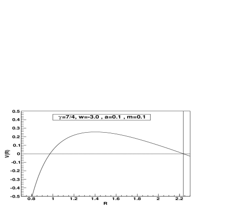
Figure 7: The potential $V(R)$ and the energy conditions EC1$\equiv\rho+p_{r}+2p_{t}$, EC2$\equiv\rho+p_{r}$ and EC3$\equiv\rho+p_{t}$, for $\gamma=7/4$, $\omega=-3$, $a=0.1$ and $m_{c}=0.1$. The righter vertical straight line denotes the radius of the horizon $R_{h}=1/\sqrt{2a}$. Case H

      

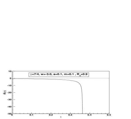
Figure 8: These figures show the dynamical evolution of collapse of a gravastar, forming a black hole. We have assumed the values $\gamma=7/4$, $\omega=-3.0$, $a=0.1$, $m=0.1$ and initial radius $R_{0}=R(\tau=0)=0.9$.

- (1) P.O. Mazur and E. Mottola, ”Gravitational Condensate Stars: An Alternative to Black Holes,” arXiv:gr-qc/0109035; Proc. Nat. Acad. Sci. 101, 9545 (2004) [arXiv:gr-qc/0407075].
- (2) I. Dymnikova and E. Galaktionov, Physics Letters B 645,358 (2007).
- (3) M. Visser and D.L. Wiltshire, Class. Quantum Grav. 21, 1135 (2004)[arXiv:gr-qc/0310107].
- (4) B.M.N. Carter, Class. Quantum Grav. 22, 4551 (2005) [arXiv:gr-qc/0509087].
- (5) A. DeBenedictis, et al, Class. Quantum Grav. 23, 2303 (2006) [arXiv:gr-qc/0511097].
- (6) C.B.M.H. Chirenti and L. Rezzolla, arXiv:0706.1513.
- (7) U. Debnath and S. Chakraborty (2006) [arXiv:gr-qc/0601049].
- (8) P. Rocha, A.Y. Miguelote, R. Chan, M.F.A. da Silva, N.O. Santos,and A. Wang, ”Bounded excursion stable gravastars and black holes,” J. Cosmol. Astropart. Phys. 6, 25 (2008) [arXiv:gr-qc/08034200].
- (9) P. Rocha, R. Chan, M.F.A. da Silva and A. Wang, ”Stable and ”Bounded Excursion” Gravastars, and Black Holes in Einstein’s Theory of Gravity,” J. Cosmol. Astropart. Phys. 11, 10 (2008) [arXiv:gr-qc/08094879].
- (10) R. Chan, M.F.A. da Silva, P. Rocha and A. Wang, ”Stable Gravastars with Anisotropic Dark Energy,” J. Cosmol. Astropart. Phys. 3, 10 (2009) [arXiv:gr-qc/08124924].
- (11) R. Chan, M.F.A. da Silva and P. Rocha, ”How the cosmological constant affects gravastar formation,” J. Cosmol. Astropart. Phys. 12, 17 (2009) [arXiv:gr-qc/09102054].
- (12) R. Chan and M.F.A. da Silva, ”How the charge can affect the formation of gravastars,” J. Cosmol. Astropart. Phys. 7, 29 (2010) [arXiv:gr-qc/10053703].
- (13) R. Chan, M.F.A. da Silva, J.F. Villas da Rocha, Gen. Relat. Grav. 41, 1835 (2009) [arXiv:gr-qc/08033064].
- (14) O. Bertolami and J. Páramos, Phys. Rev. D 72, 123512 (2005) [arXiv:astro-ph/0509547]
- (15) F. Lobo (2007) [arXiv:gr-qc/0611083].
- (16) C. Cattoen, T. Faber and M. Visser, Class. Quantum Grav. 22 4189 (2005).
- (17) V. Dzhunushaliev, V. Folomeev, R. Myrzakulov and D. Singleton, Journal of High Energy Physics 7, 94 (2008), [arXiv:gr-qc/arXiv:0805.3211].
- (18) F. Lobo, Class. Quant. Grav. 23, 1525 (2006).
- (19) K. Lake, Phys. Rev. D 19, 2847 (1979).
- (20) S.W. Hawking and G.F.R. Ellis, The Large Scale Structure of Space-time , Cambridge University Press, Cambridge (1973).
- (21) R. Chan, M.F.A. da Silva and J.F. Villas da Rocha, Mod. Phys. Lett. A, 24, 1137 (2009) [arXiv:gr-qc/0803.2508].
- (22) R.G. Cai and A. Wang (2006) [arXiv:astro-ph/0505136]