We investigate the spontaneous emission spectrum of a qubit in a lossy resonant cavity. We use neither the rotating-wave approximation nor the Markov approximation. The qubit-cavity coupling strength is varied from weak, to strong, even to lower bound of the ultra-strong. For the weak-coupling case, the spontaneous emission spectrum of the qubit is a single peak, with its location depending on the spectral density of the qubit environment. Increasing the qubit-cavity coupling increases the asymmetry (the positions about the qubit energy spacing and heights of the two peaks) of the two spontaneous emission peaks (which are related to the vacuum Rabi splitting) more. Explicitly, for a qubit in a low-frequency intrinsic bath, the height asymmetry of the splitting peaks becomes larger, when the qubit-cavity coupling strength is increased. However, for a qubit in an Ohmic bath, the height asymmetry of the spectral peaks is inverted from the same case of the low-frequency bath, when the qubit is strongly coupled to the cavity. Increasing the qubit-cavity coupling to the lower bound of the ultra-strong regime, the height asymmetry of the left and right peak heights are inverted, which is consistent with the same case of low-frequency bath, only relatively weak. Therefore, our results explicitly show how the height asymmetry in the spontaneous emission spectrum peaks depends not only on the qubit-cavity coupling, but also on the type of intrinsic noise experienced by the qubit.

Keywords: spontaneous emission spectrum, vacuum Rabi splitting, qubit strongly-coupled to a cavity

A qubit strongly-coupled to a resonant cavity: asymmetry of the spontaneous emission spectrum beyond the rotating wave approximation

I Introduction

Strong and ultra-strong qubit-cavity interactions have been achieved in both cavity QED and circuit QED systems (see, e.g., phys-today ; nature-458-178 ; nature-2-81 ; add1 ). This opens up many new possible applications. For example, one could use the cavity as a quantum bus to couple widely-separated qubits in a quantum computer sa ; gr , as a quantum memory to store quantum information, or as a generator and detector of single microwave photons for quantum communications add1 .

As a demonstration of strong interaction in cavity QED and circuit QED systems, the vacuum Rabi splitting has been an exciting subfield of optics and solid-state physics (see, e.g., add2 ; add4 ; pra-69-062320 ; add5 ), after its observation in atomic systems prl-68-1132 . In 2004, two groups nature-432-197 ; nature-432-200  reported the experimental realization of vacuum Rabi splitting  in semiconductor systems: a single quantum dot in a spacer of photonic crystal nanocavity and in semiconductor microcavity, respectively. In the same year, the experiment nature-431-162 showed that the vacuum Rabi splitting can also been obtained in a superconducting two-level system, playing the role of an artificial atom, coupled to an on-chip cavity consisting of a superconducting transmission line resonator. When the qubit was resonantly coupled to the cavity mode, it was observed nature-431-162 that two well-resolved spectral lines were separated by a vacuum Rabi frequency $\nu_{{\mathrm{Rabi}}}\approx 2g.$ Except for the asymmetry in the height of the two split energy-peaks (e.g., Ref. [nature-431-162, ]), the data is in agreement with the transmission spectrum numerically calculated using the rotating wave approximation (RWA). When considering the vacuum Rabi splitting behavior for strong qubit-cavity coupling, the anti-rotating terms should be taken into account, and this might explain the observed asymmetric spontaneous emission (SE) spectrum.

I.1 Antirotating terms are important for strong coupling QED

It is obvious that the anti-rotating terms are not important when the coupling between a qubit and the cavity field is sufficiently weak, and when the energy spacing of the qubit is resonant with the central frequency of the cavity. However, in the ultra-strong coupling regime, the anti-rotating terms of the intrinsic bath of the qubit coupling play an important role prl-98-103602-2007 ; pra-80-033846 ; add8 ; arkiv . As a consequence of the anti-rotating terms in the Hamiltonian of cavity QED and circuit QED, even the ground state of the system contains a finite number of virtual photons. Theoretical research prl-103-147003 ; pra-80-053810 reveal that these virtual photons can be released by a non-adiabatic manipulation, where the Rabi frequency $g(t)$ is modulated in time at frequencies comparable or higher than the qubit transition frequency. This phenomenon, called “emission of the quantum vacuum radiation”, would be completely absent if these anti-rotating terms are neglected. The energy shift of the qubit in its intrinsic bath has been studied in pre-80-021128-2009 using the full description, (i.e., non-Markov and without RWA) and found that the deviations from the previous approximation result already amount to $\sim 5\%$ for $g/\Delta\sim 0.1.$

In doped semiconductor quantum wells embedded in a microcavity (e.g., pra-74-033811 ), considering the anti-rotating coupling of the intracavity photonic mode and the electronic polarization mode, but using RWA in the coupling to their respective environments, it was found pra-74-033811 that for a coherent photonic input, signatures of the ultra-strong coupling have been identified in the asymmetric and peculiar anticrossing of the polaritonic eigenmodes. From the descriptions given above, it can be seen that, as $g/\Delta$ increases to the ultra-strong coupling case, the anti-rotating terms that are otherwise negligible become more relevant and will lead to a profound modification in the nature of the quantum state of the qubit system.

I.2 The asymmetry of the two splitting Rabi peaks can be explained beyond the RWA approximation

In this paper, we study the SE spectrum of a qubit in a cavity. Our calculations include two kinds of anti-rotating terms: one from the intrinsic qubit environment and the other one from the cavity environment. This method is a powerful tool to investigate various kinds of qubit-environment interaction with anti-rotating terms and without using the Markov approximation. Because in this method, the qubit-environment coupling terms higher than the two-order are droped, it constricts that this method is unavailable in the case when the qubit-environment coupling strength is larger than the energy spacing of the qubit add24g ; add25s . Comparing the cases of a qubit in an Ohmic bath with the case of a qubit in a low-frequency bath, we find that for the case of a qubit in a low-frequency bath, as the qubit-cavity coupling strength increases, the height asymmetry of two splitting peaks is enhanced. However, for the case of a qubit in an Ohmic bath, the height asymmetry of the spectral peaks are inverted from the same case of the low-frequency bath, when the qubit is strongly coupled to the cavity. Increasing the qubit-cavity coupling to ultra-strong regime, the height asymmetry of the left and right peaks are inverted, which is consistent with the same case of low-frequency bath, only relatively weak. Since experiments reported that a superconducting qubit intrinsic bath is mainly due to low-frequency noise, our results are consistent with experimental data using a superconducting qubit in Ref. [nature-431-162, ].

We also investigate the dependence of the SE spectrum on the strength of the qubit-cavity coupling and the quality factor $Q$ of the cavity in either an Ohmic or in a low-frequency intrinsic qubit bath. Furthermore, we distinguish the contributions to the asymmetry from each bath: the intrinsic qubit bath and the cavity bath, and clarify the reason for the different kinds of peaks asymmetry. All of these results directly indicate that in the strong coupling regime, the SE spectrum is deeply influenced by the anti-rotating terms and the type of intrinsic noise experienced by the qubit.

II Beyond the Rotating Wave Approximation

By using a cavity to confine the electromagnetic field, the strength of the qubit-cavity interaction can be increased by several orders of magnitude to the regime of strong or even ultra-strong coupling add7 . The strong-coupling regime for cavity quantum electrodynamics has been reached for natural atoms in optical cavities, superconducting qubits in circuit resonators (i.e., on-chip cavities), and quantum dots in photonic-crystal nanocavities. Recently, the ultra-strong coupling regime has be achieved for a superconducting qubit in an on-chip cavity nature-458-178 . Although the coupling of the qubit to the cavity is much stronger than the coupling of the qubit to its intrinsic environment, the parameters in Ref. [nature-431-162, ] show that both the decay rate of the cavity photon ($\kappa/2\pi\approx 0.8$ $\mathrm{MHz}$) and the qubit decoherence rate ($\gamma/2\pi\approx 0.7$ $\mathrm{MHz}$) are comparable. Therefore, we model the environment of the qubit in a cavity using two bosonic baths: one, called the intrinsic bath of the qubit and represented by operators $b_{k}$ and $b_{k}^{\dagger}$, is related to the relaxation of the qubit induced by its intrinsic environment; and the other, denoted as cavity bath of qubit and represented by the operators $a_{k}^{\dagger}$ and $a_{k},$ involves the relaxation of the qubit caused by photons in the cavity. Figure 1 schematically shows the model considered here. For the intrinsic qubit bath, a broad frequency spectrum (e.g., either an Ohmic or a low-frequency spectrum) can be used to characterize it. For the cavity bath, because of the cavity leakage, it can be described by a Lorentzian spectrum with a central frequency, i.e., a single-mode cavity with its frequency broadened by the cavity leakage.

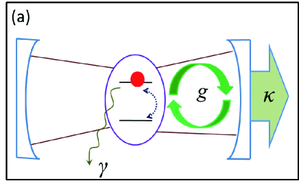
Figure 1: (Color online) Schematic diagram of a two-level system or qubit with dissipation rate $\gamma,$ which is coupled to a cavity with loss rate $\kappa$ by the qubit-cavity coupling strength $g.$

The Hamiltonian can be written (throughout this paper, we choose $\hbar=1$) pra-74-033811 as

$$H = \frac{1}{2}\Delta\sigma_{z}+\sum_{k}\omega_{k,1}a_{k}^{\dagger}a_{k}+\sum_{k}g_{k,1}(a_{k}^{\dagger}+a_{k})\sigma_{x}$$

$$+\sum_{k}\omega_{k,2}b_{k}^{\dagger}b_{k}+\sum_{k}g_{k,2}(b_{k}^{\dagger}+b_{k})\sigma_{x},$$

where $\sigma_{x}=\sigma_{+}+\sigma_{-}$ and $i=1,2$, denote the intrinsic and cavity baths of the qubit, respectively.

The baths experienced by the qubit can be characterized by a spectral density $J_{i}(\omega)=\sum_{k}g_{k,i}^{2}\delta(\omega-\omega_{k,i}).$ To deal with the anti-rotating terms in Eq. (II), we will perform a unitary transformation on the Hamiltonian. This unitary transformation is applied to the Hamiltonian $H$ as follows:

$$H^{\prime}=\exp(S)H\exp(-S),$$ (2)

with $S=S_{1}+S_{2},$ where $S_{i}$ ($i=1,2$) is given by

$$S_{1} = \sum_{k}\frac{g_{k,1}}{\omega_{k,1}}\;\xi_{k,1}\left(a_{k}^{\dagger}-a_{k}\right)\sigma_{x},$$ (3)

$$S_{2} = \sum_{k}\frac{g_{k,2}}{\omega_{k,2}}\;\xi_{k,2}\left(b_{k}^{\dagger}-b_{k}\right)\sigma_{x}.$$ (4)

In Eq. (3, 4), the parameter $\xi_{k,j}=\omega_{k,j}/(\omega_{k,j}+\eta_{j}\,\Delta)$ is a $k$-dependent variable. Up to order $g_{k,i}$, the transformed Hamiltonian $H^{(1)}$ can be written as

$$H^{\prime} \approx \frac{1}{2}\eta\,\Delta\sigma_{z}+\sum_{k}\omega_{k,1}a_{k}^{\dagger}a_{k}+\sum_{k}\omega_{k,2}b_{k}^{\dagger}b_{k}$$ (5)

$$+\sum_{k}\tilde{g}_{k,1}\left(a_{k}^{\dagger}\sigma_{-}+a_{k}\sigma_{+}\right)$$

$$+\sum_{k}\tilde{g}_{k,2}\left(b_{k}^{\dagger}\sigma_{-}+b_{k}\sigma_{+}\right),$$

where

$$\tilde{g}_{k,i}=\left(\frac{2\eta_{i}\,\Delta}{\omega_{k,i}+\eta_{i}\,\Delta}\right)g_{k,i},$$ (6)

$$\eta=\eta_{1}\,\eta_{2},$$ (7)

$$\eta_{i}=\exp\left(-\sum_{k}\frac{2g_{k,i}^{2}{}}{\omega_{k,i}^{2}}\;\xi_{k,i}^{2}{}\right),$$ (8)

and $\eta=\eta_{1}\eta_{2}.$ Now the transformed Hamiltonian (5) has the same form as the Hamiltonian under the RWA, but its parameters have been renormalized to include the effects of the anti-rotating terms related with the intrinsic and cavity baths of the qubit. From the transformed Hamiltonian $H^{\prime},$ one can see that, based on energy conservation, the ground state of the transformed Hamiltonian $H^{\prime}$ is

$$\left|g^{\prime}\right\rangle=\left|\downarrow\right\rangle\otimes\prod\limits_{k}\left|0_{k,1},0_{k,2}\right\rangle,$$ (9)

(using $\sigma_{z}\left|\downarrow\right\rangle=-\left|\downarrow\right\rangle$) and the corresponding ground-state energy is $-\eta\;\Delta/2$. Therefore, the ground state of the original Hamiltonian $H$ is given by

$$\left|g\right\rangle=\exp\left(-S\right)\left|g^{\prime}\right\rangle,$$ (10)

which is the dressed state of the qubit and the environment due to the anti-rotating terms prl-103-147003 ; pra-80-053810 .

A qubit can experience different types of intrinsic baths. The most commonly-used bath is the photon or phonon bath, which can be described by an Ohmic spectrum. However, for many solid-state qubits (e.g., superconducting qubits), the dominant dissipation can be due to two-level fluctuators, which behave like a low-frequency bath addie . Here we consider either an Ohmic or a low-frequency intrinsic bath. The Ohmic bath with Drude cutoff is given by

$$J_{1}^{\mathrm{Ohm}}(\omega)=\frac{2\alpha_{\mathrm{Ohm}}\omega}{1+\left(\omega/\omega_{\mathrm{Ohm}}\right)^{2}},$$ (11)

where $\omega_{\mathrm{Ohm}}$ is the high-frequency cutoff and $\alpha_{\mathrm{Ohm}}$ a dimensionless parameter characterizing the coupling strength between the qubit and its intrinsic bath. Here the low-frequency bath is written as

$$J_{1}^{\mathrm{low}}(\omega)=\frac{2\alpha_{\mathrm{low}}\omega}{\left(\omega/\Delta\right)^{2}+\left(\omega_{\mathrm{low}}/\Delta\right)^{2}},$$ (12)

where $\omega_{\mathrm{low}}$ is a characteristic frequency lower than the qubit energy spacing $\Delta$ of the qubit, and $\alpha_{\mathrm{low}}$ is a dimensionless coupling strength between the qubit and its intrinsic bath. If $\omega\geq\omega_{\mathrm{low}}$, $J_{1}^{\mathrm{low}}(\omega)\sim 1/\omega$, corresponding to $1/f$ noise.

For a lossy cavity, the bath can be described by a Lorentzian spectral density with a central frequency pra-79-042302 :

$$J_{2}(\omega)=\frac{g^{2}\lambda}{\pi[(\omega-\omega_{\mathrm{cav}})^{2}+\lambda^{2}]},$$ (13)

which corresponds to a single-mode cavity, with its frequency broadened by the cavity loss. In Eq. (13), $\lambda$ is the frequency width of the cavity bath density spectrum, $\omega_{\mathrm{cav}}$ is the central frequency of the cavity mode, and $g$ denotes the coupling strength between the qubit and the cavity. Also, the parameter $\lambda$ is related to the cavity bath correlation time and $\omega_{\mathrm{cav}}/\lambda$ is the quality factor $Q$ of the cavity.

Using $J_{i}(\omega)=\sum g_{k,i}^{2}\delta(\omega-\omega_{k,i}),$ one can derive from Eq. (8) that $\eta_{i}$ is determined self-consistently by the equation

$$\log\eta_{i}+\int\limits_{0}^{\infty}\ \frac{2J_{i}(\omega)d\omega}{(\omega+\eta_{i}\,\Delta)^{2}}=0.$$ (14)

Below we will solve the equation of motion for the density matrix in Hamiltonian (II) and obtain the qubit SE spectrum.

II.1 Equation of Motion for the Density Matrix

The equation of motion of the density matrix $\rho_{SB}$ for the whole system, i.e., qubit system ($S$) and bath ($B$) is given by

$$\frac{d}{dt}\rho_{SB}(t)=-i[H,\rho_{SB}(t)].$$ (15)

After the unitary transformation (2), we have

$$\frac{d}{dt}\rho_{SB}^{\prime}(t)=-i[H^{\prime},\rho_{SB}^{\prime}(t)],$$ (16)

where $\rho_{SB}^{\prime}=\exp(S)\rho_{SB}\exp(-S)$ is the density matrix of the whole system in the Schrödinger picture with the transformed Hamiltonian $H^{\prime}$ [i.e., Eq. (5)]. Below we solve the transformed equation of motion, Eq. (16), in the interaction picture with $H_{0}=\eta\,\Delta\sigma_{z}/2+\sum_{k,i}\omega_{k,i}a_{k,i}^{\dagger}a_{k,i}$. In this interaction picture, the transformed Hamiltonian $H^{\prime}$ can be written as

$$V_{I}^{\prime}(t)=\sum_{k,i}\tilde{g}_{k,i}a_{k,i}^{\dagger}\sigma_{-}\exp\left[i(\omega_{k,i}-\eta\,\Delta)t\right]+\mathrm{H.c}.$$ (17)

The equation of motion for the density matrix $\rho_{SB}^{\prime I}(t)$ of the whole system ($S$+$B$) can be written as

$$\frac{d}{dt}\rho_{SB}^{\prime I}(t)=-i[V_{I}^{\prime}(t),\rho_{SB}^{\prime I}(t)].$$ (18)

with $\rho_{SB}^{\prime I}(t)=\exp\left(iH_{0}t\right)\rho_{SB}^{\prime}(t)\exp\left(-iH_{0}t\right).$

Integrating Eq. (18), we have

$$\rho_{SB}^{\prime I}(t)=\rho_{SB}^{\prime I}(t_{i})-i\int\limits_{t_{0}}^{t}[V_{I}^{\prime}(t^{\prime}),\rho_{SB}^{\prime I}(t^{\prime})]dt^{\prime},$$ (19)

where $t_{0}$ is the initial time for the qubit-environment interaction to turn on. Here we choose $t_{0}=0.$ Substituting $\rho_{SB}^{\prime I}(t)$ into Eq. (18), we obtain the equation of motion as

$$\frac{d}{dt}\rho_{SB}^{\prime I}(t) = -i[V_{I}^{\prime}(t),\rho_{SB}^{\prime}(0)]$$

$$-\int\limits_{0}^{t}[V_{I}^{\prime}(t),[V_{I}^{\prime}(t^{\prime}),\rho_{SB}^{\prime I}(t^{\prime})]]dt^{\prime}.$$

Using the Born approximation F1 , the density matrix $\rho_{SB}^{\prime I}(t)$ in Eq. (II.1) can be approximated by $\rho_{SB}^{\prime I}(t)=\rho_{S}^{\prime I}(t)\rho_{B}(0).$ Tracing over the degrees of freedom of the two baths, one obtain

$$\frac{d}{dt}\rho_{S}^{\prime I}(t) = -i\mathrm{Tr}_{R}[V_{I}^{\prime}(t),\rho_{S}^{\prime}(0)\otimes\rho_{B}^{\prime}(0)]$$

$$-\mathrm{Tr}_{R}\int\limits_{0}^{t}[V_{I}^{\prime}(t),[V_{I}^{\prime}(t^{\prime}),\rho_{S}^{\prime I}(t^{\prime})\otimes\rho_{B}(0)]]dt^{\prime},$$

where $\rho_{S}^{\prime I}(t)=\mathrm{Tr}_{R}\left[\rho_{SB}^{\prime I}(t)\right].$ Because the two bosonic baths are assumed to be in thermal equilibrium, it follows from the Bose-Einstein distribution that

$$\mathrm{Tr}_{R}\left(a_{k,i}^{\dagger}a_{k,i}\rho_{B}\right) = n_{k,i},$$ (22)

$$\mathrm{Tr}_{B}\left(a_{k,i}a_{k,i}^{\dagger}\rho_{B}\right) = n_{k,i}+1,$$ (23)

where $n_{k,i}$ is the thermal average boson number at mode $k$. Then, substituting $V_{I}^{\prime}(t)$ into Eq. (II.1), we have

$$\frac{d}{dt}\rho_{S}^{\prime I}(t)$$

$$= -\sum_{k,i}\tilde{g}_{k,i}^{2}\int\limits_{0}^{t}f\!\left(t^{\prime}\right)\exp\left[i(\omega_{k,i}-\eta\,\Delta)(t-t^{\prime})\right]dt^{\prime}-\mathrm{H.c.}$$

where

$$f\left(t^{\prime}\right)\! \!=\! \!n_{k,i}\left[\sigma_{-}\sigma_{+}\rho_{S}^{\prime I}\left(t^{\prime}\right)-\sigma_{+}\rho_{S}^{\prime I}(t^{\prime})\sigma_{-}\right]$$

$$\!+\left(n_{k,i}+1\right)\left[\rho_{S}^{\prime I}(t^{\prime})\sigma_{+}\sigma_{-}-\sigma_{-}\rho_{S}^{\prime I}(t^{\prime})\sigma_{+}\right].$$

On the right-hand side of Eq. (II.1), the terms related with $n_{k,i}$ and $n_{k,i}+1$ describe, respectively, the decay and excitation processes, with the rates depending on the temperature. Here, for simplicity, we study the zero-temperature case with $n_{k,i}=0,$ i.e., only the spontaneous decay occurs, which corresponds to a purely dissipative process. The appendix gives the solution of Eq. (II.1) for the reduced density matrix $\rho_{S}^{\prime I}(t)$ of the qubit in the interaction picture. With the solution for $\rho_{S}^{\prime I}(t),$ one can derive the reduced density matrix $\rho_{S}^{\prime}(t)$ of the qubit in the Schrödinger picture:

$$\rho_{S}^{\prime}(t) = \exp\left(i\eta\,\Delta\sigma_{z}t/2\right)\rho_{S}^{\prime I}(t)\exp\left(i\eta\,\Delta\sigma_{z}t/2\right)$$ (26)

$$= \left(\begin{array}[]{cc}\mathcal{L}^{-1}\left[\frac{\rho_{22}^{\prime}(0)}{p+A_{+}+A_{-}}\right]&\mathcal{L}^{-1}\left[\frac{\rho_{21}^{\prime}(0)}{p+A_{+}}\right]\mathrm{e}^{-it\text{$\Delta$}\text{$\eta$}}\\ \mathcal{L}^{-1}\left[\frac{\rho_{12}^{\prime}(0)}{p+A_{-}}\right]\mathrm{e}^{it\text{$\Delta$}\text{$\eta$}}&\mathcal{L}^{-1}\left[\frac{\rho_{{}_{22}}^{\prime}(0)}{p}-\frac{\rho_{{}_{22}}^{\prime}(0)}{p+A_{+}+A_{-}}+\frac{\rho_{{}_{11}}^{\prime}(0)}{p}\right]\end{array}\right).$$ (29)

Because the reduced density matrix $\rho_{S}(t)$ in the Schrödinger picture with the original Hamiltonian $H$ [i.e. Eq. (II)] is related to $\rho_{S}^{{}^{\prime}}(t)$ by the relation

$$\rho_{S}(t)=\mathrm{Tr}_{B}\left[\exp\left(-S\right)\rho_{S}^{\prime}(t)\rho_{B}\exp\left(S\right)\right].$$ (30)

Then, using $\exp\left(S\right)=\cosh Y+\sigma_{x}\sinh Y$, with $Y=\sum_{k,i}g_{k,i}\xi_{k,i}(a_{k,i}^{\dagger}-a_{k,i})/\omega_{k,i}$, and tracing over the degrees of freedom of the two baths, we obtain

$$\rho_{S}(t)=\frac{1+\eta}{2}\rho_{S}^{\prime}(t)+\frac{1-\eta}{2}\sigma_{x}\,\rho_{S}^{\prime}(t)\,\sigma_{x}.$$ (31)

II.2 Derivation of the spontaneous Emission Spectrum

When measured by an ideal system with negligible bandwidth, the spontaneous emission spectrum can be given by hjc

$$P(\omega)\propto\int\limits_{0}^{\infty}\!\!dt\int\limits_{0}^{\infty}\!\!dt^{\prime}\exp\left[-i\omega(t-t^{\prime})\right]C(t,t^{\prime}),$$ (32)

with the two-time correlation function

$$C(t,t^{\prime}) = \left\langle\sigma_{+}(t)\sigma_{-}(t^{\prime})\right\rangle$$

$$= \left\langle\psi(0)\right|\sigma_{+}(t)\sigma_{-}(t^{\prime})\left|\psi(0)\right\rangle,$$

where the $\sigma_{\pm}(t)=\exp\left(iHt\right)\sigma_{\pm}\exp\left(-iHt\right)$ are the raising ($+$) and lowering ($-$) Pauli matrices in the Heisenberg picture and $\left|\psi(0)\right\rangle$ is the initial state of the whole system, which remains unchanged in the Heisenberg picture. Using $\left|\psi^{\prime}(0)\right\rangle=\exp\left(S\right)\left|\psi(0)\right\rangle,$ the two-time correlation function can be written as

$$C(t,t^{\prime})=\left\langle\psi^{\prime}(0)\right|\mathrm{e}^{iH^{\prime}t}\sigma_{+}^{\prime}\mathrm{e}^{-iH^{\prime}t}\mathrm{e}^{iH^{\prime}t^{\prime}}\sigma_{-}^{\prime}\mathrm{e}^{-iH^{\prime}t^{\prime}}\left|\psi^{\prime}(0)\right\rangle,$$ (34)

where $\sigma_{\pm}^{\prime}=\exp\left(S\right)\sigma_{\pm}\exp\left(-S\right)$. Because the zero-temperature case is considered here, this two-time correlation function can be approximated as

$$C(t,t^{\prime})\approx\left\langle\psi^{\prime}(0)\right|\mathrm{e}^{iH^{\prime}t}\tilde{\sigma}_{+}^{\prime}\mathrm{e}^{-iH^{\prime}t}\mathrm{e}^{iH^{\prime}t^{\prime}}\tilde{\sigma}_{-}^{\prime}\mathrm{e}^{-iH^{\prime}t^{\prime}}\left|\psi^{\prime}(0)\right\rangle,$$ (35)

with

$$\tilde{\sigma}_{\pm}^{\prime} = \prod\limits_{k}\left\langle 0_{k^{\prime},1},0_{k^{\prime},2}\right|\sigma_{\pm}^{\prime}\left|0_{k,1},0_{k,2}\right\rangle$$ (36)

$$= \frac{1+\eta}{2}\;\sigma_{\pm}+\frac{1-\eta}{2}\;\sigma_{\mp}.$$

In deriving Eq. (36), the two baths are assumed in the ground state for the zero-temperature case. Therefore, from Eq. (36), we have

$$C(t,t^{\prime})\approx\left(\frac{1+\eta}{2}\right)^{2}\left\langle\sigma_{+}\left(t\right)\sigma_{-}\left(t^{\prime}\right)\right\rangle_{H^{\prime}}$$

$$+\frac{1-\eta^{2}}{4}\left(\left\langle\sigma_{+}\left(t\right)\sigma_{+}\left(t^{\prime}\right)\right\rangle_{H^{\prime}}+\left\langle\sigma_{-}\left(t\right)\sigma_{-}\left(t^{\prime}\right)\right\rangle_{H^{\prime}}\right)$$

$$+\left(\frac{1-\eta}{2}\right)^{2}\left\langle\sigma_{-}\left(t\right)\sigma_{+}\left(t^{\prime}\right)\right\rangle_{H^{\prime}},$$ (37)

where the expectation value of the operator in the transformed Hamiltonian $H^{\prime}$ is

$$\left\langle\sigma_{\alpha}\left(t\right)\sigma_{\beta}\left(t^{\prime}\right)\right\rangle_{H^{\prime}}$$

$$= \left\langle\psi^{\prime}(0)\right|\mathrm{e}^{iH^{\prime}t}\sigma_{\alpha}^{\prime}\mathrm{e}^{-iH^{\prime}t}\mathrm{e}^{iH^{\prime}t^{\prime}}\sigma_{\beta}^{\prime}\mathrm{e}^{-iH^{\prime}t^{\prime}}\left|\psi^{\prime}(0)\right\rangle,$$

with $\alpha,\beta=\pm.$

In our case, $\eta$ is very close to $1$. Therefore, Eq. (37) can be further approximated as

$$C(t,t^{\prime})\approx C(t,t^{\prime})_{H^{\prime}},$$ (39)

with $C(t,t^{\prime})_{H^{\prime}}=$ $\left\langle\sigma_{+}\left(t\right)\sigma_{-}\left(t^{\prime}\right)\right\rangle_{H^{\prime}}.$ For a qubit state specified by a density matrix $\rho(t),$ we can formulate the expectation values of $\sigma_{+}(t),$ $\sigma_{-}(t)$ and $\sigma_{+}(t)\sigma_{-}(t)$ by the matrix elements, $\left\langle\sigma_{+}(t)\right\rangle=\left\langle\sigma_{-}(t)\right\rangle^{\ast}=\rho_{21}(t)$ and $C(t,t)=\rho_{11}(t).$ According to the quantum regression theorem hjc , the correlation function becomes

$$C(t,t+\tau)_{H^{\prime}}$$

$$= \mathcal{L}^{-1}\left(\frac{1}{p+A_{+}}\right)_{\!\tau}\mathrm{e}^{-i\Delta\eta\text{$\tau$}}\rho_{11}^{\prime}(t).$$

In a spontaneous emission process, the initial state is an excited state $\left|\psi(0)\right\rangle=\exp\left(-S\right)\left|\uparrow\right\rangle\otimes\prod\limits_{k}\left|0_{k,1},0_{k,2}\right\rangle$, which can be achieved by $\sigma_{x}\left|g\right\rangle.$ Then, the initial state in the transformed Hamiltonian (5) is $\left|\psi^{\prime}(0)\right\rangle=\left|\uparrow\right\rangle\otimes\prod\limits_{k}\left|0_{k,1},0_{k,2}\right\rangle,$ i.e. $\rho_{11}^{\prime}=1.$ Therefore, from Eq. (A.12) in the Appendix A, the dynamics evolution of $\rho_{11}^{\prime}$ can be expressed as

$$\rho_{11}^{\prime}(t)=\mathcal{L}^{-1}\left(\frac{1}{p+A_{+}+A_{-}}\right)_{\!t}.$$ (41)

Using the Schrödinger equation (see Appendix B) pra77 , we have

$$\mathcal{L}^{-1}\left(\frac{1}{p+A_{+}+A_{-}}\right)_{\!t}$$

$$= \mathcal{L}^{-1}\left(\frac{1}{p+A_{+}}\right)_{\!t}\times\mathcal{L}^{-1}\left(\frac{1}{p+A_{-}}\right)_{\!t},$$

where $\mathcal{L}^{-1}\left(\frac{1}{p+A_{+}}\right)$ and $\mathcal{L}^{-1}\left(\frac{1}{p+A_{-}}\right)$ are conjugate quantities (see Appendix A). From

$$C(t,t+\tau)_{H^{\prime}}$$

$$= \mathrm{e}^{-i\text{$\Delta$}\text{$\eta$}\left(\text{$\tau+t$}\right)}\mathcal{L}^{-1}\left(\frac{1}{p+A_{+}}\right)_{\!\left(\tau+t\right)}\!\times\mathcal{L}^{-1}\left(\frac{1}{p+A_{-}}\right)_{\!t}e^{i\text{$\Delta$}\text{$\eta$}t},$$

we obtain the two-time correlation function for any $t$ and $t^{\prime}$,

$$C(t,t^{\prime})_{H^{\prime}} = \mathcal{L}^{-1}\left(\frac{1}{p+A_{+}}\right)_{\!t}\mathrm{e}^{-i\text{$\Delta$}\text{$\eta$}t}$$

$$\times\mathcal{L}^{-1}\left(\frac{1}{p+A_{-}}\right)_{\!t^{\prime}}\mathrm{e}^{-i\text{$\Delta$}\text{$\eta$}t^{\prime}}.$$

Finally, using the Wiener-Khinchin theorem, the SE spectrum is given by

$$P(\omega) \propto \int\limits_{0}^{\infty}\!\!dt\int\limits_{0}^{\infty}\!\!dt^{{}^{\prime}}\exp\left[-i\omega(t-t^{{}^{\prime}})\right]C(t,t^{{}^{\prime}})$$

$$= \left|\mathcal{F}\left[\mathcal{L}^{-1}\left(\frac{1}{p+A_{+}}\right)\mathrm{e}^{-i\text{$\Delta$}\text{$\eta\tau$}}\right]\right|^{2}$$

$$= \frac{1}{\left[\omega-\Delta\eta-R\left(\omega\right)\right]^{2}+\Gamma\left(\omega\right)^{2}}.$$

III Dependence of the spontaneous emission spectrum on the baths

We will show the SE spectrum of the qubit in resonance with the cavity central frequency ($\Delta=\omega_{\mathrm{cav}}$) as a function of the microwave probe frequency for three cases: weak, strong and ultra-strong qubit-cavity couplings.

Weak coupling means the qubit-cavity coupling strength $g$ is less than the sum of the dissipation rate of the qubit and the cavity. The dissipation rates of the qubit due to its intrinsic bath is approximately denoted as $\Gamma_{\mathrm{qb}},$ which can be $\Delta\>\alpha_{\mathrm{Ohm}}$ or $\Delta\>\alpha_{\mathrm{low}}.$ And the dissipation rate due to the cavity bath can be approximately as the spectrum width of the cavity spectral density $\lambda.$ So  weak coupling is express as $g<\left(\Gamma_{\mathrm{qb}}+\lambda\right).$

Strong coupling means that the qubit-cavity coupling strength $g$ is larger than the sum of the dissipation rate of the qubit and the cavity: $g>\left(\Gamma_{\mathrm{qb}}+\lambda\right)$, but it is typically two orders of magnitude smaller than the qubit energy spacing $\Delta$ and the cavity frequency $\omega_{\mathrm{cav}}$, i.e., $g\sim 10^{-2}\Delta,$ such as the case in Ref. [nature-431-162, ].

Ultra-strong coupling means that the qubit-cavity coupling $g$ is to a significant fraction of the transition frequency $\Delta$ (e.g., $g\gtrsim 0.1\Delta$). This case extends to the fine-structure limit for the maximal value of an electric-dipole coupling.

The energy spectral density of a bath plays an important role in determining the energy-shift direction and the asymmetry of the SE spectrum. In Fig. 2, we show the spectral densities for both intrinsic and cavity baths of the qubit. For the intrinsic bath of the qubit, both a low-frequency bath and an Ohmic bath are considered. The spectral density of the cavity bath is symmetric about the central frequency $\omega_{{}_{\mathrm{cav}}}$ of the cavity.

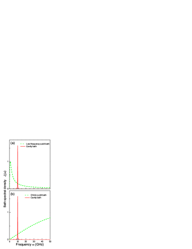
Figure 2: (Color online) The spectrum density of the qubit environment. (a) Lorentzian cavity bath and low-frequency intrinsic bath of the qubit. (b) Lorentzian cavity bath and Ohmic intrinsic bath of the qubit. From Fig. (a) and (b), we see that the dominant regimes of the low-frequency and Ohmic qubit bath spectral density are different.

Considering the experimental parameters nature-431-162 ; add9 , we assume the qubit energy spacing to be$\ \Delta=10$ $\mathrm{GHz}$. The dimensionless coupling strength $\alpha$ between the qubit and its intrinsic bath (either Ohmic- or low-frequency bath) is fixed at $\alpha=10^{-4},$ which implies that the decay rate of the intrinsic bath is $\Gamma_{\mathrm{qb}}\sim 1$ $\mathrm{MHz}.$

III.1 Effect of the cavity bath on the spontaneous emission spectrum

To illustrate the effect of the cavity bath with a symmetric spectral density, in Fig. 3 we show the qubit SE spectrum when only the cavity bath is present. To enhance these features further, we choose a low quality factor $Q=10^{2}$, and plot the SE spectra in Fig. 3(a) for strong ($g=10^{2}$ $\mathrm{MHz}$) and ultrastrong ($g=$ $10^{3},$ $2\times 10^{3}$ $\mathrm{MHz}$) qubit-cavity coupling. Due to the scope of application of this method, only the lower bound of the ultra-strong coupling $g=$ $0.1\Delta$ and $g=0.2\Delta$ are considered. As a comparison, the results under the RWA are given in Fig. 3(b). Also, the SE spectra without and with RWA for $Q=10^{3}$ are plotted in Fig. 3(c,d). In the case of strong qubit-cavity coupling, the two peaks of the vacuum Rabi splitting are nearly symmetric about $\omega=\Delta$, almost coinciding with the results under the RWA. When the qubit-cavity coupling increases, the height and the position asymmetry (about qubit energy spacing $\Delta$) of the two peaks  becomes more apparent, in sharp contrast to the symmetric SE peaks obtained under RWA [see Fig. 3(a,b) and (c,d)]. As we know, if the RWA is used, the qubit-cavity coupling term $\sum\limits_{k}g_{k,2}(a_{k,2}^{\dagger}+a_{k,2})(\sigma_{+}+\sigma_{-})$ in the Hamiltonian $H$ becomes $\sum\limits_{k}g_{k,2}(a_{k,2}^{\dagger}\sigma_{-}+a_{k,2}\sigma_{+})$. The energy spectral density in the regions lower and higher than the central frequency of the cavity (related to absorbing and emitting a single photon in the cavity) are identical. Therefore, when the qubit energy spacing is in resonance with the cavity central frequency, the coupling strength is symmetric about the qubit energy spacing for the absorption and emission processes.

While taking into account the anti-rotating terms, the coupling term becomes $\sum\limits_{k}\tilde{g}_{k,2}(a_{k,2}^{\dagger}\sigma_{-}+a_{k,2}\sigma_{+})$ in the transformed Hamiltonian $H^{\prime}$, with a renormalized coupling strength $\tilde{g}_{k,2}=2\eta_{2}\,\Delta g_{k,2}/\left(\omega_{k,2}+\eta_{2}\,\Delta\right)$ . Obviously, the renormalized coupling strength $\tilde{g}_{k,2}$ induces the spectral asymmetry: for a symmetric spectral density of the cavity bath , in the region $\omega_{k,2}<\Delta$, due to $2\eta_{2}\,\Delta/\left(\omega_{k,2}+\eta_{2}\,\Delta\right)>1,$ the renormalized interaction $\tilde{g}_{k,2}$ is larger than $g_{k,2}$. However, in the region $\omega_{k,2}>\Delta,$ owing to $2\eta_{2}\,\Delta/\left(\omega_{k,2}+\eta_{2}\,\Delta\right)<1,$ the effective coupling strength $\tilde{g}_{k,2}$ is smaller than $g_{k,2}$.

These results (with and without the RWA) indicate that the RWA cannot be used in the range of ultrastrong qubit-cavity coupling. The general tendency observed here is that the RWA overestimates the frequency shift in the low-energy regime $\omega\sim-g$, while it under-estimates the frequency shift in the high-energy regime $\omega\sim g.$ Our results are consistent with the results in Ref. [pra-80-033846, ].

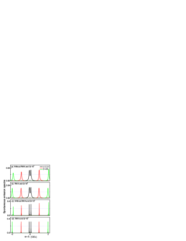
Figure 3: (Color online) Spontaneous emission spectra of the qubit only in the cavity bath (symmetric spectral density). Figure (a) and (c) are the results without RWA with $Q=10^{2}$ and $Q=10^{3}$. Figures (b) and (d) are the results of the RWA with $Q=10^{2}$ and $Q=10^{3}$. To see the height asymmetry of two peaks clearly, the horizontal grid lines are plotted as reference. Note that in (a) and (c), the two peaks of spontaneous emission spectrum present obvious height and position asymmetry (about $\omega=\Delta$) in ultra-strong qubit-cavity coupling.

III.2 Combined effect of both intrinsic and cavity baths on the spontaneous emission spectrum

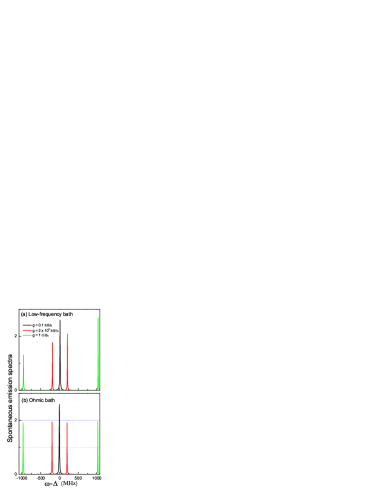
Figure 4: (Color online) Spontaneous emission spectra of the qubit in resonance with the central frequency $\omega_{{}_{\mathrm{cav}}}$ of the cavity for weak, strong and the lower bound of the ultra-strong qubit-cavity interactions. The cavity quality factor is $Q=10^{4}$. (a) coupling strength to the low-frequency intrinsic bath of the qubit $\alpha_{\mathrm{low}}=10^{-4}$, (b) coupling strength to the Ohmic intrinsic bath of the qubit $\alpha_{\mathrm{Ohm}}=10^{-4}$. To see the height asymmetry of the peaks clearly, the horizontal grid lines are plotted as reference. Note that (a) demonstrates the obvious height asymmetry in the case of strong and ultra-strong qubit-cavity coupling and the asymmetry increases as the qubit-cavity coupling grows. Figure (b) shows inverted height asymmetry of two peaks from (a) in the strong qubit-cavity coupling case, but as the qubit-cavity coupling increases to the ultra-strong regime, the height asymmetry of the right and left spectral peaks are inverted.

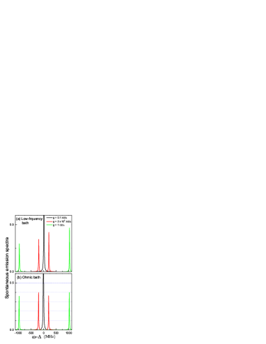
Figure 5: (Color online) Spontaneous emission spectra of the qubit in resonance with the central frequency $\omega_{{}_{\mathrm{cav}}}$ of cavity for weak, strong and the lower bound of the ultra-strong qubit-cavity interactions. The cavity quality factor is $Q=10^{3}$. (a) coupling strength to the low-frequency intrinsic bath of the qubit $\alpha_{\mathrm{low}}=10^{-4}$, (b) coupling strength to the Ohmic intrinsic bath of the qubit $\alpha_{\mathrm{Ohm}}=10^{-4}$. To see clearly the height asymmetry of the peaks, horizontal grid lines are plotted as reference. Note that (a) demonstrates an obvious height asymmetry in the case of strong and ultra-strong qubit-cavity coupling and the asymmetry increases as the qubit-cavity coupling grows. Figure (b) shows the inverted height asymmetry of two peaks from (a) in the strong qubit-cavity coupling case, but as the qubit-cavity coupling increases to the ultra-strong regime, the height asymmetry of the right and left spectral peaks are inverted.

Although a high-$Q$ seems plausible for minimizing the loss of the cavity, it limits the measurement speed. Here, we consider a cavity with the quality factor pra-69-062320 ; nature-431-162 $Q=10^{4}$ in the presence of a qubit (see Fig. 4). We also plot the SE spectrum for $Q=$ $10^{3}$ in Fig. 5, and see how the quality factor affects the results. The dissipation rate of the cavity is approximately to the spectral width $\lambda$ of the cavity bath. If $Q=10^{4},$ the dissipation rate of the cavity bath is about $1$ $\mathrm{MHz}$ (the same order of magnitude of the bath dissipation rate). Figures 4(a) and 4(b) show the spectra of the qubit coupled with a low-frequency and an Ohmic intrinsic baths, respectively. From Fig. 4(a), we see that in the case of weak qubit-cavity coupling $g=10^{-5}\Delta=0.1$ $\mathrm{MHz}$, the SE spectrum is a single peak with the central frequency larger than the energy spacing $\Delta$ of the bare qubit, which corresponds to a blue-shift. In the case of strong qubit-cavity coupling, $g=2\times 10^{-2}\Delta=2\times 10^{2}$ $\mathrm{MHz}$, the SE spectrum shows the vacuum Rabi splitting, with the two height asymmetric peaks, just as shown in Ref. [nature-431-162, ]. By further increasing the qubit-cavity coupling $g=10^{-1}\Delta=1$ $\mathrm{GHz},$ not only the height of the SE peaks but also their positions demonstrate a strong asymmetry about $\omega=\Delta$. The qubit-cavity coupling strength $g=10^{-1}\Delta$ is the lower bound of the ultra-strong coupling regime.

Figure 4(b) shows the SE spectrum of a qubit in the Ohmic intrinsic bath. For a weak qubit-cavity coupling, the central frequency of the SE spectrum shifts to an energy slightly lower than the energy spacing $\Delta$ of the bare qubit, which corresponds to a red-shift. This energy-shift direction is opposite to the case when the qubit is in a low-frequency intrinsic bath [see Fig. 4(a)], and the energy shift is smaller. For a strong qubit-cavity coupling, the two SE peaks also show a weak asymmetry , with the left peak higher than the right peak. This peak asymmetry is inverted from the same case in Fig. 4(a). As the qubit-cavity coupling increases to the ultra-strong regime, the height asymmetry of the left and right SE spectrum are inverted [see Fig. 4(b)]. The SE spectra of the qubit in a cavity with quality factor $Q=10^{3}$ are shown in Fig. 5, which present nearly the same features as in Fig. 4, in addition to the broader SE peaks in Fig. 5. This is because of an increased dissipation rate of the qubit induced by a larger cavity dissipation rate. These results are briefly summarized in table I.

Table 1: Summary of our main results for the spontaneous emission spectra in the case of weak, strong and ultra-strong qubit-cavity coupling. The spectra with symmetric peaks (S), height asymmetric peaks (AS) and very asymmetric peaks (VAS) are abbreviated as S, AS and VAS. The asterisks indicate which are inverted peak height asymmetry from the AS in the same case of the low-frequency bath. These results are described in detail in the main text.

Bath	Cavity	qubit-cavity coupling
	quality factor	weak	strong	ultra-strong
Low-frequency	high Q	single	AS	VAS
		peak
	low Q	single	AS	VAS
		peak
Ohmic	high Q	single	AS*	AS
		peak
	low Q	single	AS*	AS
		peak

Figures 4 and 5 show that the two SE peaks of the qubit in both a low-frequency and Ohmic intrinsic baths have very different behaviors; the right SE peak is higher than the left SE peak in both strong and ultrastrong qubit-cavity coupling regimes, while the right SE peak is lower than the left SE peak in the strong qubit-cavity coupling regime, and in the lower bound of the ultra-strong qubit-cavity coupling regime, the left SE peak is slightly lower than the right peak. Therefore, the different asymmetric behaviors of the SE spectrum of the qubit in the low-frequency and Ohmic baths may be used to distinguish the intrinsic noise of the qubit. In the experiment in Ref. [nature-431-162, ], the height asymmetric SE spectrum of the qubit in the strong qubit-cavity coupling regime shows that the right SE peak is higher than the left SE peak. This reveals that the low-frequency intrinsic noise is dominant in the superconducting qubit in Ref. [nature-431-162, ].

IV Discussion and conclusion

Below we discuss the reason why the SE spectrum in the low-frequency intrinsic bath is different from that in the Ohmic intrinsic bath. We begin with the standard Born-Markov master equation (at zero temperature) hjc ; Agarwal , which is usually derived under the RWA louisell

$$\dot{\rho} = -i\left[H,\rho\right]+\gamma\left(2\sigma_{-}\rho\sigma_{+}-\sigma_{+}\sigma_{-}\rho-\rho\sigma_{+}\sigma_{-}\right)$$

$$+\kappa\left(2a\rho a^{\dagger}-a^{\dagger}a\rho-\rho a^{\dagger}a\right).$$

Equation (IV) is typically used to describe the whole system consisting of an atom and a (single mode) cavity with dissipation via two channels: the dissipation of the qubit due to a free-space mode (the term proportional to $\gamma$), and the dissipation of the qubit due to the cavity loss (the term proportional to $\kappa$). In quantum optics, the SE spectrum is often calculated by substituting the Jaynes–Cummings model Hamiltonian $H_{\mathrm{I}}^{\mathrm{JC}}=g\left(\sigma_{-}a^{\dagger}+\sigma_{+}a\right)$ as $H,$ into Eq. (IV). Then the vacuum Rabi frequency spitting with two symmetric SE peaks is derived, in the strong qubit-cavity coupling, where the position of the two peaks are exactly at $\omega=\pm g$. This RWA result is different from the experimental result nature-431-162 , where the two SE peaks are asymmetric about $\omega=\Delta$ (the energy level spacing of the bare qubit). As shown in Sec. III.2, the height asymmetry of the SE spectrum is obtained beyond RWA. Therefore, it can be concluded that the anti-rotating terms produce an asymmetric SE spectrum of the qubit.

In conclusion, we discussed the SE spectrum of a qubit in the environment described by two baths: intrinsic bath and cavity bath. We only consider that the central frequency of the cavity mode is resonant with the qubit energy spacing ($\omega_{{}_{\mathrm{cav}}}=\Delta$). We analyze in detail the qubit’s SE spectrum in the weak, strong, and the lower bound of the ultra-strong coupling regimes, and compare the SE spectra in two kinds of qubit baths: low-frequency and Ohmic baths. In the low-frequency bath, the height asymmetry of the vacuum Rabi splitting peaks increases as the coupling strength grows. However, for the Ohmic bath, the height asymmetry of the SE spectrum is reduced, then the height asymmetry of the left and right peaks are inverted, when the coupling strength is increased. All of these results show that for strong qubit-cavity coupling, the asymmetry of the splitting peaks in the SE spectrum comes from the anti-rotating terms and the non-constant spectral density of the bath.

Acknowledgements

We are very grateful to Adam Miranowicz for his very helpful comments. FN acknowledges partial support from DARPA, the Laboratory of Physical Sciences, National Security Agency, Army Research Office, National Science Foundation grant No. 0726909, JSPS-RFBR contract No. 09-02-92114, Grant-in-Aid for Scientific Research (S), MEXT Kakenhi on Quantum Cybernetics, and Funding Program for Innovative R&D on S&T (FIRST). J. Q. You acknowledges partial support from the National Natural Science Foundation of China under Grant No. 10625416, the National Basic Research Program of China under Grant No. 2009CB929300 and the ISTCP under Grant No. 2008DFA01930. X.-F. Cao acknowledges support from the National Natural Science Foundation of China under Grant No. 10904126 and Fujian Province Natural Science Foundation under Grant No. 2009J05014.

Appendix A: Solution of the equation of motion of the density matrix

This appendix offers detailed calculations for solving the master equation in Eq. (II.1). We use the basis $|1\rangle=\left|\downarrow\right\rangle$ and $|2\rangle=\left|\uparrow\right\rangle$, where $\sigma_{z}\left|\downarrow\right\rangle=\left|\downarrow\right\rangle,$ $\sigma_{z}\left|\uparrow\right\rangle=-\left|\uparrow\right\rangle,$ to define the reduced density matrices of the qubit. By using the Laplace transform

$$\tilde{\rho}(p)=\mathcal{L}\left[\rho(t)\right]=\int\limits_{0}^{\infty}dt\rho(t)\exp\left(-pt\right)$$ (A.1)

and the convolution theorem

$$\mathcal{L}\left[\int\limits_{0}^{t}dt^{\prime}f_{1}(t^{\prime})f_{2}(t-t^{\prime})\right]=\mathcal{L}\left[f_{1}(t)\right]\mathcal{L}\left[f_{2}(t)\right],$$ (A.2)

the master equation (II.1) for the qubit system can be solved as

$$p\tilde{\rho}_{S}^{{}^{I\prime}}(p)-\rho_{S}^{{}^{\prime}}(0)$$

$$= -A_{-}\sigma_{+}\sigma_{-}\tilde{\rho}_{S}^{{}^{I\prime}}(p)+\left(A_{+}+A_{-}\right)\sigma_{-}\tilde{\rho}_{S}^{{}^{I\prime}}(p)\sigma_{+}$$

$$-A_{+}\tilde{\rho}_{S}^{{}^{I\prime}}(p)\sigma_{+}\sigma_{-},$$

where

$$A_{\pm}=\sum_{k,i}^{2}\tilde{g}_{k,i}^{2}\;/\left[p\pm i(\omega_{k,i}-\eta\,\Delta)\right].$$ (A.4)

This equation is a Lyapunov matrix equation.

The Kronecker product property in matrix theory shows that

$$\mathrm{Vec}\left(M_{1}\rho M_{2}\right)=M_{1}\otimes M_{2}^{T}\;\mathrm{Vec}\left(\rho\right),$$ (A.5)

where $\mathrm{Vec}\left(\rho\right)$ represents the vector expanding of matrix $\rho$ along rows, and the superscript $T$ denotes the transpose of the matrix. We expand the matrix equation in Eq. (Appendix A: Solution of the equation of motion of the density matrix) into vectors along rows:

$$U(p)\;\mathrm{Vec}\left[\tilde{\rho}_{S}^{{}^{I\prime}}(p)\right]=\mathrm{Vec}\left[\rho_{S}^{{}^{\prime}}(0)\right],$$ (A.6)

where

$$U(p)=pI_{4}+A_{+}I_{2}\otimes\left(\sigma_{+}\sigma_{-}\right)^{T}$$ (A.7)

$$-(A_{-}+A_{+})\sigma_{-}\otimes\sigma_{+}^{T}$$

$$+A_{-}(\sigma_{+}\sigma_{-})\otimes I_{2},$$

where $I_{n}$ is the $n\times n$ identity matrix. Thus, the $2\times 2$ matrix equation (Appendix A: Solution of the equation of motion of the density matrix) is transformed to the $4\times 4$ vector equation in (A.6). The solution of Eq. (A.6) can be formally written as

$$\mathrm{Vec}\left[\tilde{\rho}_{S}^{{}^{I\prime}}(p)\right]=U(p)^{-1}\;\mathrm{Vec}\left[\rho_{S}^{{}^{\prime}}(0)\right],$$ (A.8)

with

$$U(p)^{-1}=\left(\begin{array}[]{cccc}\frac{1}{p+A_{+}+A_{-}}&0&0&0\\ 0&\frac{1}{p+A_{-}}&0&0\\ 0&0&\frac{1}{p+A_{+}}&0\\ \frac{1}{p}-\frac{1}{p+A_{+}+A_{-}}&0&0&\frac{1}{p}\end{array}\right).$$ (A.9)

By using the inverse Laplace transform

$$\alpha(t)=\mathcal{L}^{-1}\left[\tilde{\alpha}(p)\right]=\frac{1}{2\pi i}\int\limits_{\sigma-i\infty}^{\sigma+i\infty}dp\;\tilde{\alpha}(p)\exp\left(pt\right),$$ (A.10)

we obtain,

$$\mathrm{Vec}[\rho_{S}^{{}^{I\prime}}(t)]=\mathcal{L}^{-1}U(p)^{-1}\;\mathrm{Vec}\left[\rho_{S}^{{}^{\prime}}(0)\right].$$ (A.11)

Then, $\rho_{S}^{{}^{I\prime}}(t)$ is given by

$$\rho_{S}^{{}^{I\prime}}(t)$$ (A.12)

$$= \left(\begin{array}[]{cc}\mathcal{L}^{-1}\left[\frac{\rho_{11}(0)}{p+A_{+}+A_{-}}\right]&\mathcal{L}^{-1}\left[\frac{\rho_{12}(0)}{p+A_{+}}\right]\\ \mathcal{L}^{-1}\left[\frac{\rho_{21}(0)}{p+A_{-}}\right]&\mathcal{L}^{-1}\left[\frac{\rho_{11}(0)}{p}-\frac{\rho_{11}(0)}{p+A_{+}+A_{-}}+\frac{\rho_{22}(0)}{p}\right]\end{array}\right).$$ (A.15)

Below we calculate the inverse Laplace transform $\mathcal{L}^{-1}\left(\frac{1}{p+A_{\pm}}\right)\$and $\mathcal{L}^{-1}\left(\frac{1}{p+A_{+}+A_{-}}\right)$. From Eq. (A.10), we have

$$\mathcal{L}^{-1}\left(\frac{1}{p+A_{-}}\right)=\frac{1}{2\pi i}\int\limits_{\sigma-i\infty}^{\sigma+i\infty}\frac{\exp(pt)}{p+\sum\limits_{k,i}\tilde{g}_{k,i}^{2}/\left[p-i(\omega_{k,i}-\eta\,\Delta)\right]}dp.$$ (A.16)

With $p$ replaced by $i\omega+0^{+}$ I1 , the above expression becomes

$$\mathcal{L}^{-1}\left(\frac{1}{p+A_{-}}\right)$$

$$= \frac{1}{2\pi i}\int\limits_{-\infty}^{+\infty}\frac{\exp(i\omega t)}{\omega-\sum\limits_{k,i}\tilde{g}_{k,i}^{2}/\left[(\omega+\eta\,\Delta)-\omega_{k,i}-i0^{+}\right]}d\omega.$$

For the term $\sum_{k}\tilde{g}_{k,i}^{2}/(\omega-\omega_{k,i}-i0^{+}),$ we denote the real and imaginary parts as $R_{i}(\omega)$ and $\Gamma_{i}(\omega)$, where $i=1$ for the intrinsic bath and $i=2$ for the cavity bath. Explicitly, we can write

$$R_{i}(\omega) = \wp\left(\sum_{k}\frac{\tilde{g}_{k,1}^{2}}{\omega-\omega_{k,1}}\right)$$

$$= \wp\left[\int_{0}^{\infty}d\omega^{{}^{\prime}}\left(\frac{2\eta_{1}\,\Delta}{\omega^{{}^{\prime}}+\eta_{1}\,\Delta}\right)^{2}\frac{J_{1}(\omega^{{}^{\prime}})}{(\omega-\omega^{{}^{\prime}})}\right],$$

and

$$\Gamma_{i}(\omega) = \pi\sum_{k}\tilde{g}_{k,i}^{2}\delta(\omega-\omega_{k})$$

$$= \pi\left(\frac{2\eta_{i}\,\Delta}{\omega+\eta_{i}\,\Delta}\right)^{2}J_{i}(\omega),$$

where $\wp$ stands for the Cauchy principal value. Let $R(\omega)=R_{1}(\omega)+R_{2}(\omega)$ and $\Gamma(\omega)=\Gamma_{1}(\omega)+\Gamma_{2}(\omega),$ then we have

$$\mathcal{L}^{-1}\left(\frac{1}{p+A_{-}}\right)$$

$$= \frac{1}{2\pi i}\int\limits_{-\infty}^{+\infty}\frac{\exp(i\omega t)}{\omega-R(\omega+\eta\,\Delta)-i\Gamma(\omega+\eta\,\Delta)}d\omega.$$

Similarly, $\mathcal{L}^{-1}\frac{1}{p+A_{+}}\$and $\mathcal{L}^{-1}\frac{1}{p+A_{+}+A_{-}}$ can also be derived as

$$\mathcal{L}^{-1}\left(\frac{1}{p+A_{+}}\right)=\left[\mathcal{L}^{-1}\left(\frac{1}{p+A_{-}}\right)\right]^{\ast}$$ (A.21)

and

$$\mathcal{L}^{-1}\left(\frac{1}{p+A_{+}+A_{-}}\right)$$

$$= \frac{1}{2\pi i}\int\limits_{-\infty}^{+\infty}\frac{\exp(i\omega t)}{\omega-R(\omega+\Delta\eta)+R(\Delta\eta-\omega)-i\left[\Gamma(\omega+\Delta\eta)+\Gamma(\Delta\eta-\omega)\right]}d\omega.$$

Appendix B: Solution of the Schrödinger equation

Below, we will solve the equation of motion of wave function beyond the RWA in the transformed Hamiltonian $H^{\prime}$ in Eq. (5). Since the total excitation number operator of the qubit-cavity system, $N=\sum_{k}\left(a_{k}^{\dagger}a_{k}+b_{k}^{\dagger}b_{k}\right)+\left(1+\sigma_{z}\right)/2$ in the transformed Hamiltonian is a conserved observable, i.e., $\left[N,H^{\prime}\right]=0,$ it is reasonable to restrict our discussion in the single-particle excitation subspace. A general state in this subspace can be written as

$$\left|\Phi(t)\right\rangle=\chi(t)\left|s2\right\rangle\prod\limits_{k}\left|0_{k,1}0_{k,2}\right\rangle+\sum_{k,i}\beta_{k,i}(t)\left|s1\right\rangle\prod\limits_{k}\left|0_{k,\overline{i}}1_{k,i}\right\rangle,$$ (B.1)

where the state $\left|0_{k,\overline{i}}1_{k,i}\}\right\rangle$ means either cavity bath or qubit spontaneous dissipation bath with one quantum excitation. Substituting $\left|\Phi(t)\right\rangle$ into Schrödinger equation, we have

$$i\frac{d\chi(t)}{dt}=\frac{\eta\,\Delta}{2}\chi(t)+\sum_{k,i}V_{k,i}\beta_{k,i}(t),$$ (B.2)

$$i\frac{d\beta_{k,i}(t)}{dt}=(\omega_{k,i}-\frac{\eta\,\Delta}{2})\beta_{k,i}(t)+\sum_{k,i}V_{k,i}\chi(t).$$ (B.3)

Applying the transformation

$$\chi(t)\! \!=\! \!\widetilde{\chi}(t)\exp\left(-i\frac{\eta\,\Delta}{2}t\right),$$ (B.4)

$$\beta_{k,i}(t)\! \!=\! \!\widetilde{\beta}_{k,i}(t)\exp\left[-i(\omega_{k,i}-\frac{\eta\,\Delta}{2})t\right],$$ (B.5)

Eqs. (B.2) and (B.3) is simplified as

$$\frac{d\widetilde{\chi}(t)}{dt}=-i\sum_{k,i}V_{k,i}\widetilde{\beta}_{k,i}(t)\exp\left[-i(\omega_{k,i}-\eta\,\Delta)t\right],$$ (B.6)

$$\frac{d\widetilde{\beta}_{k,i}(t)}{dt}=-iV_{k,i}\widetilde{\chi}(t)\exp\left[i(\omega_{k,i}-\eta\,\Delta)t\right].$$ (B.7)

Integrating Eq. (B.7) and substituting it into Eq. (B.6), we obtain

$$\frac{d\widetilde{\chi}(t)}{dt}=-\int\limits_{0}^{t}\sum_{k,i}V_{k,i}^{2}\exp[-i(\omega_{k,i}-\eta\,\Delta)(t-t^{\prime})]\widetilde{\chi}(t^{\prime})dt^{\prime}.$$ (B.8)

This integro-differential equation (B.8) is solved exactly by Laplace transformation,

$$\overline{\widetilde{\chi}(p)}=\frac{1}{p+A_{+}}=\frac{\widetilde{\chi}(0)}{p+\sum\limits_{k,i}\tilde{g}_{k,i}^{2}/\left[p-i(\eta\,\Delta-\omega_{k,i})\right]}.$$ (B.9)

When the initial state is an excited state $\left|\psi^{\prime}(0)\right\rangle=\left|\uparrow\right\rangle\otimes\prod\limits_{k}\left|0_{k,1},0_{k,2}\right\rangle,$ i.e., $\widetilde{\chi}(0)=1.$ Applying the Inverse Laplace transformation, we get

$$\widetilde{\chi}(t)=\left(\mathcal{L}^{-1}\frac{1}{p+A_{+}}\right)_{\!t}.$$ (B.10)

From Eq. (A.21), the dynamics evolution of $\rho_{11}^{\prime}$ can be expressed as

$$\rho_{11}^{\prime}(t) = \chi^{\ast}(t)\times\chi(t)$$

$$= \left(\mathcal{L}^{-1}\frac{1}{p+A_{+}}\right)_{\!t}\times\left(\mathcal{L}^{-1}\frac{1}{p+A_{-}}\right)_{\!t}.$$

——————–

References

• (1) G. Khitrova, H. M. Gibbs, M. Kira, S. W. Koch and A. Scherer, Nat. Phys. 2, 81 (2006).
• (2) G. Gunter, A. A. Anappara, J. Hees, A. Sell, G. Biasiol, L. Sorba, S. De Liberato, C. Ciuti, A. Tredicucci, A. Leitenstorfer and R. Huber, Nature 458, 178 (2009).
• (3) J. Q. You and F. Nori, Phys. Today 58, No. 11, 42 (2005).
• (4) R. J. Schoelkopf and S. M. Girvin, Nature 451, 664 (2008).
• (5) S. Ashhab and F. Nori, Phys. Rev. A 81, 042311 (2010).
• (6) G. M. Reuther, D. Zueco, F. Deppe, E. Hoffmann etc., Phys. Rev. B 81, 144510 (2010).
• (7) L. S. Bishop, J. M. Chow, J. Koch, A. A. Houck, M. H. Devoret, E. Thuneberg, S. M. Girvin and R. J. Schoelkopf, Nat. Phys. 5, 105 (2009).
• (8) J. Q You and F. Nori, Phys. Rev. B 68, 064509 (2003); J. Q. You, J. S. Tsai, and F. Nori, Phys. Rev. B 68, 024510 (2003).
• (9) A. Blais, R. S. Huang, A.Wallraff, S. M. Girvin, and R. J. Schoelkopf, Phys. Rev. A 69, 062320 (2004).
• (10) J. M. Fink, L. Steffen, P. Studer, L. S. Bishop, M. Baur, R. Bianchetti, D. Bozyigit, C. Lang, S. Filipp, P. J. Leek, A. Wallraff, arXiv:1003.1161v1 (2010).
• (11) R. J. Thompson, G. Rempe, and H. J. Kimble, Phys. Rev. Lett. 68, 1132 (1992).
• (12) J. P. Reithmaier, G. Sek, A. Löffler, C. Hofmann, S. Kuhn, S. Reitzenstein, L. V. Keldysh, V. D. Kulakovskii, T. L. Reinecke and A. Forchel, Nature 432, 197 (2004).
• (13) T. Yoshie, A. Scherer, J. Hendrickson, G. Khitrova, H. M. Gibbs, G. Rupper, C. Ell, O. B. Shchekin and D. G. Deppe, Nature 432, 200 (2004).
• (14) A. Wallraff, D. I. Schuster, A. Blais, L. Frunzio, R.-S. Huang, J. Majer, S. Kumar, S. M. Girvin, and R. J. Schoelkopf, Nature 431, 162 (2004).
• (15) X.-F. Cao, J. Q. You, H. Zheng and F. Nori, Phys. Rev. A 82, 022119 (2010).
• (16) S. De Liberato, and C. Ciuti, Phys. Rev. Lett. 98, 103602 (2007).
• (17) D. Zueco, G. M. Reuther, S. Kohler and P. Hänggi, Phys. Rev. A 80, 033846 (2009).
• (18) T. Niemczyk, F. Deppe, H. Huebl, E. P. Menzel, F. Hocke, M. J. Schwarz, J. J. Garcia-Ripoll, D. Zueco, T. Hümmer, E. Solano, A. Marx and R. Gross, Nat. Phys., published online (2010).
• (19) J. R. Johansson, G. Johansson, C. M. Wilson, and F. Nori, Phys. Rev. Lett. 103, 147003 (2009); ibid. arXiv:1007.1058 (2010).
• (20) S. De Liberato, D. Gerace, I. Carusotto, and C. Ciuti, Phys. Rev. A 80, 053810 (2009).
• (21) C. Uchiyama, M. Aihara, M. Saeki, and S. Miyashita, Phys. Rev. E 80, 021128 (2009).
• (22) C. Ciuti and I. Carusotto, Phys. Rev. A 74, 033811 (2006).
• (23) C. J. Gan and H. Zheng, Eur. Phys. J. D 59, 473 (2010).
• (24) S. De Liberato, private communication.
• (25) M. Devoret, S. Girvin, R. Schoelkopf, Ann. Phys. 16, 767 (2007).
• (26) R. McDermott, IEEE Trans. Appl. Supercond. 19, 2 (2009).
• (27) L. Mazzola, S. Maniscalco, J. Piilo, K.-A. Suominen, and B. M. Garraway, Phys. Rev. A 79, 042302 (2009).
• (28) F. Mintert, A. R. R. Carvalho, M. Kuś, and A. Buchleitner, Phys. Rep. 415, 207 (2005).
• (29) H. J. Carmichael, Statistical Methods in Quantum Optics 1 (Springer, New York, 2002); H. J. Carmichael, R. J. Brecha, M. G. Raizen, H. J. Kimble, P. R. Rice, Phys. Rev. A 40, 5516 (1989).
• (30) A. Auffèves, B. Besga, J.-M. Gérard, and J.-P. Poizat, Phys. Rev. A 77, 063833 (2008).
• (31) D. I. Schuster, A. A. Houck, J. A. Schreier, A. Wallraff, J. M. Gambetta, A. Blais, L. Frunzio, J. Majer, B. Johnson, M. H. Devoret, S. M. Girvin and R. J. Schoelkopf, Nature 445, 515 (2007).
• (32) G. S. Agarwal, Quantum Statistical Theories of Spontaneous Emission and Their Relation to Other Approaches (Springer-Verlag, Berlin, 1974).
• (33) W. H. Louisell, Statistical Properties of Radiation (Wiley, New York, 1973).
• (34) G. D. Mahan, Many-Particle Physics (World Scientific, New York, 1990).