Compactly Supported Shearlets

Abstract

Shearlet theory has become a central tool in analyzing and representing 2D data with anisotropic features. Shearlet systems are systems of functions generated by one single generator with parabolic scaling, shearing, and translation operators applied to it, in much the same way wavelet systems are dyadic scalings and translations of a single function, but including a precise control of directionality. Of the many directional representation systems proposed in the last decade, shearlets are among the most versatile and successful systems. The reason for this being an extensive list of desirable properties: shearlet systems can be generated by one function, they provide precise resolution of wavefront sets, they allow compactly supported analyzing elements, they are associated with fast decomposition algorithms, and they provide a unified treatment of the continuum and the digital realm.
The aim of this paper is to introduce some key concepts in directional representation systems and to shed some light on the success of shearlet systems as directional representation systems. In particular, we will give an overview of the different paths taken in shearlet theory with focus on separable and compactly supported shearlets in 2D and 3D. We will present constructions of compactly supported shearlet frames in those dimensions as well as discuss recent results on the ability of compactly supported shearlet frames satisfying weak decay, smoothness, and directional moment conditions to provide optimally sparse approximations of cartoon-like images in 2D as well as in 3D. Finally, we will show that these compactly supported shearlet systems provide optimally sparse approximations of an even generalized model of cartoon-like images comprising of $C^{2}$ functions that are smooth apart from piecewise $C^{2}$ discontinuity edges.

1 Introduction

Recent advances in modern technology have created a brave new world of enormous, multi-dimensional data structures. In medical imaging, seismic imaging, astronomical imaging, computer vision, and video processing, the capabilities of modern computers and high-precision measuring devices have generated 2D, 3D, and even higher dimensional data sets of sizes that were infeasible just a few years ago. The need to efficiently handle such diverse types and huge amounts of data initiated an intense study in developing efficient multivariate encoding methodologies in the applied harmonic analysis research community.

In medical imaging, e.g., CT lung scans, the discontinuity curves of the image are important specific features since one often wants to distinguish between the image ‘objects’ (e.g., the lungs) and the ‘background’; that is, it is important to precisely capture the edges. This observation holds for various other applications than medical imaging and illustrates that important classes of multivariate problems are governed by anisotropic features. Moreover, in high-dimensional data most information is typically contained in lower-dimensional embedded manifolds, thereby also presenting itself as anisotropic features. The anisotropic structures can be distinguished by location and orientation/direction which indicates that our way of analyzing and representing the data should capture not only location, but also directional information.

In applied harmonic analysis, data is typically modeled in a continuum setting as square-integrable functions or, more generally, as distributions. Recently, a novel directional representation system – so-called shearlets – has emerged which provides a unified treatment of such continuum models as well as digital models, allowing, for instance, a precise resolution of wavefront sets, optimally sparse representations of cartoon-like images, and associated fast decomposition algorithms. Shearlet systems are systems generated by one single generator with parabolic scaling, shearing, and translation operators applied to it, in the same way wavelet systems are dyadic scalings and translations of a single function, but including a directionality characteristic owing to the additional shearing operation (and the anisotropic scaling).

The aim of this survey paper is to introduce the key concepts in directional representation systems and, in particular, to shed some light on the success of shearlet systems. Moreover, we will give an overview of the different paths taken in shearlet theory with focus on separable and compactly supported shearlets, since these systems are most well-suited for applications in, e.g., image processing and the theory of partial differential equations.

1.1 Directional Representation Systems

In recent years numerous approaches for efficiently representing directional features of two-dimensional data have been proposed. A perfunctory list includes: steerable pyramid by Simoncelli et al. steer1992 , directional filter banks by Bamberger and Smith directional1992 , 2D directional wavelets by Antoine et al. twoDwavelet1993 , curvelets by Candès and Donoho CD99 , contourlets by Do and Vetterli DV05 , bandlets by LePennec and Mallat bandelets , and shearlets by Labate, Weiss, and two of the authors LLKW05 . Of these, shearlets are among the most versatile and successful systems which owes to the many desirable properties possessed by shearlet systems: they are generated by one function, they provide optimally sparse approximation of so-called cartoon-like images, they allow compactly supported analyzing elements, they are associated with fast decomposition algorithms, and they provide a unified treatment of continuum and digital data.

Cartoon-like images are functions that are $C^{2}$ apart from $C^{2}$ singularity curves, and the problem of sparsely representing such singularities using 2D representation systems has been extensively studied; only curvelets CD04 , contourlets DV05 , and shearlets GL07 are known to succeed in this task in an optimal way (see also Section 3). We describe contourlets and curvelets in more details in Section 1.4 and will here just mention some differences to shearlets. Contourlets are constructed from a discrete filter bank and have therefore, unlike shearlets, no continuum theory. Curvelets, on the other hand, are a continuum-domain system which, unlike shearlets, does not transfer in a uniform way to the digital world. It is fair to say that shearlet theory is a comprehensive theory with a mathematically rich structure as well as a superior connection between the continuum and digital realm.

The missing link between the continuum and digital world for curvelets is caused by the use of rotation as a means to parameterize directions. One of the distinctive features of shearlets is the use of shearing in place of rotation; this is, in fact, decisive for a clear link between the continuum and digital world which stems from the fact that the shear matrix preserves the integer lattice. Traditionally, the shear parameter ranges over a non-bounded interval. This has the effect that the directions are not treated uniformly, which is particularly important in applications. On the other hand, rotations clearly do not suffer from this deficiency. To overcome this shortcoming of shearing, Guo, Labate, and Weiss together with two of the authors LLKW05 (see also GKL06 ) introduced the so-called cone-adapted shearlet systems, where the frequency plane is partitioned into a horizontal and a vertical cone which allows restriction of the shear parameter to bounded intervals (Section 2.1), thereby guaranteeing uniform treatment of directions.

Shearlet systems therefore come in two ways: One class being generated by a unitary representation of the shearlet group and equipped with a particularly ‘nice’ mathematical structure, however causes a bias towards one direction, which makes it unattractive for applications; the other class being generated by a quite similar procedure, but restricted to cones in frequency domain, thereby ensuring an equal treatment of all directions. To be precise this treatment of directions is only ‘almost equal’ since there still is a slight, but controllable, bias towards directions of the coordinate axes, see also Figure 4 in Section 2.2. For both classes, the continuous shearlet systems are associated with a 4-dimensional parameter space consisting of a scale parameter measuring the resolution, a shear parameter measuring the orientation, and a translation parameter measuring the position of the shearlet (Section 1.3). A sampling of this parameter space leads to discrete shearlet systems, and it is obvious that the possibilities for this are numerous. Using dyadic sampling leads to so-called regular shearlet systems which are those discrete systems mainly considered in this paper. It should be mentioned that also irregular shearlet systems have attracted some attention, and we refer to the papers KL07 ; KLP10 ; KKL10 . We end this section by remarking that these discrete shearlet systems belong to a larger class of representation systems – the so-called composite wavelets GLLWW05 ; GLLWW06 ; GLLWW06a .

1.2 Anisotropic Features, Discrete Shearlet Systems, and Quest for Sparse Approximations

In many applications in 2D and 3D imaging the important information is often located around edges separating ‘image objects’ from ‘background’. These features correspond precisely to the anisotropic structures in the data. Two-dimensional shearlet systems are carefully designed to efficiently encode such anisotropic features. In order to do this effectively, shearlets are scaled according to a parabolic scaling law, thereby exhibiting a spatial footprint of size $2^{-j}$ times $2^{-j/2}$, where $2^{j}$ is the (discrete) scale parameter; this should be compared to the size of wavelet footprints: $2^{-j}$ times $2^{-j}$. These elongated, scaled needle-like shearlets then parametrize directions by slope encoded in a shear matrix. As mentioned in the previous section, such carefully designed shearlets do, in fact, perform optimally when representing and analyzing anisotropic features in 2D data (Section 3).

In 3D the situation changes somewhat. While in 2D we ‘only’ have to handle one type of anisotropic structures, namely curves, in 3D a much more complex situation can occur, since we find two geometrically very different anisotropic structures: Curves as one-dimensional features and surfaces as two-dimensional anisotropic features. Our 3D shearlet elements in spatial domain will be of size $2^{-j}$ times $2^{-j/2}$ times $2^{-j/2}$ which corresponds to ‘plate-like’ elements as $j\to\infty$. This indicates that these 3D shearlet systems have been designed to efficiently capture two-dimensional anisotropic structures, but neglecting one-dimensional structures. Nonetheless, surprisingly, these 3D shearlet systems still perform optimally when representing and analyzing 3D data that contain both curve and surface singularities (Section 4).

Of course, before we can talk of optimally sparse approximations, we need to actually have these 2D and 3D shearlet systems at hand. Several constructions of discrete band-limited 2D shearlet frames are already known, see GKL06 ; KL07 ; DKST09 ; KKL10 . But since spatial localization of the analyzing elements of the encoding system is immensely important both for a precise detection of geometric features as well as for a fast decomposition algorithm, we will mainly follow the sufficient conditions for and construction of compactly supported cone-adapted 2D shearlet systems by Kittipoom and two of the authors KLP10 (Section 2.3). These results provide a large class of separable, compactly supported shearlet systems with good frame bounds, optimally sparse approximation properties, and associated numerically stable algorithms.

1.3 Continuous Shearlet Systems

Discrete shearlet systems are, as mentioned, a sampled version of the so-called continuous shearlet systems. These continuous shearlets come, of course, also in two different flavors, and we will briefly describe these in this section.

Cone-Adapted Shearlet Systems

Anisotropic features in multivariate data can be modeled in many different ways. One possibility is the cartoon-like image class discussed above, but one can also model such directional singularities through distributions. One would, for example, model a one-dimensional anisotropic structure as the delta distribution of a curve. The so-called cone-adapted continuous shearlet transform associated with cone-adapted continuous shearlet systems was introduced by Labate and the first author in KL09 in the study of resolutions of the wavefront set for such distributions. It was shown that the continuous shearlet transform is not only able to identify the singular support of a distribution, but also the orientation of distributed singularities along curves. More precisely, for a class of band-limited shearlet generators $\psi\in L^{2}(\mathbb{R}^{2})$, the first author and Labate KL09 showed that the wavefront set of a (tempered) distribution $f$ is precisely the closure of the set of points $(t,s)$, where the shearlet transform of $f$

$$(a,s,t)\mapsto\left\langle f,a^{-3/4}\psi(A_{a}^{-1}S_{s}^{-1}(\cdot-t))\right\rangle_{\!},\quad\text{where }A_{a}=\begin{pmatrix}a&0\\ 0&a^{1/2}\end{pmatrix}\text{ and }S_{s}=\begin{pmatrix}1&s\\ 0&1\end{pmatrix},$$

is not of fast decay as the scale parameter $a\to 0$. Later Grohs Gro09b extended this result to Schwartz-class generators with infinitely many directional vanishing moments, in particular, not necessarily band-limited generators. In other words, these results demonstrate that the wavefront set of a distribution can be precisely captured by continuous shearlets. For constructions of continuous shearlet frames with compact support, we refer to Gro10 .

Shearlets from Group Representations

Cone-adapted continuous shearlet systems and their associated cone-adapted continuous transforms described in the previous section have only very recently – in 2009 – attracted attention. Historically, the continuous shearlet transform was first introduced in GKL06 without restriction to cones in frequency domain. Later, it was shown in DKMSST08 that the associated continuous shearlet systems are generated by a strongly continuous, irreducible, square-integrable representation of a locally compact group, the so-called shearlet group. This implies that these shearlet systems possess a rich mathematical structure, which in DKMSST08 was used to derive uncertainty principles to tune the accuracy of the shearlet transform, and which in DKST09 allowed the usage of coorbit theory to study smoothness spaces associated with the decay of the shearlet coefficients.

Dahlke, Steidl, and Teschke generalized the shearlet group and the associated continuous shearlet transform to higher dimensions $\mathbb{R}^{n}$ in the paper DST09 . Furthermore, in DST09 they showed that, for certain band-limited generators, the continuous shearlet transform is able to identify hyperplane and tetrahedron singularities. Since this transform originates from a unitary group representation, it is not able to capture all directions, in particular, it will not capture the delta distribution on the $x_{1}$-axis (and more generally, any singularity with ‘$x_{1}$-directions’). We also remark that the extension in DST09 uses another scaling matrix as compared to the one used for the three-dimensional shearlets considered in this paper; we refer to Section 4 for a more detailed description of this issue.

1.4 Applications

Shearlet theory has applications in various areas. In this section we will present two examples of such: Denoising of images and geometric separation of data. Before, in order to show the reader the advantages of digital shearlets, we first give a short overview of the numerical aspects of shearlets and two similar implementations of directional representation systems, namely contourlets and curvelets, discussed in Section 1.1.

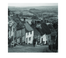
(a) Original image

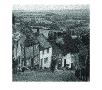
(b) Noisy image

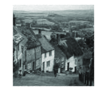
(c) Denoised using curvelets

(d) Denoised using shearlets

(e) Denoised using curvelets (zoom)

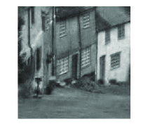
(f) Denoised using shearlets (zoom)

Figure 1: Denoising of the Goldhill image ($512\times 512$) using shearlets and curvelets. The noisy image in (b) has a peak signal-to-noise ratio of $20.17$ dB. The curvelet-denoised image in (c) and (e) has a PSNR of $28.70$ dB, while the shearlet-denoised image in (d) and (f) has a PSNR of only $29.20$ dB.

Curvelets CDDY06 .

This approach builds on directional frequency partitioning and the use of the Fast Fourier transform. The algorithm can be efficiently implemented using (in frequency domain) multiplication with the frequency response of a filter and frequency wrapping in place of convolution and down-sampling. However, curvelets need to be band-limited and can only have very good spatial localization if one allows high redundancy.

Contourlets DV05 .

This approach uses a directional filter bank, which produces directional frequency partitioning similar to those of curvelets. As the main advantage of this approach, it allows a tree-structured filter bank implementation, in which aliasing due to subsampling is allowed to exist. Consequently, one can achieve great efficiency in terms of redundancy and good spatial localization. However, the directional selectivity in this approach is artificially imposed by the special sampling rule of a filter bank which introduces various artifacts. We remark that also the recently introduced Hybrid Wavelets ER07 suffer from this deficiency.

Shearlets Lim09b .

Using a shear matrix instead of rotation, directionality is naturally adapted for the digital setting in the sense that the shear matrix preserves the structure of the integer grid. Furthermore, excellent spatial localization is achieved by using compactly supported shearlets. The only drawback is that these compactly supported shearlets are not tight frames and, accordingly, the synthesis process needs to be performed by iterative methods.

To illustrate how two of these implementations perform, we have included a denoising example of the Goldhill image using both curvelets and shearlets, see Figure 1. We omit a detailed analysis of the denoising results and leave the visual comparison to the reader. For a detailed review of the shearlet transform and associated aspects, we refer to Lim09b ; DKS08 ; ELL08 ; DKSZ10 . We also refer to KS10 ; hks10 for MRA based algorithmic approaches to the shearlet transform.

The shearlet transform, in companion with the wavelet transform, has also been applied to accomplish geometric separation of ‘point-and-curve’-like data. An artificially made example of such data can be seen in Figure 2a. For a theoretical account of these separation ideas we refer to the recent papers by Donoho and the first author DK09 ; DK10 . Here we simply display the result of the separation, see Figure 2. For real-world applications of these separation techniques we refer to the paper avignon on neurobiological imaging.

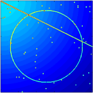
(a) Original point-curve data of size $256\times 256$.

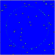
(b) Separated point-like data (captured by wavelets).

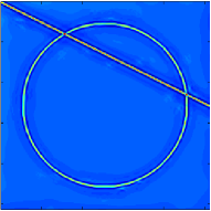
(c) Separated curve-like data (captured by shearlets).

Figure 2: Geometric separation of mixed ‘point-and-curve’ data. (a): Input data. (b) and (c): The output of the separation algorithm.

In the spirit of reproducible research DMSSU09 , we wish to mention that Figure 1d, 1f and 2 have been produced by the discrete shearlet transform implemented in the Matlab toolbox Shearlab which has recently been released under a GNU license and is freely available at http://www.shearlab.org.

1.5 Outline

In Section 2 we present a review of shearlet theory in $L^{2}(\mathbb{R}^{2})$, where we focus on discrete shearlet systems. We describe the classical band-limited construction (Section 2.2) and a more recent construction of compactly supported shearlets (Section 2.3). In Section 3 we present results on the ability of shearlets to optimally sparsely approximate cartoon-like images. Section 4 is dedicated to a discussion on similar properties of 3D shearlet systems.

2 2D Shearlets

In this section, we summarize what is known about constructions of discrete shearlet systems in 2D. Although all results in this section can easily be extended to (irregular) shearlet systems associated with a general irregular set of parameters for scaling, shear, and translation, we will only focus on the discrete shearlet systems associated with a regular set of parameters as described in the next section. For a detailed analysis of irregular shearlet systems, we refer to KLP10 . We first start with various notations and definitions for later use.

2.1 Preliminaries

For $j\geq 0,k\in\mathbb{Z}$, let

$$A_{2^{j}}=\begin{pmatrix}2^{j}&0\\ 0&2^{j/2}\end{pmatrix},\,\,S_{k}=\begin{pmatrix}1&k\\ 0&1\end{pmatrix},\quad\text{and}\quad M_{c}=\begin{pmatrix}c_{1}&0\\ 0&c_{2}\end{pmatrix},$$

where $c=(c_{1},c_{2})$ and $c_{1},c_{2}$ are some positive constants. Similarly, we define

$$\tilde{A}_{2^{j}}=\begin{pmatrix}2^{j/2}&0\\ 0&2^{j}\end{pmatrix},\,\,\tilde{S}_{k}=\begin{pmatrix}1&0\\ k&1\end{pmatrix},\quad\text{and}\quad\tilde{M}_{c}=\begin{pmatrix}c_{2}&0\\ 0&c_{1}\end{pmatrix}.$$

Next we define discrete shearlet systems in 2D.

Definition 1

Let $c=(c_{1},c_{2})\in(\mathbb{R}_{+})^{2}$. For $\phi,\psi,\tilde{\psi}\in L^{2}(\mathbb{R}^{2})$ the cone-adapted 2D discrete shearlet system $SH(\phi,\psi,\tilde{\psi};c)$ is defined by

$$SH(\phi,\psi,\tilde{\psi};c)=\Phi(\phi;c_{1})\cup\Psi(\psi;c)\cup\tilde{\Psi}(\tilde{\psi};c),$$

where

$$\Phi(\phi;c_{1}) =\{\phi(\cdot-m):m\in c_{1}\mathbb{Z}^{2}\},$$

$$\Psi(\psi;c) =\{2^{\frac{3}{4}j}\psi(S_{k}A_{2^{j}}\,\cdot\,-m):j\geq 0,-\lceil 2^{j/2}\rceil\leq k\leq\lceil 2^{j/2}\rceil,m\in M_{c}\mathbb{Z}^{2}\},$$

and

$$\tilde{\Psi}(\tilde{\psi};c) =\{2^{\frac{3}{4}j}\tilde{\psi}(\tilde{S}_{k}\tilde{A}_{2^{j}}\,\cdot\,-m):j\geq 0,-\lceil 2^{j/2}\rceil\leq k\leq\lceil 2^{j/2}\rceil,m\in\tilde{M}_{c}\mathbb{Z}^{2}\}.$$

If $SH(\phi,\psi,\tilde{\psi};c)$ is a frame for $L^{2}(\mathbb{R}^{2})$, we refer to $\phi$ as a scaling function and $\psi$ and $\tilde{\psi}$ as shearlets.

Our aim is to construct compactly supported functions $\phi,\psi$, and $\tilde{\psi}$ to obtain compactly supported shearlets in 2D. For this, we will describe general sufficient conditions on the shearlet generators $\psi$ and $\tilde{\psi}$, which lead to the construction of compactly supported shearlets. To formulate our sufficient conditions on $\psi$ and $\tilde{\psi}$ (Section 2.3), we will first need to introduce the necessary notational concepts.

For functions $\phi,\psi,\tilde{\psi}\in L^{2}(\mathbb{R}^{2})$, we define $\Theta:\mathbb{R}^{2}\times\mathbb{R}^{2}\to\mathbb{R}$ by

$$\Theta(\xi,\omega)=|\hat{\phi}(\xi)||\hat{\phi}(\xi+\omega)|+\Theta_{1}(\xi,\omega)+\Theta_{2}(\xi,\omega),$$ (1)

where

$$\Theta_{1}(\xi,\omega)=\sum\limits_{j\geq 0}\sum\limits_{|k|\leq\lceil 2^{j/2}\rceil}\left|\hat{\psi}(S_{{k}}^{T}A_{{2^{-j}}}\xi)\right|\left|\hat{\psi}({S_{k}}^{T}A_{{2^{-j}}}\xi+\omega)\right|$$

and

$$\Theta_{2}(\xi,\omega)=\sum\limits_{j\geq 0}\sum\limits_{|k|\leq\lceil 2^{j/2}\rceil}\left|\hat{\tilde{\psi}}({S}_{{k}}\tilde{A}_{{2^{-j}}}\xi)\right|\left|\hat{\tilde{\psi}}({S}_{{k}}\tilde{A}_{{2^{-j}}}\xi+\omega)\right|.$$

Also, for $c=(c_{1},c_{2})\in(\mathbb{R}_{+})^{2}$, let

$$R(c) =\sum_{m\in\mathbb{Z}^{2}\setminus\{0\}}\left(\Gamma_{0}(c_{1}^{-1}m)\Gamma_{0}(-c_{1}^{-1}m)\right)^{\frac{1}{2}}+\left(\Gamma_{1}(M_{c}^{-1}m)\Gamma_{1}(-M_{c}^{-1}m)\right)^{\frac{1}{2}}$$

$$\phantom{\sum_{m\in\mathbb{Z}^{2}\setminus\{0\}}+}+(\Gamma_{2}(\tilde{M}_{c}^{-1}m)\Gamma_{2}(-\tilde{M}_{c}^{-1}m))^{\frac{1}{2}},$$

where

$$\Gamma_{0}(\omega)=\operatorname*{ess\,sup}_{\xi\in\mathbb{R}^{2}}|\hat{\phi}(\xi)||\hat{\phi}(\xi+\omega)|\quad\text{and}\quad\Gamma_{i}(\omega)=\operatorname*{ess\,sup}_{\xi\in\mathbb{R}^{2}}\Theta_{i}(\xi,\omega)\quad\text{for}\,\,i=1,2.$$

2.2 Classical Construction

We now first describe the construction of band-limited shearlets which provides tight frames for $L^{2}(\mathbb{R}^{2})$. Constructions of this type were first introduced by Labate, Weiss, and two of the authors in LLKW05 . The classical example of a generating shearlet is a function $\psi\in L^{2}(\mathbb{R}^{2})$ satisfying

$$\hat{\psi}(\xi)=\hat{\psi}(\xi_{1},\xi_{2})=\hat{\psi}_{1}(\xi_{1})\,\hat{\psi}_{2}(\tfrac{\xi_{2}}{\xi_{1}}),$$

where $\psi_{1}\in L^{2}(\mathbb{R})$ is a discrete wavelet, i.e., satisfies the discrete Calderón condition given by

$$\sum_{j\in\mathbb{Z}}\lvert\hat{\psi}_{1}(2^{-j}\xi)\rvert^{2}=1\quad\mbox{for a.e. }\xi\in\mathbb{R},$$

with $\hat{\psi}_{1}\in C^{\infty}(\mathbb{R})$ and $\operatorname{supp}\hat{\psi}_{1}\subseteq[-\frac{5}{4},-\frac{1}{4}]\cup[\frac{1}{4},\frac{5}{4}]$, and $\psi_{2}\in L^{2}(\mathbb{R})$ is a bump function, namely

$$\sum_{k=-1}^{1}\lvert\hat{\psi}_{2}(\xi+k)\rvert^{2}=1\quad\mbox{for a.e. }\xi\in[-1,1],$$

satisfying $\hat{\psi}_{2}\in C^{\infty}(\mathbb{R})$ and $\operatorname{supp}\hat{\psi}_{2}\subseteq\left[{-1},{1}\right]$. There are several choices of $\psi_{1}$ and $\psi_{2}$ satisfying those conditions, and we refer to GKL06 for further details.

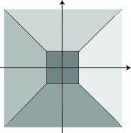
Figure 3: The cones ${\mathcal{C}}_{1}$ – ${\mathcal{C}}_{4}$ and the centered rectangle ${\mathcal{R}}$ in the frequency domain.

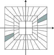
Figure 4: Tiling of the frequency domain induced by band-limited shearlets.

The tiling of the frequency domain given by these band-limited generators and choosing $\tilde{\psi}(x_{1},x_{2})=\psi(x_{2},x_{1})$ is illustrated in Figure 4. As described in Figure 4, a conic region ${\mathcal{C}}_{1}\cup{\mathcal{C}}_{3}$ is covered by the frequency support of shearlets in $\Psi(\psi;c)$ while ${\mathcal{C}}_{2}\cup{\mathcal{C}}_{4}$ is covered by $\tilde{\Psi}(\tilde{\psi};c)$. For this particular choice, using an appropriate scaling function $\phi$ for the centered rectangle ${\mathcal{R}}$ (see Figure 4), it was proved in (GKL06, , Thm. 3) that the associated cone-adapted discrete shearlet system $SH(\phi,\psi,\tilde{\psi};(1,1))$ forms a Parseval frame for $L^{2}(\mathbb{R}^{2})$.

2.3 Constructing Compactly Supported Shearlets

We are now ready to state general sufficient conditions for the construction of shearlet frames.

Theorem 2.1 (KLP10 )

Let $\phi,\psi\in L^{2}(\mathbb{R}^{2})$ be functions such that

$$\hat{\phi}(\xi_{1},\xi_{2})\leq C_{1}\cdot\min{\{1,\left\lvert\xi_{1}\right\rvert^{-\gamma}\}}\cdot\min{\{1,|\xi_{2}|^{-\gamma}\}}$$

and

$$\left\lvert\hat{\psi}(\xi_{1},\xi_{2})\right\rvert\leq C_{2}\cdot\min\{1,|\xi_{1}|^{\alpha}\}\cdot\min{\{1,|\xi_{1}|^{-\gamma}\}}\cdot\min{\{1,|\xi_{2}|^{-\gamma}\}},$$ (2)

for some positive constants $C_{1},C_{2}<\infty$ and $\alpha>\gamma>3$. Define $\tilde{\psi}(x_{1},x_{2})=\psi(x_{2},x_{1})$, and let $L_{\inf},L_{\sup}$ be defined by

$$L_{\inf}=\operatorname*{ess\,inf}\limits_{\xi\in\mathbb{R}^{2}}\Theta(\xi,0)\quad\text{and}\quad L_{\sup}=\operatorname*{ess\,sup}\limits_{\xi\in\mathbb{R}^{2}}\Theta(\xi,0).$$

Suppose that there is a constant $\tilde{L}_{\inf}>0$ such that $0<\tilde{L}_{\inf}\leq L_{\inf}$. Then there exist a sampling parameter $c=(c_{1},c_{2})$ with $c_{1}=c_{2}$ and a constant $\tilde{L}_{sup}<\infty$ such that

$$R(c)<\tilde{L}_{inf}\leq L_{inf}\,\,\mbox{and}\,\,L_{sup}\leq\tilde{L}_{sup},$$

and, further, ${SH}(\phi,\psi,\tilde{\psi};c)$ forms a frame for $L^{2}(\mathbb{R}^{2})$ with frame bounds $A$ and $B$ satisfying

$$\frac{1}{|\det M_{c}|}[\tilde{L}_{inf}-R(c)]\leq A\leq B\leq\frac{1}{|\det M_{c}|}[\tilde{L}_{sup}+R(c)].$$ (3)

For a detailed proof, we refer to the paper KLP10 by Kittipoom and two of the authors.

Obviously, band-limited shearlets (from Section 2.2) satisfy condition (2). More interestingly, also a large class of spatially compactly supported functions satisfies this condition. In fact, in KLP10 , various constructions of compactly supported shearlets are presented using Theorem 2.1 and generalized low-pass filters; an example of such a construction procedure is given in Theorem 2.2 below. In Theorem 2.1 we assumed $c_{1}=c_{2}$ for the sampling matrix $M_{c}$ (or $\tilde{M}_{c}$), the only reason for this being the simplification of the estimates for the frame bounds $A,B$ in (3). In fact, the estimate (3) generalizes easily to non-uniform sampling constants $c_{1},c_{2}$ with $c_{1}\neq c_{2}$. For explicit estimates of the form (3) in the case of non-uniform sampling, we refer to KLP10 .

The following result provides a specific family of functions satisfying the general sufficiency condition from Theorem 2.1.

Theorem 2.2 ( KLP10 )

Let $K,L>0$ be such that $L\geq 10$ and $\frac{3L}{2}\leq K\leq 3L-2$, and define a shearlet $\psi\in L^{2}(\mathbb{R}^{2})$ by

$$\hat{\psi}(\xi)=m_{1}(4\xi_{1})\hat{\phi}(\xi_{1})\hat{\phi}(2\xi_{2}),\quad\xi=(\xi_{1},\xi_{2})\in\mathbb{R}^{2},$$

where $m_{0}$ is the low pass filter satisfying

$$|m_{0}(\xi_{1})|^{2}=(\cos(\pi\xi_{1}))^{2K}\sum_{n=0}^{L-1}\binom{K-1+n}{n}(\sin(\pi\xi_{1}))^{2n},\quad\xi_{1}\in\mathbb{R},$$

$m_{1}$ is the associated bandpass filter defined by

$$|m_{1}(\xi_{1})|^{2}=|m_{0}(\xi_{1}+\tfrac{1}{2})|^{2},\quad\xi_{1}\in\mathbb{R},$$

and $\phi$ is the scaling function given by

$$\hat{\phi}(\xi_{1})=\prod_{j=0}^{\infty}m_{0}(2^{-j}\xi_{1}),\quad\xi_{1}\in\mathbb{R}.$$

Then there exists a sampling constant $\hat{c}_{1}>0$ such that the shearlet system $\Psi(\psi;c)$ forms a frame for $\check{L}^{2}({\mathcal{C}}_{1}\cup{\mathcal{C}}_{3}):=\left\{{f\in L^{2}(\mathbb{R}^{2})}:{\operatorname{supp}\hat{f}\subset{\mathcal{C}}_{1}\cup{\mathcal{C}}_{3}}\right\}$ for any sampling matrix $M_{c}$ with $c=(c_{1},c_{2})\in(\mathbb{R}_{+})^{2}$ and $c_{2}\leq c_{1}\leq\hat{c}_{1}$.

For these shearlet systems, there is a bias towards the vertical axis, especially at coarse scales, since they are defined for $\check{L}^{2}({\mathcal{C}}_{1}\cup{\mathcal{C}}_{3})$, and hence, the frequency support of the shearlet elements overlaps more significantly along the vertical axis. In order to control the upper frame bound, it is therefore desirable to apply a denser sampling along the vertical axis than along the horizontal axis, i.e., $c_{1}>c_{2}$.

Having compactly supported (separable) shearlet frames for $\check{L}^{2}({\mathcal{C}}_{1}\cup{\mathcal{C}}_{3})$ at hand by Theorem 2.2, we can easily construct shearlet frames for the whole space $L^{2}(\mathbb{R}^{2})$. The exact procedure is described in the following theorem from KLP10 .

Theorem 2.3 (KLP10 )

Let $\psi\in L^{2}(\mathbb{R}^{2})$ be the shearlet with associated scaling function $\phi_{1}\in L^{2}(\mathbb{R})$ both introduced in Theorem 2.2, and set $\phi(x_{1},x_{2})=\phi_{1}(x_{1})\phi_{1}(x_{2})$ and $\tilde{\psi}(x_{1},x_{2})=\psi(x_{2},x_{1})$. Then the corresponding shearlet system $SH(\phi,\psi,\tilde{\psi};c)$ forms a frame for $L^{2}(\mathbb{R}^{2})$ for any sampling matrices $M_{c}$ and $\tilde{M}_{c}$ with $c=(c_{1},c_{2})\in(\mathbb{R}_{+})^{2}$ and $c_{2}\leq c_{1}\leq\hat{c}_{1}$.

For the horizontal cone ${\mathcal{C}}_{1}\cup{\mathcal{C}}_{3}$ we allow for a denser sampling by $M_{c}$ along the vertical axis, i.e., $c_{2}\leq c_{1}$, precisely as in Theorem 2.2. For the vertical cone ${\mathcal{C}}_{2}\cup{\mathcal{C}}_{4}$ we analogously allow for a denser sampling along the horizontal axis; since the position of $c_{1}$ and $c_{2}$ is reversed in $\tilde{M}_{c}$ compared to $M_{c}$, this still corresponds to $c_{2}\leq c_{1}$.

We wish to mention that there is a trade-off between compact support of the shearlet generators, tightness of the associated frame, and separability of the shearlet generators. The known constructions of tight shearlet frames do not use separable generators (Section 2.2), and these constructions can be shown to not be applicable to compactly supported generators. Tightness is difficult to obtain while allowing for compactly supported generators, but we can gain separability as in Theorem 2.3, hence fast algorithmic realizations. On the other hand, when allowing non-compactly supported generators, tightness is possible, but separability seems to be out of reach, which makes fast algorithmic realizations very difficult.

We end this section by remarking that the construction results above even generalize to constructions of irregular shearlet systems KL07 ; KKL10 .

3 Sparse Approximations

After having introduced compactly supported shearlet systems in the previous section, we now aim for optimally sparse approximations. To be precise, we will show that these compactly supported shearlet systems provide optimally sparse approximations when representing and analyzing anisotropic features in 2D data.

3.1 Cartoon-Like Image Model

Following Don01 , we introduce $STAR^{2}(\nu)$, a class of sets $B$ with $C^{2}$ boundaries $\partial B$ and curvature bounded by $\nu$, as well as ${\mathcal{E}}^{2}_{\nu}(\mathbb{R}^{2})$, a class of cartoon-like images. For this, in polar coordinates, we let $\rho:\left[{0},{2\pi}\right)\rightarrow[0,1]$ be a radius function and define the set $B$ by

$$B=\{x\in\mathbb{R}^{2}:\left\lvert x\right\rvert\leq\rho(\theta),\,x=(\left\lvert x\right\rvert,\theta)\text{ in polar coordinates}\}.$$

In particular, we will require that the boundary $\partial B$ of $B$ is given by the curve

$$\beta(\theta)=\begin{pmatrix}\rho(\theta)\cos(\theta)\\ \rho(\theta)\sin(\theta)\end{pmatrix},$$ (4)

and the class of boundaries of interest to us are defined by

$$\sup\lvert\rho^{{}^{\prime\prime}}(\theta)\rvert\leq\nu,\quad\rho\leq\rho_{0}<1,$$ (5)

where $\rho_{0}<1$ needs to be chosen so that $y+B\subset\left[{0},{1}\right]^{2}$ for some $y\in\mathbb{R}^{2}$.

The following definition now introduces a class of cartoon-like images.

Definition 2

For $\nu>0$, the set $STAR^{2}(\nu)$ is defined to be the set of all $B\subset[0,1]^{2}$ such that $B$ is a translate of a set obeying (4) and (5). Further, ${\mathcal{E}}^{2}_{\nu}(\mathbb{R}^{2})$ denotes the set of functions $f\in L^{2}(\mathbb{R}^{2})$ of the form

$$f=f_{0}+f_{1}\chi_{B},$$

where $B\in STAR^{2}(\nu)$ and $f_{0},f_{1}\in C_{0}^{2}(\mathbb{R}^{2})$ with $\operatorname{supp}f_{i}\subset\left[{0},{1}\right]^{2}$ and $\|f_{i}\|_{C^{2}}=\sum_{|\alpha|\leq 2}\|D^{\alpha}f_{i}\|_{\infty}\leq 1$ for $i=1,2$.

One can also consider a more sophisticated class of cartoon-like images, where the boundary of $B$ is allowed to be piecewise $C^{2}$, and we refer to the recent paper by two of the authors KL10SoBD and to similar considerations for the 3D case in Section 4.2.

Donoho Don01 proved that the optimal approximation rate for such cartoon-like image models $f\in{\mathcal{E}}^{2}_{\nu}(\mathbb{R}^{2})$ which can be achieved for almost any representation system under a so-called polynomial depth search selection procedure of the selected system elements is

$$\left\lVert f-f_{N}\right\rVert_{2}^{2}\leq C\cdot N^{-2}\quad\text{as }N\to\infty,$$

where $f_{N}$ is the best $N$-term approximation of $f$. As discussed in the next section shearlets in 2D do indeed deliver this optimal approximation rate.

3.2 Optimally Sparse Approximation of Cartoon-Like Images

Let $SH(\phi,\psi,\tilde{\psi};c)$ be a shearlet frame for $L^{2}(\mathbb{R}^{2})$. Since this is a countable set of functions, we can denote it by $SH(\phi,\psi,\tilde{\psi};c)=(\sigma_{i})_{i\in I}$. We let $(\tilde{\sigma}_{i})_{i\in I}$ be a dual frame of $(\sigma_{i})_{i\in I}$. As our $N$-term approximation $f_{N}$ of a cartoon-like image $f\in{\mathcal{E}}^{2}_{\nu}(\mathbb{R}^{2})$ by the frame $SH(\phi,\psi,\tilde{\psi};c)$, we then take

$$f_{N}=\sum_{i\in I_{N}}\left\langle f,\sigma_{i}\right\rangle_{\!}\tilde{\sigma}_{i},$$

where $(\left\langle f,\sigma_{i}\right\rangle_{\!})_{i\in I_{N}}$ are the $N$ largest coefficients $\left\langle f,\sigma_{i}\right\rangle_{\!}$ in magnitude. As in the tight frame case, this procedure does not always yield the best $N$-term approximation, but, surprisingly, even with this rather crude selection procedure, we can prove an (almost) optimally sparse approximation rate. We speak of ‘almost’ optimality due to the (negligible) $\log$-factor in (6). The following result shows that our ‘new’ compactly supported shearlets (see Section 2.3) deliver the same approximation rate as band-limited curvelets CD04 , contourlets DV05 , and shearlets GL07 .

Theorem 3.1 (KL10 )

Let $c>0$, and let $\phi,\psi,\tilde{\psi}\in L^{2}(\mathbb{R}^{2})$ be compactly supported. Suppose that, in addition, for all $\xi=(\xi_{1},\xi_{2})\in\mathbb{R}^{2}$, the shearlet $\psi$ satisfies

1. $|\hat{\psi}(\xi)|\leq C_{1}\cdot\min\{1,|\xi_{1}|^{\alpha}\}\cdot\min\{1,|\xi_{1}|^{-\gamma}\}\cdot\min\{1,|\xi_{2}|^{-\gamma}\}$        and

2. $\left|\frac{\partial}{\partial\xi_{2}}\hat{\psi}(\xi)\right|\leq|h(\xi_{1})|\cdot\left(1+\frac{|\xi_{2}|}{|\xi_{1}|}\right)^{-\gamma}$,

where $\alpha>5$, $\gamma\geq 4$, $h\in L^{1}(\mathbb{R})$, and $C_{1}$ is a constant, and suppose that the shearlet $\tilde{\psi}$ satisfies (i) and (ii) with the roles of $\xi_{1}$ and $\xi_{2}$ reversed. Further, suppose that $SH(\phi,\psi,\tilde{\psi};c)$ forms a frame for $L^{2}(\mathbb{R}^{2})$.

Then, for any $\nu>0$, the shearlet frame $SH(\phi,\psi,\tilde{\psi};c)$ provides (almost) optimally sparse approximations of functions $f\in{\mathcal{E}}^{2}_{\nu}(\mathbb{R}^{2})$ in the sense that there exists some $C>0$ such that

$$\|f-f_{N}\|_{2}^{2}\leq C\cdot N^{-2}\cdot{(\log{N})}^{3}\qquad\text{as }N\rightarrow\infty,$$ (6)

where $f_{N}$ is the nonlinear N-term approximation obtained by choosing the N largest shearlet coefficients of $f$.

Condition (i) can be interpreted as both a condition ensuring (almost) separable behavior as well as a moment condition along the horizontal axis, hence enforcing directional selectivity. This condition ensures that the support of shearlets in frequency domain is essentially of the form indicated in Figure 4. Condition (ii) (together with (i)) is a weak version of a directional vanishing moment condition, which is crucial for having fast decay of the shearlet coefficients when the corresponding shearlet intersects the discontinuity curve. Conditions (i) and (ii) are rather mild conditions on the generators; in particular, shearlets constructed by Theorem 2.2 and 2.3, with extra assumptions on the parameters $K$ and $L$, will indeed satisfy (i) and (ii) in Theorem 3.1. To compare with the optimality result for band-limited generators we wish to point out that conditions (i) and (ii) are obviously satisfied for band-limited generators.

We remark that this kind of approximation result is not available for shearlet systems coming directly from the shearlet group. One reason for this being that these systems, as mentioned several times, do not treat directions in a uniform way.

4 Shearlets in 3D and Beyond

Shearlet theory has traditionally only dealt with representation systems for two-dimensional data. In the recent paper DST09 (and the accompanying paper DT10 ) this was changed when Dahlke, Steidl, and Teschke generalized the continuous shearlet transform (see KL09 ; DKMSST08 ) to higher dimensions. The shearlet transform on $L^{2}(\mathbb{R}^{n})$ by Dahlke, Steidl, and Teschke is associated with the so-called shearlet group in $\mathbb{R}\setminus\{0\}\times\mathbb{R}^{n-1}\times\mathbb{R}^{n}$, with a dilation matrix of the form

$$A_{a}=\operatorname{diag}{(a,\mathrm{sgn}(a)\left\lvert a\right\rvert^{1/n},\dots,\mathrm{sgn}(a)\left\lvert a\right\rvert^{1/n})},\qquad a\in\mathbb{R}\setminus\{0\},$$

and with a shearing matrix with $n-1$ shear parameters $s=(s_{1},\dots,s_{n-1})\in\mathbb{R}^{n-1}$ of the form

$$S_{s}=\begin{bmatrix}1&s\\ 0&I_{n-1}\end{bmatrix},$$

where $I_{n}$ denotes the $n\times n$ identity matrix. This type of shearing matrix gives rise to shearlets consisting of wedges of size $a^{-1}\times a^{-1/n}\times\dots\times a^{-1/n}$ in frequency domain, where $a^{-1}\gg a^{-1/n}$ for small $a>0$. Hence, for small $a>0$, the spatial appearance is a surface-like element of co-dimension one.

In the following section we will consider shearlet systems in $L^{2}(\mathbb{R}^{3})$ associated with a sightly different shearing matrix. More importantly, we will consider pyramid-adapted 3D shearlet systems, since these systems treat directions in a uniform way as opposed to the shearlet systems coming from the shearlet group; this design, of course, parallels the idea behind cone-adapted 2D shearlets. In GL10 , the continuous version of the pyramid-adapted shearlet system was introduced, and it was shown that the location and the local orientation of the boundary set of certain three-dimensional solid regions can be precisely identified by this continuous shearlet transform. The pyramid-adapted shearlet system can easily be generalized to higher dimensions, but for brevity we only consider the three-dimensional setup and newly introduce it now in the discrete setting.

4.1 Pyramid-Adapted Shearlet Systems

We will scale according to paraboloidal scaling matrices $A_{2^{j}}$, $\tilde{A}_{2^{j}}$ or $\breve{A}_{2^{j}}$, $j\in\mathbb{Z}$, and encode directionality by the shear matrices $S_{k}$, $\tilde{S}_{k}$, or $\breve{S}_{k}$, $k=(k_{1},k_{2})\in\mathbb{Z}^{2}$, defined by

$$A_{2^{j}} =\begin{pmatrix}2^{j}&0&0\\ 0&2^{j/2}&0\\ 0&0&2^{j/2}\end{pmatrix}, \tilde{A}_{2^{j}} = \begin{pmatrix}2^{j/2}&0&0\\ 0&2^{j}&0\\ 0&0&2^{j/2}\end{pmatrix}, \breve{A}_{2^{j}} = \begin{pmatrix}2^{j/2}&0&0\\ 0&2^{j/2}&0\\ 0&0&2^{j}\end{pmatrix},$$ and

and

$$S_{k} =\begin{pmatrix}1\;&k_{1}\;&k_{2}\\ 0&1&0\\ 0&0&1\end{pmatrix}, \tilde{S}_{k} = \begin{pmatrix}1&0&0\\ k_{1}\;&1\;&k_{2}\\ 0&0&1\end{pmatrix}, \breve{S}_{k}\; = \begin{pmatrix}1&0&0\\ 0&1&0\\ k_{1}\;&k_{2}\;&1\end{pmatrix},$$ and

respectively. The translation lattices will be defined through the following matrices: $M_{c}=\mathrm{diag}(c_{1},c_{2},c_{2})$, $\tilde{M}_{c}=\mathrm{diag}(c_{2},c_{1},c_{2})$, and $\breve{M}_{c}=\mathrm{diag}(c_{2},c_{2},c_{1})$, where $c_{1}>0$ and $c_{2}>0$.

t]

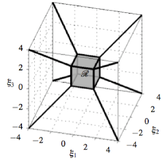
Figure 5: The partition of the frequency domain: The centered rectangle ${\mathcal{R}}$. The arrangement of the six pyramids is indicated by the ‘diagonal’ lines. See Figure 6 for a sketch of the pyramids.

We next partition the frequency domain into the following six pyramids:

$${\mathcal{P}}_{\iota}=\left\{\begin{array}[]{rcl}\{(\xi_{1},\xi_{2},\xi_{3})\in\mathbb{R}^{3}:\xi_{1}\geq 1,\,|\xi_{2}/\xi_{1}|\leq 1,\,|\xi_{3}/\xi_{1}|\leq 1\}&:&\iota=1,\\ \{(\xi_{1},\xi_{2},\xi_{3})\in\mathbb{R}^{3}:\xi_{2}\geq 1,\,|\xi_{1}/\xi_{2}|\leq 1,\,|\xi_{3}/\xi_{2}|\leq 1\}&:&\iota=2,\\ \{(\xi_{1},\xi_{2},\xi_{3})\in\mathbb{R}^{3}:\xi_{3}\geq 1,\,|\xi_{1}/\xi_{3}|\leq 1,\,|\xi_{2}/\xi_{3}|\leq 1\}&:&\iota=3,\\ \{(\xi_{1},\xi_{2},\xi_{3})\in\mathbb{R}^{3}:\xi_{1}\leq-1,\,|\xi_{2}/\xi_{1}|\leq 1,\,|\xi_{3}/\xi_{1}|\leq 1\}&:&\iota=4,\\ \{(\xi_{1},\xi_{2},\xi_{3})\in\mathbb{R}^{3}:\xi_{2}\leq-1,\,|\xi_{1}/\xi_{2}|\leq 1,\,|\xi_{3}/\xi_{2}|\leq 1\}&:&\iota=5,\\ \{(\xi_{1},\xi_{2},\xi_{3})\in\mathbb{R}^{3}:\xi_{3}\leq-1,\,|\xi_{1}/\xi_{3}|\leq 1,\,|\xi_{2}/\xi_{3}|\leq 1\}&:&\iota=6,\end{array}\right.$$

and a centered rectangle

$${\mathcal{R}}=\{(\xi_{1},\xi_{2},\xi_{3})\in\mathbb{R}^{3}:\left\lVert(\xi_{1},\xi_{2},\xi_{3})\right\rVert_{\infty}<1\}.$$

The partition is illustrated in Figures 5 and 6. This partition of the frequency space allows us to restrict the range of the shear parameters. In the case of ‘shearlet group’ systems one must allow arbitrarily large shear parameters, while the ‘pyramid-adapted’ systems restrict the shear parameters to $\left[{-\lceil 2^{j/2}\rceil},{\lceil 2^{j/2}\rceil}\right]$. It is exactly this fact that gives a more uniform treatment of the directionality properties of the shearlet system.

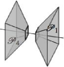
(a) Pyramids ${\mathcal{P}}_{1}$ and ${\mathcal{P}}_{4}$ and the $\xi_{1}$ axis.

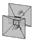
(b) Pyramids ${\mathcal{P}}_{2}$ and ${\mathcal{P}}_{5}$ and the $\xi_{2}$ axis.

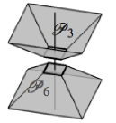
(c) Pyramids ${\mathcal{P}}_{3}$ and ${\mathcal{P}}_{6}$ and the $\xi_{3}$ axis.

Figure 6: The partition of the frequency domain: The ‘top’ of the six pyramids.

These considerations are now made precise in the following definition.

Definition 3

For $c=(c_{1},c_{2})\in(\mathbb{R}_{+})^{2}$, the pyramid-adapted 3D shearlet system $SH(\phi,\psi,\tilde{\psi},\breve{\psi};c)$ generated by $\phi,\psi,\tilde{\psi},\breve{\psi}\in L^{2}(\mathbb{R}^{3})$ is defined by

$$SH(\phi,\psi,\tilde{\psi},\breve{\psi};c)=\Phi(\phi;c_{1})\cup\Psi(\psi;c)\cup\tilde{\Psi}(\tilde{\psi};c)\cup\breve{\Psi}(\breve{\psi};c),$$

where

$$\Phi(\phi;c_{1}) =\left\{{\phi_{m}=\phi(\cdot-m)}:{m\in c_{1}\mathbb{Z}^{3}}\right\},$$

$$\Psi(\psi;c) =\left\{{\psi_{j,k,m}=2^{j}{\psi}({S}_{k}{A}_{2^{j}}\cdot-m)}:{j\geq 0,|k|\leq\lceil 2^{j/2}\rceil,m\in M_{c}\mathbb{Z}^{3}}\right\},$$

$$\tilde{\Psi}(\tilde{\psi};c) =\{\tilde{\psi}_{j,k,m}=2^{j}\tilde{\psi}(\tilde{S}_{k}\tilde{A}_{2^{j}}\cdot-m):j\geq 0,|k|\leq\lceil 2^{j/2}\rceil,m\in\tilde{M}_{c}\mathbb{Z}^{3}\},$$

and

$$\breve{\Psi}(\breve{\psi};c) =\{\breve{\psi}_{j,k,m}=2^{j}\breve{\psi}(\breve{S}_{k}\breve{A}_{2^{j}}\cdot-m):j\geq 0,|k|\leq\lceil 2^{j/2}\rceil,m\in\breve{M}_{c}\mathbb{Z}^{3}\},$$

where $j\in\mathbb{N}_{0}$ and $k\in\mathbb{Z}^{2}$. Here we have used the vector notation $\left\lvert k\right\rvert\leq K$ for $k=(k_{1},k_{2})$ and $K>0$ to denote $\left\lvert k_{1}\right\rvert\leq K$ and $\left\lvert k_{2}\right\rvert\leq K$.

The construction of pyramid-adapted shearlet systems $SH(\phi,\psi,\tilde{\psi},\breve{\psi};c)$ runs along the lines of the construction of cone-adapted shearlet systems in $L^{2}(\mathbb{R}^{2})$ described in Section 2.3. For a detailed description, we refer to KLL10 .

We remark that the shearlets in spatial domain are of size $2^{-j/2}$ times $2^{-j/2}$ times $2^{-j}$ which shows that the shearlet elements will become ‘plate-like’ as $j\to\infty$. One could also use the scaling matrix $A_{2^{j}}=\operatorname{diag}{(2^{j},2^{j},2^{j/2})}$ with similar changes for $\tilde{A}_{2^{j}}$ and $\breve{A}_{2^{j}}$. This would lead to ‘needle-like’ shearlet elements instead of the ‘plate-like’ elements considered in this paper, but we will not pursue this further here, and simply refer to KLL10 . More generally, it is possible to even consider non-paraboloidal scaling matrices of the form $A_{j}=\operatorname{diag}{(2^{j},2^{\alpha j},2^{\beta j})}$ for $0<\alpha,\beta\leq 1$. One drawback of allowing such general scaling matrices is the lack of fast algorithms for non-dyadic multiscale systems. On the other hand, the parameters $\alpha$ and $\beta$ allow us to precisely shape the shearlet elements, ranging from very plate-like to very needle-like, according to the application at hand, i.e., choosing the shearlet-shape that is the best ‘fit’ for the geometric characteristics of the considered data.

4.2 Sparse Approximations of 3D Data

We now consider approximations of three-dimensional cartoon-like images using shearlets introduced in the previous section. The three-dimensional cartoon-like images ${\mathcal{E}}^{2}_{\nu}(\mathbb{R}^{3})$ will be piecewise $C^{2}$ functions with discontinuities on a closed $C^{2}$ surface whose principal curvatures are bounded by $\nu$. In KLL10 it was shown that the optimal approximation rate for such 3D cartoon-like image models $f\in{\mathcal{E}}^{2}_{\nu}(\mathbb{R}^{3})$ which can be achieved for almost any representation system (under polynomial depth search selection procedure of the approximating coefficients) is

$$\left\lVert f-f_{N}\right\rVert_{2}^{2}\leq C\cdot N^{-1}\quad\text{as }N\to\infty,$$

where $f_{N}$ is the best $N$-term approximation of $f$. The following result shows that compactly supported pyramid-adapted shearlets do (almost) deliver this approximation rate.

Theorem 4.1 (KLL10 )

Let $c\in(\mathbb{R}_{+})^{2}$, and let $\phi,\psi,\tilde{\psi},\breve{\psi}\in L^{2}(\mathbb{R}^{3})$ be compactly supported. Suppose that, for all $\xi=(\xi_{1},\xi_{2},\xi_{3})\in\mathbb{R}^{3}$, the function $\psi$ satisfies:

1. $|\hat{\psi}(\xi)|\leq C_{1}\cdot\min\{1,|\xi_{1}|^{\alpha}\}\cdot\min\{1,|\xi_{1}|^{-\gamma}\}\cdot\min\{1,|\xi_{2}|^{-\gamma}\}\cdot\min\{1,|\xi_{3}|^{-\gamma}\}$,

2. $\left|\frac{\partial}{\partial\xi_{i}}\hat{\psi}(\xi)\right|\leq|h(\xi_{1})|\cdot\left(1+\frac{|\xi_{2}|}{|\xi_{1}|}\right)^{-\gamma}\left(1+\frac{|\xi_{3}|}{|\xi_{1}|}\right)^{-\gamma},\qquad i=2,3$,

where $\alpha>8$, $\gamma\geq 4$, $t\mapsto th(t)\in L^{1}(\mathbb{R})$, and $C_{1}$ a constant, and suppose that $\tilde{\psi}$ and $\breve{\psi}$ satisfy analogous conditions with the obvious change of coordinates. Further, suppose that the shearlet system $SH(\phi,\psi,\tilde{\psi},\breve{\psi};c)$ forms a frame for $L^{2}(\mathbb{R}^{3})$.

Then, for any $\nu>0$, the shearlet frame $SH(\phi,\psi,\tilde{\psi},\breve{\psi};c)$ provides (almost) optimally sparse approximations of functions $f\in{\mathcal{E}}^{2}_{\nu}(\mathbb{R}^{3})$ in the sense that there exists some $C>0$ such that

$$\|f-f_{N}\|_{2}^{2}\leq C\cdot N^{-1}\cdot{(\log{N})}^{2}\qquad\text{as }N\rightarrow\infty.$$ (7)

In the following we will give a sketch of the proof of Theorem 4.1 and, in particular, give a heuristic argument (inspired by a similar one for 2D curvelets in CD04 ) to explain the exponent $N^{-1}$ in (7).

Proof (Theorem 4.1, Sketch)

Let $f\in{\mathcal{E}}^{2}_{\nu}(\mathbb{R}^{3})$ be a 3D cartoon-like image. The main concern is to derive appropriate estimates for the shearlet coefficients $\left\langle f,\psi_{j,k,m}\right\rangle_{\!}$. We first observe that we can assume the scaling index $j$ to be sufficiently large, since $f$ as well as all shearlet elements are compactly supported and since a finite number does not contribute to the asymptotic estimate we are aiming for. In particular, this implies that we do not need to take frame elements from the ‘scaling’ system $\Phi(\phi;c_{1})$ into account. Also, we are allowed to restrict our analysis to shearlets $\psi_{j,k,m}$, since the frame elements $\tilde{\psi}_{j,k,m}$ and $\breve{\psi}_{j,k,m}$ can be handled in a similar way.

Letting $|\theta(f)|_{n}$ denote the $n$th largest shearlet coefficient $\left\langle f,\psi_{j,k,m}\right\rangle_{\!}$ in absolute value and using the frame property of $SH(\phi,\psi,\tilde{\psi},\breve{\psi};c)$, we conclude that

$$\|f-f_{N}\|_{2}^{2}\leq\frac{1}{A}\sum_{n>N}|\theta(f)|_{n}^{2},$$

for any positive integer $N$, where $A$ denotes the lower frame bound of the shearlet frame $SH(\phi,\psi,\tilde{\psi},\breve{\psi};c)$. Thus, for completing the proof, it therefore suffices to show that

$$\sum_{n>N}|\theta(f)|_{n}^{2}\leq C\cdot N^{-1}\cdot{(\log{N})}^{2}\qquad\text{as}\,\,N\rightarrow\infty.$$ (8)

For the following heuristic argument, we need to make some simplifications. We will assume to have a shearlet of the form $\psi(x)=\eta(x_{1})\varphi(x_{2})\varphi(x_{3})$, where $\eta$ is a wavelet and $\varphi$ a bump (or a scaling) function. Note that the wavelet ‘points’ in the short direction of the plate-like shearlet. We now consider three cases of coefficients $\left\langle f,\psi_{j,k,m}\right\rangle_{\!}$:

1. Shearlets $\psi_{j,k,m}$ whose support does not overlap with the boundary $\partial B$.

2. Shearlets $\psi_{j,k,m}$ whose support overlaps with $\partial B$ and is nearly tangent.

3. Shearlets $\psi_{j,k,m}$ whose support overlaps with $\partial B$, but not tangentially.

(a) Sketch of shearlets whose support does not overlap with $\partial B$.

(b) Sketch of shearlets whose support overlaps with $\partial B$ and is nearly tangent.

(c) Sketch of shearlets whose support overlaps with $\partial B$, but not tangentially.

Figure 7: The three types of shearlet $\psi_{j,k,m}$ and boundary $\partial B$ interactions considered in the heuristic argument (explaining the approximation rate $N^{-1}$). Note that only a section of $\partial B$ is shown.

As we argue in the following, only coefficients from case (b) will be significant. Case (b) is – loosely speaking – the situation in which the wavelet $\eta$ breaches, in an almost normal direction, through the discontinuity surface; as is well known from wavelet theory, 1D wavelets efficiently handle such a ‘jump’ discontinuity.

Case (a). Since $f$ is $C^{2}$ smooth away from $\partial B$, the coefficients $|\left\langle f,\psi_{j,k,m}\right\rangle_{\!}|$ will be sufficiently small owing to the wavelet $\eta$ (and the fast decay of wavelet coefficients of smooth functions).

Case (b). At scale $j>0$, there are at most $O(2^{j})$ coefficients, since the plate-like elements are of size $2^{-j/2}$ times $2^{-j/2}$ (and ‘thickness’ $2^{-j}$). By assumptions on $f$ and the support size of $\psi_{j,k,m}$, we obtain the estimate

$$|\left\langle f,\psi_{j,k,m}\right\rangle_{\!}|\leq\left\lVert f\right\rVert_{\infty}\left\lVert\psi_{j,k,m}\right\rVert_{1}\leq C_{1}\,(2^{-2j})^{1/2}\left\lVert\psi_{j,k,m}\right\rVert_{2}^{1/2}\leq C_{2}\cdot 2^{-j}$$

for some constants $C_{1},C_{2}>0$. In other words, we have $O(2^{j})$ coefficients bounded by $C_{2}\cdot 2^{-j}$. Assuming the case (a) and (c) coefficients are negligible, the $n$th largest coefficient $|\theta(f)|_{n}$ is then bounded by

$$|\theta(f)|_{n}\leq C\cdot n^{-1}.$$

Therefore,

$$\sum_{n>N}|\theta(f)|_{n}^{2}\leq\sum_{n>N}C\cdot n^{-2}\leq C\cdot\int_{N}^{\infty}x^{-2}dx\leq C\cdot N^{-1}$$

and we arrive at (8), but without the $\log$-factor. This in turn shows (7), at least heuristically, and still without the $\log$-factor.

Case (c). Finally, when the shearlets are sheared away from the tangent position in case (b), they will again be small. This is due to the vanishing moment conditions in condition (i) and (ii). ∎

Clearly, Theorem 4.1 is an ‘obvious’ three-dimensional version of Theorem 3.1. However, as opposed to the two-dimensional setting, anisotropic structures in three-dimensional data comprise of two morphologically different types of structure, namely surfaces and curves. It would therefore be desirable to allow our 3D image class to also contain cartoon-like images with curve singularities. On the other hand, the pyramid-adapted shearlets introduced in Section 4.1 are plate-like and thus, a priori, not optimal for capturing such one-dimensional singularities. Surprisingly, these plate-like shearlet systems still deliver the optimal rate $N^{-1}$ for three-dimensional cartoon-like images ${\mathcal{E}}^{2}_{\nu,L}(\mathbb{R}^{3})$, where $L$ indicates that we allow our discontinuity surface $\partial B$ to be piecewise $C^{2}$ smooth; $L\in\mathbb{N}$ is the maximal number of $C^{2}$ pieces and $\nu>0$ is an upper estimate for the principal curvatures on each piece. In other words, for any $\nu>0$ and $L\in\mathbb{N}$, the shearlet frame $SH(\phi,\psi,\tilde{\psi},\breve{\psi};c)$ provides (almost) optimally sparse approximations of functions $f\in{\mathcal{E}}^{2}_{\nu,L}(\mathbb{R}^{3})$ in the sense that there exists some $C>0$ such that

$$\|f-f_{N}\|_{2}^{2}\leq C\cdot N^{-1}\cdot{(\log{N})}^{2}\qquad\text{as }N\rightarrow\infty.$$ (9)

The conditions on the shearlets $\psi,\tilde{\psi},\breve{\psi}$ are similar to these in Theorem 4.1, but more technical, and we refer to KLL10 for the precise statements and definitions as well as the proof of the optimal approximation error rate. Here we simply remark that there exist numerous examples of shearlets $\psi,\tilde{\psi}$, and $\breve{\psi}$ satisfying these conditions, which lead to (9); one large class of examples are separable generators $\psi,\tilde{\psi},\breve{\psi}\in L^{2}(\mathbb{R}^{3})$, i.e.,

$$\psi(x)=\eta(x_{1})\varphi(x_{2})\varphi(x_{3}),\quad\tilde{\psi}(x)=\varphi(x_{1})\eta(x_{2})\varphi(x_{3}),\quad\breve{\psi}(x)=\varphi(x_{1})\varphi(x_{2})\eta(x_{3}),$$

where $\eta,\varphi\in L^{2}(\mathbb{R})$ are compactly supported functions satisfying:

1. $|\hat{\eta}(\omega)|\leq C_{1}\cdot\min\{1,|\omega|^{\alpha}\}\cdot\min\{1,|\omega|^{-\gamma}\}$,

2. $\left\lvert\bigl{(}\frac{\partial}{\partial\omega}\bigr{)}^{\ell}\hat{\varphi}(\omega)\right\rvert\leq C_{2}\cdot\min\{1,|\omega|^{-\gamma}\}\quad$ for $\ell=0,1$,

for $\omega\in\mathbb{R}$, where $\alpha>8$, $\gamma\geq 4$, and $C_{1},C_{2}$ are constants.

5 Conclusions

Designing a directional representation system that efficiently handles data with anisotropic features is quite challenging since it needs to satisfy a long list of desired properties: it should have a simple mathematical structure, it should provide optimally sparse approximations of certain image classes, it should allow compactly supported generators, it should be associated with fast decomposition algorithms, and it should provide a unified treatment of the continuum and digital realm.

In this paper, we argue that shearlets meet all these challenges, and are, therefore, one of the most satisfying directional systems. To be more precise, let us briefly review our findings for 2D and 3D data:

• 2D Data. In Section 2, we constructed 2D shearlet systems that efficiently capture anisotropic features and satisfy all the above requirements.

• 3D Data. In 3D, as opposed to 2D, we face the difficulty that there might exist two geometrically different anisotropic features; 1D and 2D singularities. The main difficulty in extending shearlet systems from the 2D to 3D setting lies, therefore, in introducing a system that is able to represent both these geometrically different structures efficiently. As shown in Section 4, a class of plate-like shearlets is able to meet these requirements. In other words: the extension from 2D shearlets to 3D shearlets has been successful in terms of preserving the desirable properties, e.g., optimally sparse approximations. It does therefore seem that an extension to 4D or even higher dimensions is, if not straightforward then, at the very least, feasible. In particular, the step to 4D now ‘only’ requires the efficient handling of yet ‘another’ type of anisotropic feature.

- (1) J. P. Antoine, P. Carrette, R. Murenzi, and B. Piette, Image analysis with two-dimensional continuous wavelet transform, Signal Process. 31 (1993), 241–272.
- (2) R. H. Bamberger and M. J. T. Smith, A filter bank for the directional decomposition of images: theory and design, IEEE Trans. Signal Process. 40 (1992), 882–893.
- (3) E. J. Candés, L. Demanet, D. Donoho, L. Ying, Fast discrete curvelet transforms, Multiscale Model. Simul. 5 (2006), 861–899.
- (4) E. J. Candés and D. L. Donoho, Curvelets – a suprisingly effective nonadaptive representation for objects with edges, in Curve and Surface Fitting: Saint-Malo 1999, edited by A. Cohen, C. Rabut, and L. L. Schumaker, Vanderbilt University Press, Nashville, TN, 2000.
- (5) E. J. Candés and D. L. Donoho, New tight frames of curvelets and optimal representations of objects with piecewise singularities, Comm. Pure and Appl. Math. 56 (2004), 216–266.
- (6) S. Dahlke, G. Kutyniok, G. Steidl, and G. Teschke, Shearlet coorbit spaces and associated Banach frames, Appl. Comput. Harmon. Anal. 27 (2009), 195–214.
- (7) S. Dahlke, G. Kutyniok, P. Maass, C. Sagiv, H.-G. Stark, and G. Teschke, The uncertainty principle associated with the continuous shearlet transform, Int. J. Wavelets Multiresolut. Inf. Process. 6 (2008), 157–181.
- (8) S. Dahlke, G. Steidl, and G. Teschke, The continuous shearlet transform in arbitrary space dimensions, J. Fourier Anal. Appl. 16 (2010), 340–364.
- (9) S. Dahlke and G. Teschke, The continuous shearlet transform in higher dimensions: variations of a theme, in Group Theory: Classes, Representation and Connections, and Applications, edited by C. W. Danellis, Math. Res. Develop., Nova Publishers, 2010, 167–175.
- (10) M. N. Do and M. Vetterli, The contourlet transform: an efficient directional multiresolution image representation, IEEE Trans. Image Process. 14 (2005), 2091–2106.
- (11) D. L. Donoho, Sparse components of images and optimal atomic decomposition, Constr. Approx. 17 (2001), 353–382.
- (12) D. L. Donoho and G. Kutyniok, Geometric separation using a wavelet-shearlet dictionary, SampTA’09 (Marseille, France, 2009), Proc., 2009.
- (13) D. L. Donoho and G. Kutyniok, Microlocal analysis of the geometric separation problem, preprint.
- (14) D. L. Donoho, G. Kutyniok, M. Shahram, and X. Zhuang, A rational design of a digital shearlet transform, preprint.
- (15) D. L. Donoho, A. Maleki, M. Shahram, V. Stodden, and I. Ur-Rahman, Fifteen years of reproducible research in computational harmonic analysis, Comput. Sci. Engrg. 11 (2009), 8–18.
- (16) G. Easley, D. Labate, and W.-Q Lim, Sparse directional image representations using the discrete shearlet transform, Appl. Comput. Harmon. Anal. 25 (2008), 25–46.
- (17) R. Eslami and H. Radha, A new family of nonredundant transforms using hybrid wavelets and directional filter banks, IEEE Trans. Image Process. 16 (2007), 1152–1167.
- (18) P. Grohs, Continuous shearlet frames and resolution of the wavefront set, Monatsh. Math., to appear.
- (19) P. Grohs, Continuous shearlet tight frames, J. Fourier Anal. Appl., to appear.
- (20) K. Guo, G. Kutyniok, and D. Labate, Sparse multidimensional representations using anisotropic dilation and shear operators, in Wavelets and Splines (Athens, GA, 2005), Nashboro Press, Nashville, TN, 2006, 189–201.
- (21) K. Guo and D. Labate, Optimally sparse multidimensional representation using shearlets, SIAM J. Math Anal. 39 (2007), 298–318.
- (22) K. Guo and D. Labate, Analysis and detection of surface discontinuities using the 3D continuous shearlet transform, preprint.
- (23) K. Guo, D. Labate, W.-Q Lim, G. Weiss, and E. Wilson, Wavelets with composite dilations, Electron. Res. Announc. Amer. Math. Soc. 10 (2004), 78–87.
- (24) K. Guo, D. Labate, W.-Q Lim, G. Weiss, and E. Wilson, The theory of wavelets with composite dilations, Harmonic analysis and applications, Appl. Numer. Harmon. Anal., Birkhäuser Boston, Boston, MA, 2006, 231–250.
- (25) K. Guo, W.-Q Lim, D. Labate, G. Weiss, and E. Wilson, Wavelets with composite dilations and their MRA properties, Appl. Comput. Harmon. Anal. 20 (2006), 220–236.
- (26) B. Han, G. Kutyniok, and Z. Shen. A unitary extension principle for shearlet systems, preprint.
- (27) P. Kittipoom, G. Kutyniok, and W.-Q Lim, Construction of compactly supported shearlet frames, preprint.
- (28) P. Kittipoom, G. Kutyniok, and W.-Q Lim, Irregular shearlet frames: Geometry and approximation properties, preprint.
- (29) G. Kutyniok and D. Labate, Construction of regular and irregular shearlets, J. Wavelet Theory and Appl. 1 (2007), 1–10.
- (30) G. Kutyniok and D. Labate, Resolution of the wavefront set using continuous shearlets, Trans. Amer. Math. Soc. 361 (2009), 2719–2754.
- (31) G. Kutyniok, J. Lemvig, and W.-Q Lim, Compactly supported shearlet frames and optimally sparse approximations of functions in with piecewise singularities, preprint.
- (32) G. Kutyniok and W.-Q Lim, Compactly supported shearlets are optimally sparse, preprint.
- (33) G. Kutyniok and W.-Q Lim, Image separation using shearlets, preprint.
- (34) G. Kutyniok and W.-Q Lim, Shearlets on bounded domains, in Approximation Theory XIII (San Antonio, TX, 2010), Springer, to appear.
- (35) G. Kutyniok and T. Sauer, Adaptive directional subdivision schemes and shearlet multiresolution analysis, SIAM J. Math. Anal. 41 (2009), 1436–1471.
- (36) G. Kutyniok, M. Shahram, and D. L. Donoho, Development of a digital shearlet transform based on pseudo-polar FFT, in Wavelets XIII, edited by V. K. Goyal, M. Papadakis, D. Van De Ville, SPIE Proc. 7446, SPIE, Bellingham, WA, 2009, 7446-12.
- (37) D. Labate, W.-Q Lim, G. Kutyniok, and G. Weiss. Sparse multidimensional representation using shearlets, in Wavelets XI, edited by M. Papadakis, A. F. Laine, and M. A. Unser, SPIE Proc. 5914, SPIE, Bellingham, WA, 2005, 254–262,
- (38) W.-Q Lim, The discrete shearlet transform: A new directional transform and compactly supported shearlet frames, IEEE Trans. Image Process. 19 (2010), 1166–1180.
- (39) E. L. Pennec and S. Mallat, Sparse geometric image representations with bandelets, IEEE Trans. Image Process. 14 (2005), 423–438.
- (40) E. P. Simoncelli, W. T. Freeman, E. H. Adelson, D. J. Heeger, Shiftable multiscale transforms, IEEE Trans. Inform. Theory 38 (1992), 587–607.