An Iterative Joint Linear-Programming Decoding of LDPC Codes and Finite-State Channels

Abstract

In this paper, we introduce an efficient iterative solver for the joint linear-programming (LP) decoding of low-density parity-check (LDPC) codes and finite-state channels (FSCs). In particular, we extend the approach of iterative approximate LP decoding, proposed by Vontobel and Koetter and explored by Burshtein, to this problem. By taking advantage of the dual-domain structure of the joint decoding LP, we obtain a convergent iterative algorithm for joint LP decoding whose structure is similar to BCJR-based turbo equalization (TE). The result is a joint iterative decoder whose complexity is similar to TE but whose performance is similar to joint LP decoding. The main advantage of this decoder is that it appears to provide the predictability of joint LP decoding and superior performance with the computational complexity of TE.

I Introduction

Iterative decoding of error-correcting codes, while introduced by Gallager in his 1960 Ph.D. thesis, was largely forgotten until the 1993 discovery of turbo codes by Berrou, et al. Since then, message-passing iterative decoding has been a very popular decoding algorithm in research and practice. In 1995, the turbo decoding of a finite-state channel (FSC) and a convolutional code (instead of two convolutional codes) was introduced by Douillard, et al as a turbo equalization (TE) which enabled the joint-decoding of the channel and code by iterating between these two decoders [1]. Before this, one typically separated channel decoding from error-correcting code decoding [2][3]. This breakthrough received immediate interest from the magnetic recording community, and TE was applied to magnetic recording channels by a variety of authors (e.g., [4, 5, 6, 7]). TE was later combined with turbo codes and also extended to low-density parity-check (LDPC) codes (and called joint iterative decoding) by constructing one large graph representing the constraints of both the channel and the code (e.g., [8]).

In [9][10], Feldman, et al. introduced a linear-programming (LP) decoder for general binary linear codes and considered it specifically for both LDPC and turbo codes. It is based on solving an LP relaxation of an integer program which is equivalent to maximum-likelihood (ML) decoding. For long codes and/or low SNR, the performance of LP decoding appears to be slightly inferior to belief-propagation decoding. But, unlike the iterative decoder, the LP decoder either detects a failure or outputs a codeword which is guaranteed to be the ML codeword.

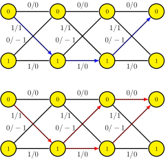
Figure 2: Illustration of joint-LP decoder outputs for the single parity-check code SPC(3,2) over DIC (starts in zero state). By ordering the trellis edges appropriately, joint-LP decoder converges to either a trellis-wise (ML) codeword $(0\,1\,0\,0;0\,0\,0\,1;.0\,0\,1\,0)$ (top dashed blue path) or a joint-decoding trellis-wise pseudo-codeword $(0\,1\,0\,0;0\,0\,.5\,.5;.5\,0\,.5\,0)$ (bottom dashed red paths). Using $\mathcal{Q}$ to project them into $\mathcal{P}(H)$, we obtain the corresponding (symbol-wise) codeword $(1,1,0)$ and joint-decoding symbolwise pseudo-codeword $(1,.5,0).$

Recently, the LP formulation has been extended to the joint decoding of a binary-input FSC and outer LDPC code [11][12]. In this case, the performance of LP decoding appears to outperform belief-propagation decoding at moderate SNR. Moreover, all integer solutions are indeed codewords and the joint decoder also has a certain ML certificate property. This allows all decoder failures to be explained by joint-decoding pseudo-codewords (see Fig. 2).

In the past, the primary value of LP decoding was as an analytical tool that allowed one to better understand iterative decoding and its modes of failure. This is because LP decoding based on standard LP solvers is quite impractical and has a superlinear complexity in the block length. This motivated several authors to propose low-complexity algorithms for LP decoding of LDPC codes in the last five years (e.g., [13, 14, 15, 16, 17, 18, 19]). Many of these have their roots in the iterative Gauss-Seidel approach proposed by Vontobel and Koetter for approximate LP decoding [14]. This approach was also studied further by Burshtein [18].

In this paper, we extend this approach to the problem of low-complexity joint LP decoding of LDPC codes and FSCs. We argue that by taking advantage of the special structure in dual-domain of the joint LP problem and replacing minima in the formulation with soft-minima, we can obtain an efficient method that solves the joint LP. While there are many ways to iteratively solve the joint LP, our main goal was to derive one as the natural analogue of TE. This should lead to an efficient method for joint LP decoding whose performance is similar to joint LP and whose complexity similar to TE. Indeed, the solution we provide is a fast, iterative, and provably convergent form of TE and update rules are tightly connected to BCJR-based TE. This demonstrates that an iterative joint LP solver with a similar computational complexity as TE is feasible (see Remark 10).

The paper is structured as follows. After briefly reviewing joint LP decoding in Sec. II, Sec. III is devoted to develop the iterative solver for the joint LP decoder, i.e., iterative joint LP decoder and its proof of convergence. Finally, we provide, in Sec. IV, the decoder performance results and conclude in Sec. V. Due to space limitations we omit many of the proofs, but they can be found in [20].

II Background: Joint LP Decoder

II-A Notation

Throughout the paper we borrow notation from [10]. Let $\mathcal{I}=\left\{1,\,\ldots,\,N\right\}$ and $\mathcal{J}=\left\{1,\,\ldots,\,M\right\}$ be sets of indices for the variable and parity-check nodes of a binary linear code. A variable node $i\in\mathcal{I}$ is connected to the set $\mathcal{N}(i)$ of neighboring parity-check nodes. Abusing notation, we also let $\mathcal{N}(j)$ be the neighboring variable nodes of a parity-check node $j\in\mathcal{J}$ when it is clear from the context. For the trellis associated with a FSC, we let $E=\left\{1,\,\ldots,\,O\right\}$ index the set of trellis edges associated with one trellis section. For each edge, $e\in E^{N}$, in the length-$N$ trellis, the functions $t(e)\rightarrow\{1,\ldots,N\}$, $s_{e}\rightarrow\mathcal{S}$, $s^{\prime}(e)\rightarrow\mathcal{S}$, $x(e)\rightarrow\{0,1\}$, and $a_{e}\rightarrow\mathcal{A}$ map this edge to its respective time index, initial state, final state, input bit, and noiseless output symbol. Finally, the set of edges in the trellis section associated with time $i$ is defined to be $\mathcal{T}_{i}=\left\{e\in E^{N}\,|\,t(e)=i\right\}$.

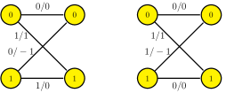
Figure 1: The dicode channel (DIC) is a binary-input FSC with a linear response of $G(z)=1-z^{-1}$ and additive Gaussian noise. If the input bits are differentially encoded prior to transmission, then the resulting channel is called the precoded dicode channel (pDIC). The state diagrams of these two channels are shown: noiseless dicode channel without (left) and with precoding (right). The edges are labeled by the input/output pair.

II-B Joint LP Decoder

Now, we describe the joint LP decoder in terms of the trellis of the FSC and the checks in the binary linear code. Let $N$ be the length of the code and $\mathbf{y}=(y_{1},y_{2},\ldots,y_{N})$ be the received sequence. The trellis consists of $(N+1)|\mathcal{S}|$ vertices (i.e., one for each state and time) and a set of at most $2N|\mathcal{S}|^{2}$ edges (i.e., one edge for each input-labeled state transition and time). The LP formulation requires one indicator variable for each edge $e\in\mathcal{T}_{i}$, and we denote that variable by $g_{i,e}$. So, $g_{i,e}$ is equal to 1 if the candidate path goes through the edge $e$ in $\mathcal{T}_{i}$. Likewise, the LP decoder requires one cost variable for each edge and we associate the branch metric $b_{i,e}$ with the edge $e$ given by

$$b_{i,e}\negthinspace\triangleq\negthinspace\begin{cases}-\ln P\negthinspace\left(y_{t(e)},s^{\prime}(e)|x(e),s(e)\right)\!\!\!&\mbox{if}\,t(e)\!>\!1\\ -\ln\left[P\left(y_{t(e)},s^{\prime}(e)|x(e),s(e)\right)\!P_{0}\left(s(e)\right)\right]\!\!\!&\mbox{if}\,t(e)\!=\!1.\end{cases}$$

Definition 1.

The trellis polytope $\mathcal{T}$ enforces the flow conservation constraints for channel decoder. The flow constraint for state $k$ at time $i$ is given by

$$\mathcal{F}_{i,k}\triangleq\left\{\mathbf{g}\in[0,1]^{N\times O}\left|\,\sum_{\begin{subarray}{c}e:s^{\prime}(e)=k\end{subarray}}g_{i,e}=\sum_{\begin{subarray}{c}e:s(e)=k\end{subarray}}g_{i+1,e}\right.\right\}.$$

Using this, the trellis polytope $\mathcal{T}$ is given by

$$\mathcal{T}\triangleq\left\{\mathbf{g}\in\bigcap_{i=1}^{N-1}\bigcap_{k\in\mathcal{S}}\mathcal{F}_{i,k}\left|\,\sum_{\begin{subarray}{c}e\in\mathcal{T}_{p}\end{subarray}}g_{p,e}=1,\,\mbox{for any}\,p\in\mathcal{I}\right.\right\}.$$

Definition 2.

Let $\mathcal{Q}$ be the projection of $\mathbf{g}$ onto the input vector $\mathbf{f}=\left(f_{1},\ldots,f_{N}\right)\in[0,1]^{N}$ defined by $\mathbf{f}=\mathcal{Q}\mathbf{g}$ with

$$f_{i}=\sum_{\begin{subarray}{c}e\in\mathcal{T}_{i}:\,x(e)=1\end{subarray}}g_{i,e}.$$

Let $\mathcal{C}\subseteq\left\{0,1\right\}^{N}$ be the length-$N$ binary linear code defined by a parity-check matrix and $\mathbf{c}=(c_{1},\ldots,c_{N})$ be a codeword. Let $\mathcal{L}$ be the set whose elements are the sets of indices involved in each parity check, or

$$\mathcal{L}=\left\{\mathcal{N}(j)\subseteq\{1,\ldots,N\}|\,j\in\mathcal{J}\right\}.$$

Then, we can define the set of codewords to be

$$\mathcal{C}=\left\{\mathbf{c}\in\left\{0,1\right\}^{N}\,\bigg{|}\,\sum_{i\in L}c_{i}\equiv 0\,\bmod 2,\,\forall\,L\in\mathcal{L}\right\}.$$

The codeword polytope is the convex hull of $\mathcal{C}$. This polytope can be quite complicated to describe though, so instead one constructs a simpler polytope using local constraints. Each parity-check $L\in\mathcal{L}$ defines a local constraint equivalent to the extreme points of a polytope in $\left[0,1\right]^{N}$.

Definition 3.

The local codeword polytope LCP($L$) associated with a parity check is the convex hull of the bit sequences that satisfy the check. It is given explicitly by

$$\mbox{LCP}(L)\triangleq\!\!\bigcap_{\begin{subarray}{c}S\subseteq L\\ \left|S\right|\text{odd}\end{subarray}}\left\{\mathbf{c}\in[0,\,1]^{N}\,\bigg{|}\sum_{i\in S}c_{i}-\!\!\!\sum_{i\in L-S}\!\!c_{i}\leq\left|S\right|\!-\!1\right\}.$$

Definition 4.

The relaxed polytope $\mathcal{P}(H)$ is the intersection of the LCPs over all checks and

$$\mathcal{P}(H) \triangleq\bigcap_{L\in\mathcal{L}}\mbox{LCP}(L).$$

Definition 5.

The trellis-wise relaxed polytope $\mathcal{P}_{\mathcal{T}}(H)$ for $\mathcal{P}(H)$ is given by

$$\mathcal{P}_{\mathcal{T}}(H)\triangleq\left\{\mathbf{g}\in\mathcal{T}\left|\mathcal{Q}\mathbf{g}\in\mathcal{P}(H)\right.\right\}.$$

Theorem 6 ([11]).

The LP joint decoder computes

$$\operatorname*{arg\,min}_{\mathbf{g}\in\mathcal{P}_{\mathcal{T}}(H)}\sum_{i\in\mathcal{I}}\sum_{\begin{subarray}{c}e\in\mathcal{T}_{i}\end{subarray}}b_{i,e}g_{i,e}$$ (1)

and outputs a joint ML edge-path if $\mathbf{g}$ is integral.

Problem-P:
$$\min_{\mathbf{g,w}}\sum_{i\in\mathcal{I}}\sum_{e\in\mathcal{T}_{i}}b_{i,e}g_{i,e}$$ subject to $$\sum_{\mathcal{B}\in\mathcal{E}_{j}}w_{j,\mathcal{B}}=1,\,\,\,\forall j\in\mathcal{J},\,\,\,\sum_{\begin{subarray}{c}e\in\mathcal{T}_{p}\end{subarray}}g_{p,e}=1,\,\mbox{for any}\,p\in\mathcal{I}$$ $$\sum_{\mathcal{B}\in\mathcal{E}_{j},\mathcal{B}\ni i}w_{j,\mathcal{B}}=\sum_{e:x(e)=1}g_{i,e},\,\,\,\forall i\in\mathcal{I},j\in\mathcal{N}\left(i\right)$$ $$\sum_{e:s^{\prime}(e)=k}g_{i,e}=\sum_{e:s(e)=k}g_{i+1,e},\,\,\,\forall i\in\mathcal{I}\setminus N,\,k\in\emph{S}$$ $$w_{j,\mathcal{B}}\geq 0,\,\,\,\forall j\in\mathcal{J},\,\mathcal{B}\in\mathcal{E}_{j},\,\,\,g_{i,e}\geq 0,\,\,\,\forall i\in\mathcal{I},\,e\in\mathcal{T}_{i}.$$

III New Results: Iterative Joint LP Decoder

III-A Iterative Joint LP Decoder Derivation

In this section, we develop an iterative solver for the joint decoding LP. There are few key steps in deriving our iterative solution for the joint LP decoding problem. For the first step, given by Problem-P, we reformulate the original LP (1) in Thm. 6 using only equality constraints involving the indicator variables $\mathbf{g}$ and $\mathbf{w}$.

The second step, given by Problem-D1, follows from standard convex analysis (e.g., see [22]). The Lagrangian dual of Problem-P is equivalent to Problem-D1 and the minimum of Problem-P is equal to the maximum of Problem-D1. From now on, we consider the Problem-D1 where the code and trellis constraints separate into two terms in the objective function. See Fig. 3 for a diagram of the variables involved.

The third step, given by Problem-D2, observes that forward/backward recursions can be used to perform the optimization over $\mathbf{n}$ and remove one of the dual variable vectors. This splitting was enabled by imposing the trellis flow normalization constraint in Problem-P only at one time instant $p\in\mathcal{I}$. This detail gives $N$ different ways to write the same LP and is an important part of obtaining update equations similar to TE.

Problem-D1:
$$\max_{\mathbf{m,n}}\sum_{j\in\emph{J}}\min_{\mathcal{B}\in\mathcal{E}_{j}}\!\left[\sum_{i\in\mathcal{B}}m_{i,j}\right]\!\!+\!\min_{e\in\mathcal{T}_{p}}\!\left[\Gamma_{p,e}\!-\!n_{p-1,s(e)}\!+\!n_{p,s^{\prime}(e)}\right]$$ subject to $$\Gamma_{i,e}\geq n_{i-1,s(e)}-n_{i,s^{\prime}(e)},\,\forall i\in\mathcal{I}\setminus p,\,e\in\mathcal{T}_{i}\vspace{-2mm}$$ and $$n_{0,k}=n_{N,k}=0,\,\forall k\in\emph{S},\vspace{-2mm}$$ where $$\Gamma_{i,e}\triangleq b_{i,e}-\delta_{x(e)=1}\sum_{j\in\mathcal{N}(i)}m_{i,j}.$$

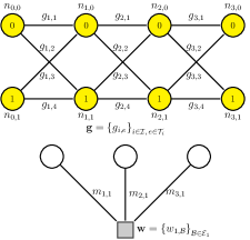
Figure 3: Illustration of primal variables $\mathbf{g}$ and $\mathbf{w}$ defined for Problem-P and dual variables $\mathbf{n}$ and $\mathbf{m}$ defined for Problem-D1 on the same example given by Fig. 2: SPC(3,2) with DIC for $N=3.$

Lemma 7.

Problem-D1 is equivalent to the Problem-D2.

Proof:

By rewriting the inequality constraint in Problem-D as

$$-n_{i,s^{\prime}(e_{i})}\leq-n_{i-1,s(e_{i})}+\Gamma_{i,e}$$

we obtain the recursive upper bound for $i=p-1$ as

$$-n_{p-1,k}$$

$$\leq\negthinspace\left.-n_{p-2,s(e_{p-1})}+\Gamma_{p-1,e}\right|_{s^{\prime}(e_{p\!-\!1})=k}$$

$$\leq\negthinspace\left.-n_{p-3,s(e_{p-2})}\negthinspace+\negthinspace\Gamma_{p-2,e}\right|_{s^{\prime}(e_{p\!-\!2})=s(e_{p\!-\!1})}\negthinspace+\negthinspace\left.\Gamma_{p-1,e}\right|_{s^{\prime}(e_{p\!-\!1})=k}$$

$$\,\,\,\,\,\,\,\,\,\,\,\,\,\,\,\,\,\,\,\,\,\,\,\,\,\,\,\,\,\,\,\,\,\,\,\,\,\,\,\,\,\,\,\,\,\,\,\,\,\,\,\,\,\,\,\,\vdots\,\,\,\,\,\,\,\,\,\,\,\,\,\,\,\,\,\,\,\,\,\,\,\,\,\,\,\,\,\,\,\,\,\,$$

$$\leq\negthinspace\left.-n_{1,s(e_{2})}\negthinspace+\negthinspace\sum_{i=2}^{p-1}\Gamma_{i,e}\right|_{s^{\prime}(e_{p\!-\!1})=k,\negthinspace s^{\prime}(e_{p\!-\!2})=s(e_{p\!-\!1}),\negthinspace\ldots,\negthinspace s^{\prime}(e_{1})=s(e_{2}).}$$

This upper bound $-n_{p-1,k}\leq-\overrightarrow{n}_{p-1,k}$ is achieved by the forward Viterbi update in Problem-D2 for $i=1,\,\ldots\,,\,p-1.$ Again, by expressing the same constraint as

$$n_{i-1,s(e_{i})}\leq\Gamma_{i,e}+n_{i,s^{\prime}(e_{i})}$$

we get recursive upper bound for $i=p+1$. Similar reasoning shows this upper bound $n_{p,k}\leq\overleftarrow{n}_{p,k}$ is achieved by the backward Viterbi update in Problem-D2 for $i=N-1,N-2,\,\ldots\,,\,p.$ See Fig. 4 for a graphical depiction of this. ∎

The fourth step, given by Problem-DS, is replacing minimum operator in Problem-D2 with the soft-minimum operation. A smooth approximation is obtained by using

$$\mbox{min}\left(x_{1},\,x_{2},\,\ldots\,,\,x_{m}\right)\approx-\frac{1}{K}\ln\sum_{i=1}^{m}\texttt{e}^{-Kx_{i}}$$

as in [14]. It is easy to verify that this log-sum-exp function converges to the minimum function as $K$ increases. Since the soft-minimum function is used in two different ways, we use different constants, $K_{1}$ and $K_{2},$ for the code and trellis terms. This Problem-DS allows one to to take derivative of (2) (giving the KKT equations, derived in Lemma 8), and represent (3) and (4) as BCJR-like forward/backward recursions (given by Lemma 9).

Problem-D2:
$$\max_{\mathbf{m}}\sum_{j\in\emph{J}}\min_{\mathcal{B}\in\mathcal{E}_{j}}\!\left[\sum_{i\in\mathcal{B}}m_{i,j}\right]\!+\min_{e\in\mathcal{T}_{p}}\!\left[\Gamma_{p,e}\!-\!\overrightarrow{n}_{p\!-\!1,s(e)}\!+\!\overleftarrow{n}_{p,s^{\prime}(e)}\right]$$ where $\overrightarrow{n}_{i,k}$ is defined for $i=1,\,\ldots\,,\,p-1$ by $$-\overrightarrow{n}_{i,k}=\min_{e\in s^{\prime-1}(k)}-\overrightarrow{n}_{i-1,s(e_{i})}+\Gamma_{i,e},\,\forall k\in\mathcal{S}\vspace{-1mm}$$ and $\overleftarrow{n}_{i,k}$ is defined for $i=N-1,N-2,\,\ldots\,,\,p$ by $$\overleftarrow{n}_{i,k}=\min_{e\in s^{-1}(k)}\overleftarrow{n}_{i+1,s^{\prime}(e_{i+1})}+\Gamma_{i+1,e},\,\forall k\in\mathcal{S}\vspace{-1.5mm}$$ starting from $$\overrightarrow{n}_{0,k}=\overleftarrow{n}_{N,k}=0,\,\forall k\in\mathcal{S}.$$

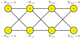
Figure 4: Illustration of Viterbi updates in Problem-D2 on the same example given by Fig. 2: DIC for $N=3$ with forward $\overrightarrow{\mathbf{n}}$ and backward $\overleftarrow{\mathbf{n}}.$

Lemma 8.

The unique maximum of (2) over $\left\{m_{p,j^{\prime}}\right\}_{j^{\prime}\in\mathcal{N}(p)}$ can be found using the KKT equations, and an iterative solution for $p\in\mathcal{I}$ is given by

$$m_{p,j^{\prime}}=M_{p,j^{\prime}}+\frac{\gamma_{p}}{K_{1}},\,\,\,M_{p,j^{\prime}}\triangleq\frac{1}{K_{1}}\,\ln\,\frac{1-l_{p,j^{\prime}}}{1+l_{p,j^{\prime}}}$$

for $j^{\prime}\in\mathcal{N}(p)$ where

$$l_{p,j^{\prime}}\triangleq\prod_{i\in\mathcal{N}(j^{\prime})\setminus p}\tanh\left(\frac{K_{1}m_{i,j^{\prime}}}{2}\right),$$

$$\gamma_{p}\triangleq\ln\,\frac{\sum_{e\in\mathcal{T}_{p}:x(e)=0}\texttt{e}^{-K_{2}\left(\Gamma_{p}-\overrightarrow{n}_{p-1,s(e)}+\overleftarrow{n}_{p,s^{\prime}(e)}\right)}}{\sum_{e\in\mathcal{T}_{p}:x(e)=1}\texttt{e}^{-K_{2}\left(\Gamma_{p}-\overrightarrow{n}_{p-1,s(e)}+\overleftarrow{n}_{p,s^{\prime}(e)}\right)}}.$$

Problem-DS:
$\displaystyle\max_{\mathbf{m}}\,\,-\frac{1}{K_{1}}\sum_{j\in\emph{J}}\ln\sum_{\mathcal{B}\in\mathcal{E}_{j}}\texttt{e}^{-K_{1}\left\{\sum_{i\in\mathcal{N}(j)}m_{i,j}\mathbbm{1}_{\mathcal{B}}(i)\right\}}$ (2) $\displaystyle-\frac{1}{K_{2}}\ln\sum_{e\in\mathcal{T}_{p}}\texttt{e}^{-K_{2}\left\{\Gamma_{p,e}-\overrightarrow{n}_{p-1,s(e)}+\overleftarrow{n}_{p,s^{\prime}(e)}\right\}}$ where $\mathbbm{1}_{\mathcal{B}}\left(i\right)$ is the indicator function of the set $\mathcal{B},$ $\overrightarrow{n}_{i,k}$ is defined for $i=1,\,\ldots\,,\,p-1$ by $$-\overrightarrow{n}_{i,k}=-\frac{1}{K_{2}}\ln\!\!\sum_{e_{i}\in s^{\prime-1}(k)}\!\!\texttt{e}^{-K_{2}\left\{-\overrightarrow{n}_{i-1,s(e_{i})}+\Gamma_{i,e}\right\}},$$ (3) and $\overleftarrow{n}_{i,k}$ is defined for $i=N-1,N-2,\,\ldots\,,\,p$ by $\displaystyle\overleftarrow{n}_{i,k}$ $\displaystyle=-\frac{1}{K_{2}}\ln\!\!\!\sum_{e_{i+1}\in s^{-1}(k)}\!\!\!\texttt{e}^{-K_{2}\left\{\overleftarrow{n}_{i+1,s^{\prime}(e_{i+1})}+\Gamma_{i+1,e}\right\}}$ (4) starting from $$\overrightarrow{n}_{0,k}=\overleftarrow{n}_{N,k}=0,\,\forall k\in\mathcal{S}.$$

Lemma 9.

Equations (3) and (4) are equivalent to the BCJR-based forward and backward recursion given by (5), (6), and (7).

Now, we have all the pieces to complete the algorithm. As the last step, we combine the results of Lemma 8 and 9 to obtain the iterative solver for the joint decoding LP, which is summarized in Algorithm 1.

Remark 10.

While resulting Algorithm 1 has the bit-node update different from standard belief propagation (BP), we note that setting $K_{1}=1$ in the inner loop gives the exact BP check-node update and setting $K_{2}=1$ in the outer loop gives the exact BCJR channel update. In fact, one surprising result of this work is that such a small change to the BCJR-based TE update provides an iterative solver for the LP whose complexity similar to TE. It is also possible to prove the convergence of a slightly modified iterative solver that is based on a less efficient update schedule.

Algorithm 1 Iterative Joint Linear-Programming Decoding

• Step 1. Initialize $m_{i,j}=0$ for $i\in\mathcal{I},\,j\in\mathcal{N}\left(i\right)$ and iteration count $\ell=0.$

• Step 2. Update Outer Loop: For $i\in\mathcal{I}$,

  • (i) Compute bit-to-trellis message

    $$\lambda_{i,e}=\texttt{e}^{-K_{{}_{2}}\Gamma_{i,e}}\vspace{-2mm}$$

    where

    $$\Gamma_{i,e}=b_{i,e}-\delta_{x(e)=1}\sum_{j\in\mathcal{N}(i)}m_{i,j}.\vspace{-1mm}$$

  • (ii) Compute forward/backward trellis messages

    $$\!\!\!\!\!\!\!\!\!\!\!\!\!\!\!\!\!\!\alpha_{i+1}\left(k\right)\!=\!\frac{\sum_{e\in s^{\prime-1}(k)}\alpha_{i}\left(s(e)\right)\cdot\lambda_{i+1,e}}{\sum_{k}\sum_{e\in s^{\prime-1}(k)}\alpha_{i}\left(s(e)\right)\cdot\lambda_{i+1,e}}$$ (5)

    $$\!\beta_{i-1}\left(k\right)\!=\!\frac{\sum_{e\in s^{-1}(k)}\beta_{i}\left(s^{\prime}(e)\right)\cdot\lambda_{i,e}}{\sum_{k}\sum_{e\in s^{-1}(k)}\beta_{i}\left(s^{\prime}(e)\right)\cdot\lambda_{i,e}},$$ (6)

    where $\beta_{N}\left(k\right)=\alpha_{0}\left(k\right)=1/\left|\mathcal{S}\right|$ for all $k\in\mathcal{S}$.

  • (iii) Compute trellis-to-bit message $\gamma_{i}$

    $$\!\!\!\!\!\!\!\!\gamma_{i}\!=\!\mbox{log}\,\frac{\sum_{e\in\mathcal{T}_{i}:x(e)=0}\alpha_{i-1}\left(s(e)\right)\lambda_{i,e}\beta_{i}\left(s^{\prime}(e)\right)}{\sum_{e\in\mathcal{T}_{i}:x(e)=1}\alpha_{i-1}\left(s(e)\right)\lambda_{i,e}\beta_{i}\left(s^{\prime}(e)\right)}$$ (7)

• Step 3. Update Inner Loop for $\ell_{\mbox{inner}}$ rounds: For $i\in\mathcal{I}$,

  • (i) Compute bit-to-check msg $m_{i,j}$ for $j\in\mathcal{N}\left(i\right)$

    $$m_{i,j}=M_{i,j}+\frac{\gamma_{i}}{K_{1}}$$

  • (ii) Compute check-to-bit msg $M_{i,j}$ for $j\in\mathcal{N}\left(i\right)$

    $$M_{i,j}=\frac{1}{K_{1}}\,\ln\,\frac{1-l_{i,j}}{1+l_{i,j}}$$

    where

    $$l_{i,j}=\prod_{r\in\mathcal{N}\left(j\right)\setminus i}\tanh\left(\frac{K_{1}m_{r,j}}{2}\right)$$

• Step 4. Compute hard decisions and stopping rule

  • (i) For $i\in\mathcal{I}$,

    $$\hat{f}_{i} =\begin{cases}1&\mbox{if}\,\,\,\gamma_{i}<0\\ 0,&\mbox{otherwise}\end{cases}$$

  • (ii) If $\mathbf{\hat{f}}$ satisfies all parity checks or the iteration number, $\ell_{\mbox{outer}}$, is reached, stop and output $\mathbf{\hat{f}}$. Otherwise increase $\ell$ by 1 and go to Step 2.

III-B Convergence Analysis

This section considers the convergence properties of the proposed Algorithm 1. Although we have always observed convergence of Algorithm 1 in simulation, our proof requires a modified update schedule that is less computationally efficient. Following Vontobel’s approach in [14], which is based on general properties of Gauss-Seidel-type algorithms for convex minimization, we show that the modified version Algorithm 1 is guaranteed to converge. Moreover, a feasible primal solution can be obtained that is arbitrarily close to the solution of Problem-P.

The modified update rule for Algorithm 1 consists of cyclically, for each $p=1,\ldots,N$, computing the quantity $\gamma_{p}$ (via step 2 of Algorithm 1) and then updating $m_{p,j}$ for all $j\in\mathcal{N}(p)$ (based on step 3 of Algorithm 1). The drawback of this approach is that one BCJR update is required for each bit update, rather than for $N$ bit updates. This modification allows us to interpret Algorithm 1 as a Gauss-Seidel-type algorithm. Therefore, the next theorem can be seen as a natural generalization of [14][18].

Problem-PS:
$$\min_{\mathbf{g,w}}\sum_{i\in\mathcal{I}}\sum_{e\in\mathcal{T}_{i}}b_{i,e}g_{i,e}-\frac{1}{K_{1}}\sum_{j\in\mathcal{J}}H(w_{j})-\frac{1}{K_{2}}H(g_{p})$$ subject to the same constraints as Problem-P.

Theorem 11.

Let $P^{*}$ and $\tilde{P}$ be the minimum value of Problem-P and Problem-PS and denote $\tilde{\mathbf{g}}$ be the optimum solution of Problem-PS. For any $\delta>0$, there exist sufficiently large $K_{1}$ and $K_{2}$ such that sufficient many iterations of the modified Algorithm 1 yields $\mathbf{\tilde{g}}$ which is feasible in Problem-P and satisfies

$$0\leq\frac{\tilde{P}-P^{*}}{N}\leq\delta.$$

IV Performance of Iterative Joint LP Decoder

To validate proposed solutions for the problem of the joint decoding of a binary-input FSC and outer LDPC, we use the following two simulation setups:

• For preliminary studies, we use $(3,\,5)$-regular binary LDPC codes with length 455 on the precoded dicode channel (pDIC)

• For practical study, we use a $(3,\,27)$-regular binary LDPC code with length 4923 and rate 8/9 on the class-II Partial Response (PR2) channel used as a partial-response target for perpendicular magnetic recording.

All parity-check matrices were chosen randomly except that double-edges and four-cycles were avoided. Since the performance depends on the transmitted codeword, the results were obtained for a few chosen codewords of fixed weight. The weight was chosen to be roughly half the block length, giving weights 226 and 2462.

Fig. 5 shows the decoding results based on the Algorithm 1 compared with the joint LP decoding performed in the dual domain using MATLAB in the first setup. The choice of parameters and scheduling scheme has yet to be optimized. Instead, we use a simple scheduling update scheme: variables are updated cyclically with 5 inner loop iterations after single outer iteration with $K_{1}=1000\,\mbox{and}\,K_{2}=100$. Somewhat interestingly, we find that iterative joint LP decoding WER curve loses about 0.2 dB at low SNR. This may be caused by using too few iterations or finite values of $K_{1}$ and $K_{2}$. But, at high SNR this gap disappears and the curve converges towards the error rate predicted for joint LP decoding. This shows that joint LP decoding outperforms belief-propagation decoding for short length code at moderate SNR with the predictability of LP decoding. Of course this can be achieved with a computational complexity similar to turbo equalization.

Fig. 6 shows the decoding results based on the Algorithm 1 compared with the state-based JIMPD algorithm described in [23] in more practical scenario. To make a fair comparison, we fix the maximum iteration count, $\ell_{\mbox{outer}}\left(\ell_{\mbox{inner}}+1\right)$ of each algorithm to roughly 1000 and choose $K_{1}=1000\,\mbox{and}\,K_{2}=10$ for Algorithm 1. Surprisingly, we find that iterative joint LP decoding WER curve with Algorithm 1 wins over JIMPD at all SNR with substantial gains. Also, the slope difference between two curves anticipate greatly better error-floor performance of Algorithm 1. This shows that joint LP decoding outperforms belief-propagation decoding even for long length code at all SNR with a computational complexity similar to TE.

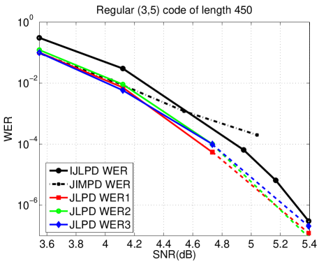
?figurename? 5: This figure shows comparison between the joint LP decoding (JLPD), joint iterative message-passing decoding (JIMPD), and iterative joint LP decoding (IJLPD) on the pDIC with AWGN for random (3,5) regular LDPC codes of length $N=450$. The curves shown are the JLPD WER (solid), JLPD WER prediction (dashed), JIMPD WER (dash-dot), and IJLPD WER (circle-solid). The dashed curves are computed using the union bound based on joint-decoding pseudo-codewords observed at 2.67 dB as described in [11] and the dash-dot curves are obtained using the state-based JIMPD described in [23]. The circle-solid curves are computed using Algorithm 1. Note that SNR is defined as channel output power divided by $\sigma^{2}$.

V Conclusions

In this paper, we consider the problem of low-complexity joint linear-programming (LP) decoding of low-density parity-check codes and finite-state channels. We present a novel iterative solver for the joint LP decoding problem. This greatly reduces the computational complexity of the joint LP solver by exploiting the LP dual problem structure. Its main advantage is that it provides the predictability of LP decoding and significant gains over turbo equalization (TE) with a computational complexity similar to TE.

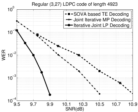
Figure 6: This figure shows comparison between the iterative joint LP decoding and other TE based methods on the PR2 channel with AWGN for random (3,27) regular LDPC codes of length $N=4923$. The curves shown are the joint iterative LP decoding WER (solid), the stated-based joint iterative message-passing (MP) decoding WER (dash-dot) described in [23], and the soft output Viterbi algorithm (SOVA)-based TE decoding WER (dashed) taken from [24]. Note that SNR is defined as channel output power divided by $\sigma^{2}$.

- [1] C. Douillard, M. Jézéquel, C. Berrou, A. Picart, P. Didier, and A. Glavieux, “Iterative correction of intersymbol interference: Turbo equalization,” Eur. Trans. Telecom., vol. 6, no. 5, pp. 507–511, Sept. – Oct. 1995.
- [2] R. G. Gallager, “Low-density parity-check codes,” Ph.D. dissertation, M.I.T., Cambridge, MA, USA, 1960.
- [3] R. R. Müller and W. H. Gerstacker, “On the capacity loss due to separation of detection and decoding,” IEEE Trans. Inform. Theory, vol. 50, no. 8, pp. 1769–1778, Aug. 2004.
- [4] W. E. Ryan, “Performance of high rate turbo codes on a PR4-equalized magnetic recording channel,” in Proc. IEEE Int. Conf. Commun. Atlanta, GA, USA: IEEE, June 1998, pp. 947–951.
- [5] L. L. McPheters, S. W. McLaughlin, and E. C. Hirsch, “Turbo codes for PR4 and EPR4 magnetic recording,” in Proc. Asilomar Conf. on Signals, Systems & Computers, Pacific Grove, CA, USA, Nov. 1998.
- [6] M. Öberg and P. H. Siegel, “Performance analysis of turbo-equalized dicode partial-response channel,” in Proc. 36th Annual Allerton Conf. on Commun., Control, and Comp., Monticello, IL, USA, Sept. 1998, pp. 230–239.
- [7] M. Tüchler, R. Koetter, and A. Singer, “Turbo equalization: principles and new results,” IEEE Trans. Commun., vol. 50, no. 5, pp. 754–767, May 2002.
- [8] B. M. Kurkoski, P. H. Siegel, and J. K. Wolf, “Joint message-passing decoding of LDPC codes and partial-response channels,” IEEE Trans. Inform. Theory, vol. 48, no. 6, pp. 1410–1422, June 2002.
- [9] J. Feldman, “Decoding error-correcting codes via linear programming,” Ph.D. dissertation, M.I.T., Cambridge, MA, 2003.
- [10] J. Feldman, M. J. Wainwright, and D. R. Karger, “Using linear programming to decode binary linear codes,” IEEE Trans. Inform. Theory, vol. 51, no. 3, pp. 954–972, March 2005.
- [11] B.-H. Kim and H. D. Pfister, “On the joint decoding of LDPC codes and finite-state channels via linear programming,” in Proc. IEEE Int. Symp. Information Theory, Austin, TX, June 2010, pp. 754–758.
- [12] M. F. Flanagan, “A unified framework for linear-programming based communication receivers,” Feb. 2009, [Online]. Available: http://arxiv.org/abs/0902.0892.
- [13] T. Wadayama, “Interior point decoding for linear vector channels based on convex optimization,” IEEE Trans. Inform. Theory, vol. 56, no. 10, pp. 4905–4921, Oct. 2010.
- [14] P. Vontobel and R. Koetter, “Towards low-complexity linear-programming decoding,” in Proc. Int. Symp. on Turbo Codes & Related Topics, Munich, Germany, April 2006.
- [15] P. Vontobel, “Interior-point algorithms for linear-programming decoding,” in Proc. 3rd Annual Workshop on Inform. Theory and its Appl., San Diego, CA, Feb. 2008.
- [16] M. Taghavi and P. Siegel, “Adaptive methods for linear programming decoding,” IEEE Trans. Inform. Theory, vol. 54, no. 12, pp. 5396–5410, Dec. 2008.
- [17] T. Wadayama, “An LP decoding algorithm based on primal path-following interior point method,” in Proc. IEEE Int. Symp. Information Theory, Seoul, Korea, June 2009, pp. 389–393.
- [18] D. Burshtein, “Iterative approximate linear programming decoding of LDPC codes with linear complexity,” IEEE Trans. Inform. Theory, vol. 55, no. 11, pp. 4835–4859, Oct. 2009.
- [19] M. Punekar and M. F. Flanagan, “Low complexity linear programming decoding of nonbinary linear codes,” in Proc. 48th Annual Allerton Conf. on Commun., Control, and Comp., Monticello, IL, Sept. 2010.
- [20] B.-H. Kim and H. D. Pfister, “Joint decoding of LDPC codes and finite-state channels via linear-programming,” Jan. 2011, submitted to IEEE J. Select. Topics in Signal Processing. [Online]. Available: http://arxiv.org/abs/1102.1480.
- [21] M. F. Flanagan, V. Skachek, E. Byrne, and M. Greferath, “Linear-programming decoding of nonbinary linear codes,” IEEE Trans. Inform. Theory, vol. 55, no. 9, pp. 4134–4154, Sept. 2009.
- [22] S. Boyd and L. Vandenberghe, Convex Optimization. Cambridge University Press, 2004.
- [23] A. Kavčić, X. Ma, and M. Mitzenmacher, “Binary intersymbol interference channels: Gallager codes, density evolution and code performance bounds,” IEEE Trans. Inform. Theory, vol. 49, no. 7, pp. 1636–1652, July 2003.
- [24] S. Jeon, X. Hu, L. Sun, and B. Kumar, “Performance evaluation of partial response targets for perpendicular recording using field programmable gate arrays,” IEEE Trans. Magn., vol. 43, no. 6, pp. 2259–2261, 2007.