Troubles of describing multiple pion production in chiral
dynamics.
N. N. Achasova111e-mail: achasov@math.nsc.ru, A. A. Kozhevnikova,b222e-mail: kozhev@math.nsc.ru aLaboratory of Theoretical Physics, S. L. Sobolev Institute for Mathematics 630090, Novosibirsk, Russian Federation bNovosibirsk State University 630090, Novosibirsk, Russian Federation
Abstract
Generalized Hidden Local Symmetry (GHLS) model as the chiral model
of pseudoscalar, vector, and axial vector mesons and their
interactions containing also the couplings of strongly interacting
particles with electroweak gauge bosons, is confronted with the
ALEPH data on the decay and
BABAR and CMD data on the reaction
. It is shown that both the
invariant mass spectrum of final pions in decay calculated
in the GHLS framework with the single resonance and
the cross section calculated in
the above framework with the single resonance,
disagree with the experimental data. The modifications of GHLS
model based on inclusion of two additional heavier axial vector
mesons , in the decay and
the vector mesons , in
are shown to be necessary for the
good description of the above data.
1. Introduction. The theory aimed at describing low energy
hadron processes should be formulated in terms of effective
colorless degrees of freedom introduced on the basis of
spontaneously broken approximate chiral symmetry . This is the symmetry of QCD Lagrangian
(1)
relative independent rotations of right and left fields of
approximately massless quarks:
(2)
where . The pattern of the spontaneous
breaking is .
According to the Goldstone theorem, spontaneous breaking of global
symmetry results in appearance of massless fields. In our case
they are light mesons , , , ,
, , , . The transformation law
where
, and
(6)
fixes the Lagrangian of interacting Goldstone mesons:
Dots mean the terms with
higher derivatives. Upon adding the term which explicitly breaks chiral
symmetry, Goldstone bosons become massive.
Pseudoscalar mesons are produced via intermediate vector and
axial resonances, hence one should include vector and axial
vector mesons in a chiral invariant way. There are a number of
chiral models of pseudoscalar, vector, and axial mesons and their
interaction [1]. The problem of testing chiral
models of the vector meson interactions with Goldstone bosons is
acute. The present report is devoted to reviewing the attempts to
confront one of the chiral models, the Generalized Hidden Local
Symmetry (GHLS) model [2, 3, 4], with the
data on the decay
[5] in the axial vector channel, and the data on the
reaction [6, 7] in the
vector channel, both in the state with the isospin one.
2. Generalized Hidden Local Symmetry Model Lagrangian. The
Generalized Hidden Local Symmetry (GHLS) model
[2, 3, 4] as the chiral model based on
nonlinear realization of chiral symmetry, is of a special
interest because some interesting two- and three-particle decays,
for example, and ,
were analyzed in its framework [4]. ”Hidden” means
that if then the transformation law
implies one where transforms vector meson fields in a
gauge-like manner as . ”Generalized hidden” means that axial vector mesons are
included. One of the virtues of GHLS model is that the sector of
electroweak interactions is introduced in such a way that the low
energy relations in the sector of strong interactions are not
violated upon inclusion of photons and electroweak gauge bosons.
The GHLS lagrangian includes pseudoscalar, vector, and axial
vector fields , , and , respectively. In the
gauge , and after rotating away
the axial vector- mixing by choosing
(7)
where is meson field, is the coupling constant
to be related to , and
(8)
the relevant terms corresponding to strong interactions look like
(9)
The lagrangian contains a number of free parameters
. The terms with free
parameters are necessary for cancelation of
momentum dependence in the vertex. They are chosen in
accord with Refs. [3, 4] in such a way that among
the terms with higher derivatives those with
are set to zero, and only the
terms are included, with the additional
assumption about the arbitrary constants
multiplying the lagrangian terms. The remaining ones
and should be related like
(10)
in order to provide the desired cancelation. The notations,
assuming the restriction to the sector of the non-strange mesons,
are
(11)
where , are the vector meson and
pseudoscalar pion fields, respectively, is the axial
vector field [not meson, see Eq. (7)],
is the isospin Pauli matrices. Free parameters
, and of the GHLS lagrangian with
index are bare parameters before renormalization (see below);
stands for commutator. Hereafter the boldface characters,
cross (), and dot () stand for vectors, vector
product, and scalar product, respectively, in the isotopic space.
GHLS lagrangian includes also electroweak sector. In what follows
we will neglect the terms quadratic in electroweak coupling
constants keeping only the terms linear in above couplings. These
terms describe the interaction of , , and mesons
with electroweak gauge bosons and look as [3, 4]
(12)
Upon neglecting the weak neutral current contribution, the
charged weak and electromagnetic sectors are taken into account
via [3, 4],
(13)
are the fields of
bosons, is the electroweak gauge coupling constant.
In the subgroup of the flavor group of strong
interactions one has
, is the element of
Cabibbo-Kobayashi-Maskawa matrix, stands for the
field of the photon, is the elementary charge, and
is the charge matrix restricted to the sector of
nonstrange mesons. In the spirit of chiral perturbation theory, as
the first step in obtaining necessary terms, one should expand the
matrix into the series over . The
second step is the renormalization necessary for canonical
normalization of the pion kinetic term. The renormalization is
[3, 4]
(14)
where Close
examination of Eq. (12) shows that the expansion includes
the point-like interaction
Analogous term
appears when one restores electromagnetic field. Since there are
no experimental indications on point-like
vertex, we set
(15)
This
relation removes also the above point-like
vertex.
3. The amplitude of the transition . Expanding the GHLS lagrangian into the
series in the ratio of the pion momentum to the pion decay
constant MeV, first, one obtains the relations
(16)
We fix
hereafter from the experimental value of the
decay width leaving as free parameter.
Second, the lagrangian describing the decay is found
to be
(17)
The amplitude of the decay
calculated from
Eq. (17) can be written as follows:
,
(18)
where is the
polarization four-vector of meson, and
, where
Hereafter interchanges pion momenta and
, stands for the Lorentz scalar product of
four-vectors, and . Parameters and
are the combinations of the GHLS parameters:
(19)
Notice that
the amplitude (18) respects the Adler condition: it
vanishes in the chiral limit when the four-momentum
of any final pion vanishes. Such a property is the manifestation
of the chiral invariance.
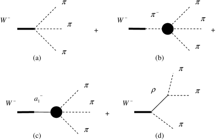
The amplitude of the decay
incorporates the transition . In GHLS, the
latter is given by the diagrams shown in Fig. 1.
Figure 1: Diagrams schematically describing the
transition . Shaded circles depict the
transition including both the point-like and -exchange
contributions. Permutations of pion momenta are understood.
Necessary terms are obtained from the low momentum expansion of
electroweak piece of GHLS lagrangian Eq. (12) and look like
(20)
where the vector denotes transverse
charged components of the isotopic vector. The amplitude of the
decay corresponding to
the diagrams Fig. 1 is
, where
is the polarization four-vector of
boson and the axial decay current looks like
(21)
In the above expressions, , , and are the
inverse propagators of , , and mesons,
respectively. The terms corresponding to the diagrams (a), (b),
(c), and (d) in Fig. 1 are easily identified by these
propagators.
The spectrum of the three pion state in the decay
normalized to its branching
fraction is
(22)
, is the Fermi constant, and is the
width of lepton. The transverse and longitudinal spectral
functions are, respectively,
(23)
where is the element of Lorentz-invariant phase
space volume of the system . The numerical
integration shows that is by about three orders of
magnitude smaller than in all allowed kinematical range
and hence can be neglected.
4. Results for . The
”canonical” choice of free GHLS parameters [4]
(24)
and
, results in the spectrum which
disagrees with the data both in lower branching ratio
and in the shape
of the spectrum. Upon the variation of free parameters of the
single resonance contribution listed in Eq. (24)
one obtains the can reproduce the branching ratio
but the shape of
the spectrum is not reproduced. Inclusion of additional higher
derivative terms [8] to the suggested in
Refs. [3, 4] and subjected to the fitting in the
present work minimal set Eq. (24) cannot improve the
situation. Indeed, even the minimal set Eq. (24) results
in a rather fast growth of the decay width with the
energy increase. Additional higher derivative terms would make
the growth to be explosive. Restricting such a growth would
require phenomenological form factors with free parameters. We
believe that the dynamical explanation of the shape of the
spectrum based on additional axial vector resonances
, would be preferable. Note that
there are indications on such resonances, both theoretical
[9, 10] and experimental [11, 12, 13].
Taking , into account reduces to adding
two diagrams similar to one in Fig. 1(c), with the
replacement of by and
. Since there is no available information
concerning their couplings, the above resonances are included in
a way analogous to . This prescription results in the
amplitudes of the decays
vanishing when the four-momentum of any final pion vanishes. That
is, the way of inclusion additional resonances respects chiral
symmetry. The total set of the fitted parameters is first taken to
be
The parameters , , characterize
the decay amplitude similar to
Eq. (18), (Troubles of describing multiple pion production in chiral
dynamics.) in the case of ,
while parameterizes the coupling
as . Compare with
Eq. (18). Analogously for . The fit
chooses and turns out to be insensitive to this
parameter leaving . The quality of
the fit can be considerably improved upon fixing but
adding new parameter -the phase of the
contribution. Such phase imitates possible mixing among ,
, resonances. The results of such
type of the fit are given in the column variant A of the Table
1.
Table 1: The values of free parameters of GHLS
model obtained from the unconstrained fit of the ALEPH data on
the decay [5]
(variant A), and the fit with the constrain preserving
universality (variant B). Also shown are the corresponding
calculated original [3, 4] GHLS parameters and
the magnitudes of branching fractions of the above decay.
Figure 2: The spectrum of in
decay in the variant A of the Table 1. The
dashed line corresponds to the sum of the diagrams
Fig. 1. See the text for more detail.
Using Eq. (16), (19), and obtaining
from [11] one
can compare the fitted GHLS parameters with the ”canonical” ones
Eq. (24). To this end one should use Eq. (15)
and (16) to obtain
(25)
These GHLS
parameters are marked in the Table 1 as
”calculated”. Since the basis of inclusion of heavier resonances
and here is purely
phenomenological, specifically, there is no analog of gauge
coupling constant , we do not recalculate
and
similar to Eq. (25). One can see that the obtained
is in disagreement with the universality
condition , which demands , see
Eq. (16). Hence we fulfill also the partially
constrained fit with , in order to preserve universality
of the couplings. The results are presented as the variant
B in the Table 1. The total spectrum in this
variant is not shown because it looks the same as in
Fig. 2. Note that in the variant A the visible
peak position is lower than that of
despite of the fact that their bare masses are in
opposite relation, see the Table 1. This can be
explained as follows. The dominant decay mode of ,
resonances is the one. Its partial
width grows rapidly with energy increase reaching the figures
compatible with bare mass itself. The combined action of the
strong energy dependence of the partial width and its large
magnitude shifts the visible peak towards the lower energies
[14]. The evaluation shows that the width of
and its growth are stronger as compared to
. Hence the visible position of the former appears at
lower energy than the visible position of .
Of a special interest is the width of the radiative decay
. This decay originates from both the
transition followed by the transition
and by the direct transition.
The necessary amplitudes can be read off Eq. (20). The
resulting decay width is
(26)
where is the fine structure constant. Notice, that the
above expression for is written
with the counter terms taken into account. The
decay amplitude without counter terms is
proportional to the combination which
vanishes at any choice of GHLS parameters because of the relations
(16) and (19). The evaluation of
with the parameters from the
variants A and B of the Table 1 gives the figures
of the order of few MeV due to large values of in the
Table 1 chosen by the fits. This is in disagreement
with the measured
keV [15]. Hence, one should further constrain the fit in
order to incorporate the above radiative width upon expressing
parameter from Eq. (26). When fitting,
the central value of the radiative width. To provide
the universality of the couplings, is kept fixed,
too. It is found out that the fit with the fixed parameters
and gives rather poor description with . The peculiar feature of the fit is that it
chooses , the phase of the
contribution, but is almost insensitive to the rather
wide variations around above central value. Hence, we fix
, but introduce a new free parameter
whose meaning is , where
effectively takes into account the
contributions to the resonance width other than
one, for example,
, . They may be effective
for the off-mass-shell meson. The results of such type of
the fit are presented as the variant C in the Table
2.
Table 2: The values of free parameters of GHLS
model obtained from the fit of the ALEPH data on the decay
[5] constrained in a
way as to fix and .
Variant C is the fit including
contributions. Variant D
includes only ones. Also shown are the
corresponding calculated original [3, 4] GHLS
parameters and the magnitudes of branching fractions of the
above decay.
parameter
variant C
variant D
[GeV]
(calculated)
(calculated)
(calculated)
(calculated)
(calculated)
(calculated)
[GeV2]
[GeV]
[GeV]
45/102
95/107
The spectrum of the system evaluated with the
parameters of variant C is shown with the solid line in
Fig. 3. Note that the found
GeV2 corresponds to
the portion of the decay channels different from
one, at the level
. This estimate
can be obtained from the calculated
. The above estimate
demonstrates that the additional contribution to the width
beside the GHLS one is very small. Since the contribution of the
resonance is rather small, see
Fig. 3, we fulfill the fit in which the
contribution of the resonance is absent. The parameters found in
such type of the fit are listed as the variant D in the Table
2.
Figure 3: The same as in Fig. 2,
but for the parameters of the variant C of the Table
2.
5. GHLS and the reaction at
1 GeV. Because the evaluation of the four pion
decay width of the -like resonances is very time-consuming,
we study the predictions of GHLS model for the reaction
with the ”canonical” choice of
free parameters (24). The set of the diagrams necessary
for calculation of the amplitude is shown in Fig. 4,
5, and 6.
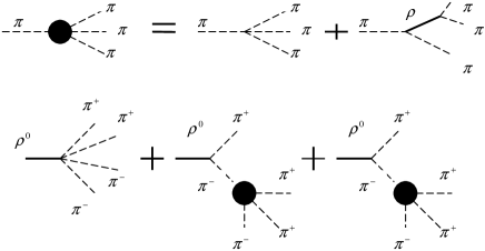
Figure 4: The diagrams due to
HLS lagrangian. Shaded circles in the diagrams stand
for the transition shown in the first line of this
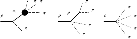
figure.Figure 5: The diagrams due to
and couplings (GHLS). The shaded
circle stands for the total amplitude similar to
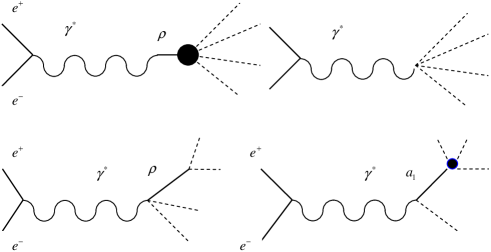
Eq. (18).Figure 6: Diagrams describing process .
Shaded circle in the first diagram stands for the sum of the
diagrams in Fig. 4 and 5. The last three diagrams are
due to the point-like , , and couplings from the
lagrangian (20).
This set includes the resonance production , where
(see below), and the
point-like transitions due to the GHLS electromagnetic coupling
(20) where free GHLS parameters are chosen in accord
with (24).
The results of evaluation of the cross section of the reaction
in the GHLS model with the
”canonical choice” (24) are shown in Fig. 7
and 8 with the dotted line.
Figure 7: Fitting CMD-2 data [6].Figure 8: Fitting BaBaR data [7].
One can see that the simplest variant with the single
s-channel resonance cannot reproduce the data at
GeV. Upon including the ,
resonances with the couplings chosen by
analogy with the ones one can improve the description
of the data [6, 7]. The results of fitting CMD-2 data
[6] and the BABAR ones [7] in the fixed width
approximation for the ,
resonances with the PDG masses and widths [11] are shown in
Fig. 7 and 8. It appears that at
GeV the joint contribution of the
, resonances is by the factor
of thirty grater than the contribution of .
6. Conclusion. The heavier axial vector resonances
and contributions should be
added to the one in order to obtain the correct shape
of the spectrum in the decay . Similar
problem is found in the vector channel
. The contributions of heavier
resonances and are required
for correct description of experimental data at energy
GeV. However, contrary to the case of the
vector channel where additional contributions of and
at the above energy exceed the
one, in the axial vector channel , each of
the additional contributions is smaller in magnitude than the
contribution of pure GHLS with the single fitted resonance.
See Fig. 2 and 3. But they
contribute almost coherently resulting in the acceptable shape of
the spectrum and the acceptable magnitude of the branching
fraction .
References
[1]
Ulf-G. Meissner, Phys.Rept. 161, 213 (1988).
[2]
M. Bando, T. Kugo, S. Uehara et al., Phys.Rev.Lett. 54,
1215 (1985).
[3]
M. Bando, T. Fujiwara, and K. Yamawaki, Progr.Theor.Phys. 79,
1140 (1988).
[4]
M. Bando, T. Kugo, and K. Yamawaki, Phys.Rept. 164, 217
(1988). See also review [1].
[5]
S. Schael et al. (ALEPH Collaboration), Phys.Rept.421,
191 (2005).
[6]
R. R. Akhmetshin, et al. (CMD-2 Collab.), Phys.Lett.
B475, 190 (2000) [arXiv:hep-ex/9912020v1].
[7]
B. Aubert, et al. (BaBaR Collab.), Phys.Rev. D71,
052001 (2005) [arXiv:hep-ex/0502025v1].
[8]
Bing An Li and Yue-Liang Wu, Mod.Phys.Lett.A22, 683(2007)
[arXiv:hep-ph/0509054].
[9]
R. Kokoski and N. Isgur, Phys.Rev.D35, 907 (1987).
[10]
S. Godfrey and N. Isgur, Phys.Rev.D32, 189 (1985).
[11]
C. Amsler, et al., Phys.Lett.B667, 1 (2008).
[12]
D. V. Amelin, et al., (the VES Collaboration), Phys. Lett.
B356, 595 (1995).
[13]
D. Asner, et al. (CLEO Collaboration), Phys.Rev.D61,
012002(2000) [arXiv:hep-ex/9902022v1].
[14]
N. N. Achasov and A. A. Kozhevnikov,
Phys.Rev.D62,117503(2000) [arXiv:hep-ph/0007205v2];
Yad.Fiz.65,158(2002) [Phys.Atom.Nucl.65153(2002)].
[15]
M. Zielinski et al., Phys.Rev.Lett. 52, 1195 (1984).