Band theory of spatial dispersion in magnetoelectrics

Abstract

Working in the crystal-momentum representation, we calculate the optical conductivity of noncentrosymmetric insulating crystals at first order in the wave vector of light. The time-even part of this tensor describes natural optical activity and the time-odd part describes nonreciprocal effects such as gyrotropic birefringence. The time-odd part can be uniquely decomposed into magnetoelectriclike and purely quadrupolar contributions. The magnetoelectriclike component reduces in the static limit to the traceless part of the frozen-ion static magnetoelectric polarizability while at finite frequencies it acquires some quadrupolar character in order to remain translationally invariant. The expression for the orbital contribution to the conductivity at transparent frequencies is validated by comparing numerical tight-binding calculations for finite and periodic samples.

I Introduction

Electric and magnetic effects are closely coupled in magnetoelectric (ME) materials. These are insulators with broken spatial-inversion ($\mathcal{P}$) and time-reversal ($\mathcal{T}$) symmetries, in which an applied electric field $\bm{\mathcal{E}}$ induces a first-order magnetization ${\bf M}$, and conversely a magnetic field ${\bf B}$ induces a first-order electric polarization ${\bf P}$. This cross response is described in the static limit by a single magnetoelectric polarizability tensor

$$\alpha_{ab}\equiv\frac{\partial M_{b}}{\partial\mathcal{E}_{a}}=\frac{\partial P_{a}}{\partial B_{b}},$$ (1)

where the equality follows from changing the order of the mixed derivatives of the free energy.

The ME effect has been intensively studied in recent years. While the focus has been mostly on the static response, ME effects in the optical range have also been observed.arima08 For oscillating fields the thermodynamic argument leading to the second equality in Eq. (1) does not hold because the system is not in equilibrium, and two separate frequency-dependent polarizabilities are needed to describe the dynamical ME coupling

$$\chi^{\mathrm{me}}_{ab}=\frac{\partial M_{a}}{\partial\mathcal{E}_{b}},\mbox{~{}~{}~{}}\chi^{\mathrm{em}}_{ab}=\frac{\partial P_{a}}{\partial B_{b}}.$$ (2)

It was recognized already in the 1960s that the coupling, Eq. (2), leads to new optical effects in ME media, such as gyrotropic birefringence.brown63 Since the lattice-mediated response is frozen out at optical frequencies, the purely electronic contribution can be isolated. The first successful measurements, on Cr₂O₃, found that the strength of the optical ME coupling is comparable to that of the static one.krichevtsov93

The phenomenology of optical ME effects has been studied in detail in the literature, starting with the work of Hornreich and Shtrikman on gyrotropic birefringence.hornreich68 These authors showed that this effect is a consequence of spatial dispersion, appearing at first order in the expansion of the effective optical conductivity tensor (defined by Eq. (6) below) in powers of the wave vector ${\bf q}$ of light

$$\sigma_{ab}({\bf q},\omega)=\sigma^{(0)}_{ab}(\omega)+\sigma_{abc}(\omega)q_{c}+\cdots$$ (3)

It is well known that the phenomenon of natural optical activity is also a manifestation of spatial dispersion.landau While natural optical activity is associated with the $\mathcal{T}$-even part of $\sigma_{abc}(\omega)$, optical ME effects arise from the $\mathcal{T}$-odd part, which can be nonzero only in magnetically ordered systems, where $\mathcal{T}$ symmetry is spontaneously broken. A careful consideration of all response tensors which contribute to the conductivity at linear order in ${\bf q}$ shows that these include, in addition to the dynamic ME polarizabilities, Eq. (2), the electric-quadrupole response of the medium.

Regarding the microscopic theories needed for quantitative calculations, there are well-established molecular theories of spatial dispersion,barron2004 ; raab2005 but the corresponding theory for crystals is not equally developed. A band theory of natural optical activity was put forth by Natorinatori75 but has not been used in first-principles calculations. To our knowledge, only one group has reported calculations of natural optical activity in solids at optical wavelengths, based on a somewhat different formulation.zhong92 ; zhong93 As for the optical ME effects, quantitative estimates of their magnitude have so far relied on cluster models to mimic the crystalline environment.muthkumar-prb96 ; igarashi-prb09

In this work, we develop a formalism for calculating spatial-dispersion effects in the framework of band theory. One difference with respect to previous works is that we give a unified treatment of both ${\cal T}$-even and ${\cal T}$-odd parts of this tensor. More importantly, we express the transition matrix elements in the crystal momentum representation.blount62 This choice has both practical and formal advantages. The practical advantage is that it leads to expressions which can be easily implemented using localized Wannier orbitals. On the theoretical side, the crystal-momentum representation is the language in which the modern theories of electric polarization,King-Smith ; resta-review07 orbital magnetization,timo05 ; xiao05 ; ceresoli06 ; shi07 and orbital magnetoelectric response malash2010 ; essin2010 are formulated. As we shall see, our expression for the orbital contribution to the $\mathcal{T}$-odd part of $\sigma_{abc}(\omega)$ generalizes to finite frequencies the traceless part of the orbital ME polarizability formula of Refs. malash2010, ; essin2010, .

The manuscript is organized as follows. In Sec. II we give a self-contained account of the phenomenology of spatial-dispersion optics. The effective conductivity is defined and related to the magnetoelectric and quadrupolar polarizabilities. We then reformulate the phenomenological relations, originally obtained for finite systems, in terms of translationally invariant quantities which remain well defined in the thermodynamic limit. The main results of the paper are contained in Sec. III, where we obtain a microscopic expression for the $\sigma_{abc}(\omega)$ in periodic insulators. We then consider the $\omega\rightarrow 0$ limit of that expression and discuss its relation to the theory of static ME response. In Sec. IV we implement the bulk $\sigma_{abc}(\omega)$ expression for a tight-binding model and compare the results with calculations on finite samples cut from the bulk crystal. We conclude in Sec. V with a brief summary and outlook.

II Phenomenology of spatial dispersion

In this section we discuss spatial dispersion from a phenomenological perspective. Besides introducing basic definitions and setting the notation, the main purpose here is to arrive at Eqs. (25)–(29) relating the spatially dispersive optical conductivity to translationally invariant renormalized multipole polarizabilities. Those relations will allow us to identify the magnetoelectriclike and purely quadrupolar parts of the optical response of crystals, to be calculated in Sec. III.

II.1 Effective conductivity tensor

Consider a crystal with broken $\mathcal{P}$ and possibly broken $\mathcal{T}$ symmetries. We are mainly interested in materials where those symmetries are broken spontaneously, rather than by static electric and magnetic fields, and wish to study their current response ${\bf J}({\bf q},\omega)$ to an electromagnetic plane wave

$$\bm{\mathcal{E}}({\bf r},t)=\bm{\mathcal{E}}({\bf q},\omega)e^{i({\bf q}\cdot{\bf r}-\omega t)},$$ (4)

$${\bf B}({\bf r},t)=\frac{c}{\omega}\big{[}{\bf q}\times\bm{\mathcal{E}}({\bf q},\omega)\big{]}e^{i({\bf q}\cdot{\bf r}-\omega t)}.$$ (5)

Because the oscillating electric and magnetic fields $\bm{\mathcal{E}}$ and ${\bm{\mathcal{\epsilon}}}$ and ${\bf B}$ are interdependent, the linear (in the field strengths) response can be described by a single effective conductivity tensorhornreich68 ; melrose

$$J_{a}({\bf q},\omega)=\sigma_{ab}({\bf q},\omega)\mathcal{E}_{b}({\bf q},\omega).$$ (6)

Alternatively, one may choose to work with the dielectric function $\epsilon_{ab}({\bf q},\omega)$.landau ; melrose To first order in ${\bf q}$ the two are related (in Gaussian cgs units) by

$$\epsilon_{ab}({\bf q},\omega)=\delta_{ab}+\frac{4\pi i}{\omega}\sigma_{ab}({\bf q},\omega).$$ (7)

The leading term in the expansion of $\sigma_{ab}({\bf q},\omega)$ in powers of ${\bf q}$, Eq. (3), is the optical conductivity in the electric-dipole approximation. We shall focus on the next term in the expansion, $\sigma_{abc}$, which is chiefly responsible for spatial dispersion. Because spatial inversion takes ${\bf q}$ into $-{\bf q}$, the tensor $\sigma_{abc}(\omega)$ necessarily vanishes in centrosymmetric systems. Its symmetric ($\sigma^{\mathrm{S}}_{abc}$) and antisymmetric ($\sigma^{\mathrm{A}}_{abc}$) parts under the interchange of the first two indices are, respectively, odd and even under $\mathcal{T}$.explan-onsager The $\mathcal{T}$-even piece describes natural optical activity, and the $\mathcal{T}$-odd piece describes non-reciprocal optical effects. These include, in addition to gyrotropic birefringence, directional dichroismarima08 and magnetochiral effects in chiral ferromagnets.train08

Unlike the spontaneous magneto-optical effects coming from the $\mathcal{T}$-odd part of $\sigma_{ab}^{(0)}$ (magnetic circular dichroism and birefringence), which require ferromagnetic or ferrimagnetic order, gyrotropic birefringence can also occur in antiferromagnets such as Cr₂O₃. This is a well-known magnetoelectric material, and indeed the physical basis for spatial dispersion rests in part on the magnetoelectric effect.

II.2 Multipole theory for finite systems

The connection between spatial dispersion and the magnetoelectric effect can be readily established by expressing ${\bf J}({\bf q},\omega)$ in terms of the multipole moments of the charge and current distributions. We begin by taking the spatial Fourier transform of the current density,

$${\bf J}({\bf q},t)=\frac{1}{V}\int d{\bf r}e^{-i{\bf q}\cdot{\bf r}}{\bf J}({\bf r},t)$$ (8)

and expanding in powers of ${\bf q}$,

$${\bf J}({\bf q},t)={\bf J}^{(0)}(t)+{\bf J}^{(1)}({\bf q},t)+{\cal O}(q^{2}).$$ (9)

Standard multipole-expansion manipulationsmelrose involving the continuity equation and integrations by parts show that $J_{a}^{(0)}(t)=\partial_{t}P_{a}(t)$ and

$$J_{a}^{(1)}({\bf q},t)=-\frac{iq_{b}}{2}\partial_{t}Q_{ab}(t)+i\epsilon_{abc}cq_{b}M_{c}(t),$$ (10)

where $\epsilon_{abc}$ is the antisymmetric tensor of rank three and ${\bf P}$, ${\bf Q}$, and ${\bf M}$ are the electric dipole, electric quadrupole, and magnetic dipole moments of the sample divided by its volume

$$P_{a}(t)=\frac{1}{V}\int d{\bf r}\,r_{a}\rho(t,{\bf r}),$$ (11)

$$Q_{ab}(t)=\frac{1}{V}\int d{\bf r}\,r_{a}r_{b}\rho(t,{\bf r}),$$ (12)

$$M_{a}(t)=\frac{1}{2cV}\epsilon_{abc}\int d{\bf r}\,r_{b}J_{c}(t,{\bf r}).$$ (13)

Fourier transforming in time we arrive at

$$J_{a}({\bf q},\omega)=-i\omega P_{a}(\omega)-\frac{\omega}{2}q_{b}Q_{ab}(\omega)+i\epsilon_{abc}cq_{b}M_{c}(\omega)+{\cal O}(q^{2}).$$ (14)

The current induced by the monochromatic wave, Eqs. (4) and (5), can now be calculated from the oscillating induced moments, which are the real parts of the following expressions:barron2004 ; raab2005

$$P_{a}=\chi^{\rm e}_{ab}\mathcal{E}_{b}+\frac{1}{2}\chi^{\rm q}_{abc}\nabla_{c}\mathcal{E}_{b}+\cdots+\chi^{\rm em}_{ab}B_{b}+\cdots,$$ (15)

$$Q_{ab}=\widetilde{{\chi}^{\rm q}}_{abc}\mathcal{E}_{c}+\cdots,$$ (16)

$$M_{a}=\chi^{\rm me}_{ab}\mathcal{E}_{b}+\cdots,$$ (17)

where the fields and their gradients are evaluated at the location of the sample. $\chi^{\rm e}$ is the electric polarizability per unit volume, and quantum-mechanical expressions for the remaining response tensors are listed in Appendix A. $\chi^{\rm em}$ and $\chi^{\rm me}$ are the dynamic ME polarizabilities introduced in Eq. (2); they involve matrix elements of the electric-dipole ($E1$) and magnetic-dipole ($M1$) operators, and for this reason are known as the $E1.M1$ terms. $\chi^{\rm q}$ and $\widetilde{{\chi}^{\rm q}}$ are the $E1.E2$ terms, as they mix electric-dipole and electric-quadrupole transitions.

In Eqs. (15)–(17) only those terms which contribute to the effective conductivity up to first order in ${\bf q}$ were kept. Combining Eqs. (14)–(17) with Eqs. (4) and (5) and comparing with Eqs. (6) and (3) we find, upon collecting terms linear in ${\bf q}$,

$$\sigma_{abc}=ic(\chi^{\rm em}_{ad}\epsilon_{dbc}+\epsilon_{acd}\chi^{\rm me}_{db})+\frac{\omega}{2}(\chi^{\rm q}_{abc}-\widetilde{{\chi}^{\rm q}}_{acb})$$ (18)

Spatial dispersion is thus governed by the magnetoelectric and quadrupolar responses of the medium.hornreich68 The need to include the quadrupolar terms in order to properly describe the optical activity of oriented molecules and uniaxial crystals was emphasized in Ref. buckingham71, .

Dividing Eq. (18) into symmetric (magnetic) and antisymmetric (natural) parts under $a\leftrightarrow b$ yields

$$\sigma^{\mathrm{S}}_{abc}=ic\left(\epsilon_{bcd}\alpha_{ad}+\epsilon_{acd}\alpha_{bd}\right)+\omega\gamma_{abc},$$ (19)

$$\sigma^{\mathrm{A}}_{abc}=ic\left(\epsilon_{bcd}\beta_{ad}-\epsilon_{acd}\beta_{bd}\right)+\omega\xi_{abc},$$ (20)

where we have defined

$$\alpha_{ab}=\frac{\chi^{\rm em}_{ab}+\chi^{\rm me}_{ba}}{2}\doteq\mathrm{Re}\,\chi^{\rm em}_{ab},$$ (21)

which reduces to Eq. (1) in the static limit, and

$$\beta_{ab}=\frac{\chi^{\rm em}_{ab}-\chi^{\rm me}_{ba}}{2}\doteq i\mathrm{Im}\,\chi^{\rm em}_{ab},$$ (22)

$$\gamma_{abc}=\frac{\chi^{\rm q}_{abc}+\chi^{\rm q}_{bac}-\widetilde{{\chi}^{\rm q}}_{acb}-\widetilde{{\chi}^{\rm q}}_{bca}}{4}\doteq\frac{i}{2}\mathrm{Im}\left[\chi^{\rm q}_{abc}+\chi^{\rm q}_{bac}\right],$$ (23)

$$\xi_{abc}=\frac{\chi^{\rm q}_{abc}-\chi^{\rm q}_{bac}-\widetilde{{\chi}^{\rm q}}_{acb}+\widetilde{{\chi}^{\rm q}}_{bca}}{4}\doteq\frac{1}{2}\mathrm{Re}\left[\chi^{\rm q}_{abc}-\chi^{\rm q}_{bac}\right].$$ (24)

In each of these equations the second equality, denoted by the symbol $\dot{=}$, only holds at nonabsorbing frequencies, for which $\chi^{\rm em}_{ab}\dot{=}(\chi^{\rm me}_{ba})^{*}$ and $\widetilde{{\chi}^{\rm q}}_{abc}\dot{=}(\chi^{\rm q}_{cab})^{*}$ (see Appendix A). In this lossless regime $\sigma_{abc}$ becomes anti-Hermitian in the first two indices.

The above multipole formulation leads to a practical scheme for calculating spatial dispersion effects, by computing the polarizabilities $\chi^{\rm em}$, $\chi^{\rm me}$, $\chi^{\rm q}$, and $\widetilde{{\chi}^{\rm q}}$ from Eqs. (52)–(55), and assembling them in Eq. (18). This approach can be used for molecules and other finite systems but not for bulk crystals, because the quantum-mechanical expressions in Appendix A become ill-defined under periodic boundary conditions.

The problem can be traced back to the integrations by parts carried out around Eq. (10), where the boundary terms were discarded. Such procedure is allowed for finite systems, as the boundary can always be placed outside the sample. It cannot, however, be rigorously justified for periodic crystals with delocalized electrons. This is a subtle but by now well-understood problem. For example, the macroscopic electric polarization and orbital magnetization of crystals cannot be calculated under periodic boundary conditions as the first moments of the charge and orbital current distributions in one crystalline cell because the result depends on the choice of cell.resta-review07 The correct band-theory expressions for ${\bf P}$ and orbital ${\bf M}$ have been derived in Ref. King-Smith, and Refs. timo05, ; xiao05, ; ceresoli06, ; shi07, , respectively.

II.3 Translationally invariant polarizabilities

Already for finite systems the description based on Eqs. (15)–(17) is highly redundant, as the individual polarizabilities are origin dependent.barron2004 ; raab2005 The combination of polarizabilities on the right-hand side of Eqs. (19) and (20) is of course translationally invariant (the conductivity is a physical observable) but we shall go one step further and redefine the polarizability tensors so that they become individually origin independent, and hence well defined for periodic crystals.

To begin, we note that the trace of $\alpha$ drops out from Eq. (19), leaving eight magnetoelectric quantities. These fully specify $\sigma^{\mathrm{S}}_{abc}$ in the static limit while at finite frequencies the quadrupolar tensor $\gamma_{abc}=\gamma_{bac}$ contributes 18 additional quantities. This brings the total number to 26, while $\sigma^{\mathrm{S}}_{abc}$ itself, being symmetric in the first two indices, only contains 18 independent quantities. The source of this discrepancy lies in the origin-dependence of the tensors $\alpha$ and $\gamma$, and it can be removed by suitably redefining them. To that end we note that any third-rank tensor $\sigma^{\mathrm{S}}_{abc}$ symmetric under $a\leftrightarrow b$ can be uniquely expanded as

$$\sigma^{\mathrm{S}}_{abc}=ic\left(\epsilon_{bcd}\widetilde{\alpha}_{ad}+\epsilon_{acd}\widetilde{\alpha}_{bd}\right)+\omega\widetilde{\gamma}_{abc},$$ (25)

where

$$\begin{split}\widetilde{\alpha}_{da}&=\frac{1}{3ic}\sigma^{\mathrm{S}}_{dbc}\epsilon_{bca}\\ &=\alpha_{da}-\frac{1}{3}{\rm Tr}[\alpha]\delta_{ad}+\frac{\omega}{3ic}\gamma_{dbc}\epsilon_{bca}\end{split}$$ (26)

(here $\delta_{ad}$ is the Kronecker delta) and

$$\begin{split}\widetilde{\gamma}_{abc}&=\frac{1}{3\omega}\left(\sigma^{\mathrm{S}}_{abc}+\sigma^{\mathrm{S}}_{cab}+\sigma^{\mathrm{S}}_{bca}\right)\\ &=\frac{1}{3}\left(\gamma_{abc}+\gamma_{cab}+\gamma_{bca}\right).\end{split}$$ (27)

Replacing Eq. (19) with Eq. (25) removes the above-mentioned discrepancy, because the totally symmetric tensor $\widetilde{\gamma}_{abc}$ has only ten independent quantities, compared to 18 in $\gamma_{abc}$. As for the tensor $\widetilde{\alpha}$, it reduces in the static limit to the traceless part of the magnetoelectric tensor $\alpha$. But while $\alpha$ becomes origin dependent at finite frequencies,raab2005 $\widetilde{\alpha}$ remains origin independent by admixing some quadrupolar character. It seems appropriate to interpret the renormalized property tensor $\widetilde{\alpha}$ as the traceless optical magnetoelectric tensor, and $\widetilde{\gamma}$ as the purely quadrupolar part of $\sigma^{\mathrm{S}}_{abc}$.

We now turn briefly to $\sigma^{\mathrm{A}}_{abc}$. A third-rank tensor antisymmetric in two indices has nine independent components, however, there are 18 quantities on the right-hand side of Eq. (20). We therefore replace it with

$$\sigma^{\mathrm{A}}_{abc}=ic\left(\epsilon_{bcd}\widetilde{\beta}_{ad}-\epsilon_{acd}\widetilde{\beta}_{bd}\right),$$ (28)

where

$$\begin{split}\widetilde{\beta}_{ab}&=\frac{1}{4ic}\epsilon_{bcd}(2\sigma^{\mathrm{A}}_{acd}-\sigma^{\mathrm{A}}_{cda})\\ &=\beta_{ab}+\frac{\omega}{4ic}\epsilon_{bcd}(2\xi_{acd}-\xi_{cda}).\end{split}$$ (29)

Hence natural optical activity, just like gyrotropic birefringence, is governed by an origin-independent combination of magnetoelectric ($\beta$) and quadrupolar ($\xi$) terms.buckingham71 Alternatively, $\widetilde{\beta}$ can be interpreted as a renormalized magnetoelectriclike tensor, in the same way as $\widetilde{\alpha}$.

Equations (25) and (28) for $\sigma^{\mathrm{S}}_{abc}$ and $\sigma^{\mathrm{A}}_{abc}$ correspond to Eqs. (21) and (30) of Ref. hornreich68, while Eqs. (26), (27), and (29) express the translationally invariant property tensors $\widetilde{\alpha}$, $\widetilde{\beta}$, and $\widetilde{\gamma}$ as combinations of origin-dependent multipole polarizabilities.

III Evaluation of the conductivity

In this section we derive, working in the independent-particle approximation, a quantum-mechanical expression for $\sigma_{abc}(\omega)$. The expression, valid for band insulators, is conveniently written as a sum of two terms, which we shall denote by the superscripts (m) and (e). They arise, respectively, from the $q$ dependence of the transition matrix elements and of the transition energies.natori75

At nonabsorbing frequencies $\sigma_{abc}(\omega)$ is an anti-hermitian tensor in the first two indices. The imaginary (symmetric) part is given, at $T=0$, by the sum of

$$\begin{split}\mathrm{Im}\,\sigma^{({\rm m})}_{{\rm S},abc}(\omega)=\frac{2e^{2}}{\hbar}\int[d{\bf k}]\sum_{n,l}^{o,e}\,\frac{\omega_{ln}}{\omega_{ln}^{2}-\omega^{2}}\\ \times\mathrm{Im}\left(A_{ln,b}B_{nl,ac}+A_{ln,a}B_{nl,bc}\right)\end{split}$$ (30)

and

$$\begin{split}\mathrm{Im}\,\sigma^{({\rm e})}_{{\rm S},abc}(\omega)=\frac{2e^{2}}{\hbar^{2}}\int[d{\bf k}]\sum_{n,l}^{o,e}\,\frac{\omega_{ln}^{3}}{(\omega_{ln}^{2}-\omega^{2})^{2}}\\ \times\partial_{c}(E_{l}+E_{n})\mathrm{Re}\left(A_{nl,a}A_{ln,b}\right),\end{split}$$ (31)

and the real (antisymmetric) part is the sum of

$$\begin{split}\mathrm{Re}\,\sigma^{({\rm m})}_{A,abc}(\omega)=\frac{2e^{2}}{\hbar}\int[d{\bf k}]\sum_{n,l}^{o,e}\,\frac{\omega}{\omega_{ln}^{2}-\omega^{2}}\\ \times\mathrm{Re}\left(A_{ln,b}B_{nl,ac}-A_{ln,a}B_{nl,bc}\right)\end{split}$$ (32)

and

$$\begin{split}\mathrm{Re}\,\sigma^{({\rm e})}_{A,abc}(\omega)=-\frac{e^{2}}{\hbar^{2}}\int[d{\bf k}]\sum_{n,l}^{o,e}\,\frac{(3\omega_{ln}^{2}-\omega^{2})\omega}{(\omega_{ln}^{2}-\omega^{2})^{2}}\\ \times\partial_{c}(E_{l}+E_{n})\mathrm{Im}\left(A_{nl,a}A_{ln,b}\right).\end{split}$$ (33)

In these expressions the indices $n$ and $l$ run over occupied ($o$) and empty ($e$) bands, respectively, $[d{\bf k}]$ stands for $d^{3}k/(2\pi)^{3}$, $\partial_{c}=\partial/\partial_{k_{c}}$, and $\hbar\omega_{ln}=E_{l}-E_{n}$. All quantities in the integrands are labeled by the index ${\bf k}$, which has been omitted for brevity. The matrix $A_{nl,a}=A_{ln,a}^{*}$, known as the Berry connection, is defined as

$$A_{nl,a}=i\langle u_{n}|\partial_{a}u_{l}\rangle$$ (34)

and the matrix $B_{nl,ac}=-B_{ln,ac}^{*}$ has both orbital and spin contributions,

$$B_{nl,ac}=B_{nl,ac}^{({\rm orb})}+B_{nl,ac}^{({\rm spin})},$$ (35)

given by

$$B_{nl,ac}^{({\rm orb})}=\frac{1}{2\hbar}\left[\langle u_{n}|(\partial_{a}H)|\partial_{c}u_{l}\rangle-\langle\partial_{c}u_{n}|(\partial_{a}H)|u_{l}\rangle\right]$$ (36)

and

$$B_{nl,ac}^{({\rm spin})}=-\frac{i}{m_{e}}\epsilon_{abc}\langle u_{n}|S_{b}|u_{l}\rangle,$$ (37)

where $u_{n{\bf k}}$ is a cell-periodic Bloch state, $H_{{\bf k}}$ is related to the crystal Hamiltonian ${\cal H}$ by $e^{-i{\bf k}\cdot{\bf r}}{\cal H}e^{i{\bf k}\cdot{\bf r}}$, and $m_{e}$ is the electron mass.

The energy (e) terms have purely orbital character, while the matrix element (m) terms have both orbital and spin components. It can be verified that the spin part of Eq. (30) does not contribute to Eq. (27), consistent with the fact that $\widetilde{\gamma}_{abc}$ is a purely orbital (electric-quadrupolar) quantity.

III.1 Derivation

The derivation of the equations given above proceeds as follows. We first evaluate the absorptive (Hermitian) part of $\sigma_{abc}$, and then insert its symmetric and antisymmetric parts into the Kramers-Krönig relations

$$\mathrm{Im}\,\sigma_{abc}(\omega_{0})=-\frac{1}{\pi}\mathrm{P}\int_{-\infty}^{\infty}\,\frac{\mathrm{Re}\,\sigma_{abc}(\omega)}{\omega-\omega_{0}}\,d\omega$$ (38)

and

$$\mathrm{Re}\,\sigma_{abc}(\omega_{0})=\frac{1}{\pi}\mathrm{P}\int_{-\infty}^{\infty}\,\frac{\mathrm{Im}\,\sigma_{abc}(\omega)}{\omega-\omega_{0}}\,d\omega,$$ (39)

respectively.

The Kubo-Greenwood formula for the absorptive part of the conductivity at finite $\omega$ and ${\bf q}$ reads

$$\begin{split}\sigma^{\mathrm{H}}_{ab}&({\bf q},\omega)=\frac{\pi e^{2}}{\hbar\omega}\int[d{\bf k}]\sum_{nl}\,(f_{n,{\bf k}-{\bf q}/2}-f_{l,{\bf k}+{\bf q}/2})\\ &\times\langle\psi_{n,{\bf k}-{\bf q}/2}|I^{\dagger}_{a}({\bf q})|\psi_{l,{\bf k}+{\bf q}/2}\rangle\langle\psi_{l,{\bf k}+{\bf q}/2}|I_{b}({\bf q})|\psi_{n,{\bf k}-{\bf q}/2}\rangle\\ &\times\delta\left[\omega-\omega_{ln{\bf k}}({\bf q})\right],\end{split}$$ (40)

where $f_{n{\bf k}\pm{\bf q}/2}$ is the occupation factor of the Bloch state $\psi_{n{\bf k}\pm{\bf q}/2}$ with eigenenergy $E_{n{\bf k}\pm{\bf q}/2}$,

$$\hbar\omega_{ln{\bf k}}({\bf q})=E_{l,{\bf k}+{\bf q}/2}-E_{n,{\bf k}-{\bf q}/2},$$ (41)

and ${\bf I}({\bf q})$ is related to the velocity and spin operators by

$${\bf I}({\bf q})=\frac{e^{i{\bf q}\cdot{\bf r}}{\bf v}+{\bf v}e^{i{\bf q}\cdot{\bf r}}}{2}+\frac{i}{m_{\mathrm{e}}}({\bf S}\times{\bf q})e^{i{\bf q}\cdot{\bf r}}.$$ (42)

Equation (40) reduces in the limit ${\bf q}\rightarrow 0$ to the familiar expression for the optical conductivity in the electric-dipole approximation.harrison80 It can be derived starting from the interaction Hamiltonian

$$H_{\rm I}=\frac{e}{2c}(\mathbf{A}\cdot{\bf v}+{\bf v}\cdot\mathbf{A})+\frac{e}{m_{e}c}({\bm{\nabla}}\times{\bf A})\cdot{\bf S}.$$ (43)

Up to terms linear in ${\bf q}$, the optical matrix element $\langle\psi_{n,{\bf k}-{\bf q}/2}|I_{a}^{\dagger}({\bf q})|\psi_{l,{\bf k}+{\bf q}/2}\rangle$ may be replaced by

$$\begin{split}B_{nl{\bf k},a}({\bf q})&\equiv\langle u_{n,{\bf k}-{\bf q}/2}|v_{a}({\bf k})-\frac{i}{m_{e}}(S\times q)_{a}|u_{l,{\bf k}+{\bf q}/2}\rangle\\ &=B_{nl,a}^{(0)}+B_{nl,ac}q_{c}+\cdots\end{split}$$ (44)

where ${\bf v}({\bf k})=e^{-i{\bf k}\cdot{\bf r}}{\bf v}e^{i{\bf k}\cdot{\bf r}}$. Using the relationblount62 $\hbar{\bf v}({\bf k})=\partial_{a}H_{{\bf k}}$ together with Eq. (34), the expansion coefficients in the second line are found to be

$$B_{nl,a}^{(0)}=\langle u_{n}|v_{a}|u_{l}\rangle=i\omega_{nl}A_{nl,a}+\frac{1}{\hbar}\delta_{ln}\partial_{a}E_{l}$$ (45)

and Eqs. (35)–(37) for $B_{nl,ac}$.

We are now ready to calculate $\sigma^{\mathrm{H}}_{abc}$ by differentiating Eq. (40) with respect to $q_{c}$. Because we assume an insulator at $T=0$,explan-opt-act-metals the derivative acts only on the transition matrix elements and on the $\delta$ function selecting the transition energies, not on the occupation factors. Using Eq. (44) for the matrix elements [note that the second, intraband, term in Eq. (45) does not contribute in insulators], together with

$$\begin{split}&\left.\frac{\partial}{\partial_{q_{c}}}\delta\left[\omega-\omega_{ln{\bf k}}({\bf q})\right]\right|_{{\bf q}=0}=\\ &\;\;\;\;\;\;\;\;-\frac{1}{2\hbar}\delta^{\prime}\big{(}\omega-\omega_{ln{\bf k}}(0)\big{)}\partial_{c}\left(E_{l{\bf k}}+E_{n{\bf k}}\right)\end{split}$$ (46)

and inserting the result for the symmetric and antisymmetric parts of $\sigma^{\mathrm{H}}_{abc}$ into Eq. (38) and Eq. (39) respectively, one easily obtains Eqs. (30)–(33).

III.2 Static limit

In the limit $\omega\rightarrow 0$ the ME tensors $\chi^{\rm em}_{ab}$ and $\chi^{\rm me}_{ba}$ become identical, and as a result $\sigma^{\mathrm{A}}_{abc}$ [Eq. (20)] vanishes. As for $\sigma^{\mathrm{S}}_{abc}$, we noted in Sec. II.3 that its dc limit is governed by $\widetilde{\alpha}(0)$, the traceless part of the static ME polarizability tensor $\alpha(0)$. Since our calculation of $\sigma^{\mathrm{S}}_{abc}$ only included the purely electronic response to the optical fields, we should recover in that limit the frozen-ion part of $\widetilde{\alpha}(0)$.

We will focus here on the orbital contribution to $\sigma^{\mathrm{S}}_{abc}$, and compare it with the band-theory expression obtained in Refs. malash2010, ; essin2010, for the frozen-ion orbital ME tensor. The corresponding proof for the spin contribution is elementary.

We begin by recasting the orbital part of Eqs. (30) and (31) at $\omega=0$ in a form where empty states do not appear explicitly. This is done in Appendix B, where we obtain

$$\begin{split}&\mathrm{Im}\,\sigma^{\rm(orb)}_{{\rm S},abc}(0)=\frac{e^{2}}{\hbar}\int[d{\bf k}]\sum_{nm}^{o}\mathrm{Re}\Bigr{\{}\langle\partial_{a}u_{n}|\partial_{c}u_{m}\rangle\langle u_{m}|\partial_{b}u_{n}\rangle\\ &\;\;\;\;\;\;\;\;\;\;\;\;\;\;\;\;\;\;\;\;\;\;\;\;\;\;\;\;\;\;\;\;\;\;\;\;\;\;\;\;\;\;+\langle\partial_{b}u_{n}|\partial_{c}u_{m}\rangle\langle u_{m}|\partial_{a}u_{n}\rangle\Bigl{\}}\\ &+\frac{e}{\hbar}\int[d{\bf k}]\sum_{n}^{o}\Big{\{}\left[\mathrm{Im}\langle\partial_{c}u_{n}|\partial_{a}(H+E_{n})|\widetilde{\partial}_{\mathcal{E}_{b}}u_{n}\rangle-a\leftrightarrow c\right]\\ &\;\;\;\;\;\;\;\;\;\;\;\;\;\;\;\;\;\;\;\;\;\;\,\;\;+b\leftrightarrow a\Big{\}},\end{split}$$ (47)

where the covariant field derivative $|\widetilde{\partial}_{\mathcal{E}_{b}}u_{n}\rangle$ is given by Eq. (60). Equation (47) can now be compared with Eq. (C.2) of Ref. malash2010, for the static ME tensor, which reads

$$\begin{split}\alpha_{da}^{({\rm orb})}&(0)=\frac{e^{2}}{2\hbar c}\epsilon_{abc}\int[d{\bf k}]\sum_{nm}^{o}\mathrm{Re}\Bigl{\{}\langle\partial_{b}u_{n}|\partial_{c}u_{m}\rangle\langle u_{m}|\partial_{d}u_{n}\rangle\Bigr{\}}\\ &-\frac{e}{\hbar c}\epsilon_{abc}\int[d{\bf k}]\sum_{n}^{o}\mathrm{Im}\langle\partial_{b}u_{n}|\partial_{c}(H+E_{n})|\widetilde{\partial}_{\mathcal{E}_{d}}u_{n}\rangle.\end{split}$$ (48)

It is easily verified that inserting Eq. (48) into Eq. (19) at $\omega=0$ yields Eq. (47), which proves the result.

IV Numerical results

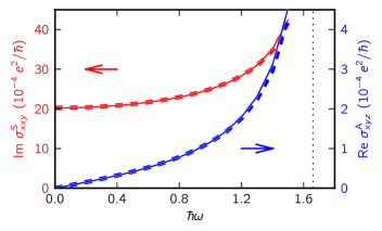
Figure 1: (Color online) The $xxy$ component of the gyrotropic birefringence tensor $\mathrm{Im}\,\sigma^{\mathrm{S}}_{abc}$, and the $xyz$ component of the natural optical activity tensor $\mathrm{Re}\,\sigma^{\mathrm{A}}_{abc}$, calculated for the tight-binding model described in the text as a function of frequency. Solid lines: extrapolation from calculations on finite crystallites. Dashed lines: calculations on periodic crystals using the $k$-space formulas derived in this work. The vertical dotted line indicates the frequency corresponding to the direct band gap.

In order to check the expressions derived in the previous section, we have carried out numerical tests comparing calculations done under periodic boundary conditions against reference calculations on finite crystallites. We chose for our tests the tight-binding model of Ref. malash2010, . This is a spinless model on a $2\times 2\times 2$ cubic lattice, where $\mathcal{P}$ symmetry is broken by assigning random on-site energies and $\mathcal{T}$ symmetry is broken by complex first-neighbor hoppings. The model parameters in Table A.1 of Ref. malash2010, were used (one of the complex hopping phases, labeled $\varphi$ therein, shall be used as a control parameter), and the two lowest bands were treated as occupied.

The tensor components $\mathrm{Im}\,\sigma^{\mathrm{S}}_{xxy}$ and $\mathrm{Re}\,\sigma^{\mathrm{A}}_{xyz}$ were evaluated at nonabsorbing frequencies. The calculations on periodic samples were done on a $30\times 30\times 30$ mesh of $k$ points using Eqs. (30)–(36), together with the sum-over-states formula for ${\bm{\nabla}}_{\bf k}|u_{n{\bf k}}\rangle$.malash2010 For the calculations on finite samples we used Eqs. (19) and (20),

$$\mathrm{Im}\,\sigma^{\mathrm{S}}_{xxy}=2c\mathrm{Re}\,\alpha_{xz}+\omega\mathrm{Im}\,\gamma_{xxy}\doteq 2c\alpha_{xz}-i\omega\gamma_{xxy}$$ (49)

and

$$\begin{split}\mathrm{Re}\,\sigma_{xyz}^{\mathrm{A}}&=-c\mathrm{Im}(\beta_{xx}+\beta_{yy})+\omega\mathrm{Re}\,\xi_{xyz}\\ &\doteq ic(\beta_{xx}+\beta_{yy})+\omega\xi_{xyz},\end{split}$$ (50)

together with Eqs. (21)–(24) and (52)–(55) for the magnetoelectric ($\alpha$, $\beta$) and quadrupolar ($\gamma$, $\xi$) tensors. We chose cubic samples containing $L\times L\times L$ unit cells, with $L=1,\,2,\,3,\,4$, and then extrapolated the calculated values to $L\rightarrow\infty$.malash2010

Figure 1 shows as solid (dashed) lines the frequency dependence of $\mathrm{Im}\,\sigma^{\mathrm{S}}_{xxy}$ and $\mathrm{Re}\,\sigma^{\mathrm{A}}_{xyz}$ for finite (periodic) samples, with the parameter $\varphi$ set to $\pi$. The natural optical activity spectrum starts off at zero and increases with frequency, exhibiting a resonant behavior as the minimum direct gap, denoted by the vertical dashed line, is approached. The ME optical spectrum displays a similar behavior, except that it remains finite as $\omega$ goes to zero. The excellent agreement between solid and dashed lines demonstrates the correctness of the $k$-space formulas.

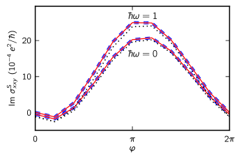
Figure 2: (Color online) The $xxy$ component of $\mathrm{Im}\sigma^{\mathrm{S}}_{abc}(\omega)$, calculated for the tight-binding model described in the text as a function of the parameter $\varphi$. Solid lines: extrapolation from calculations on finite crystallites using Eq. (49). Dashed lines: calculations on periodic crystals using Eqs. (30) and (31). Dotted lines: same as the dashed lines, but ommiting the contribution coming from Eq. (31).

Next we discuss a number of additional numerical tests where we investigate in more detail the behavior of $\mathrm{Im}\,\sigma^{\mathrm{S}}_{xxy}$. In these tests the frequency was kept fixed, and the parameter $\varphi$ was scanned over the range $[0,2\pi]$.

In Figure 2 we plot $\mathrm{Im}\,\sigma^{\mathrm{S}}_{xxy}$ versus $\varphi$ for two frequencies, $\omega=0$ and $\hbar\omega=1$. As before, solid and dashed lines represent calculations on finite and periodic samples respectively. In addition, we show as dotted lines the result of a periodic-sample calculation using only the matrix element (m) term, Eq. (30), i.e., omitting the energy (e) term, Eq. (31). We see that the energy term gives a small but visible contribution, which must be included in order to find agreement with the finite-sample calculation.

We now turn to the decomposition of $\mathrm{Im}\,\sigma^{\mathrm{S}}_{xxy}$ according to Eq. (49), into magnetoelectric and quadrupolar parts. They are plotted separately in Fig. 3 for $\hbar\omega=1$ and $L=4$. We chose a specific $L$ because $\alpha$ and $\omega\gamma$ are origin-dependent quantities, and it is therefore not meaningful to extrapolate them separately to $L\rightarrow\infty$. The dashed lines show how each of them changes when the position of the sample is shifted. The change in $\alpha_{zz}$ is exactly compensated by the change in $\omega\gamma_{xxy}$, so that the resulting $\mathrm{Im}\,\sigma^{\mathrm{S}}_{xxy}$ remains the same to machine precision, demonstrating its translational invariance.

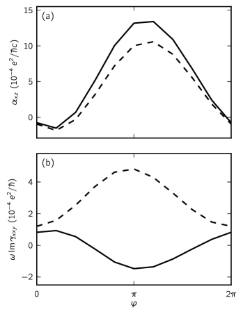
Figure 3: Origin-dependence of the bare magnetoelectric (upper panel) and quadrupolar (lower panel) polarizabilities appearing on the right-hand side of Eq. (49), calculated at $\hbar\omega=1$ for a finite sample ($L=4$) of the model used in Fig. 2. Solid lines: the center of the sample is placed at the origin. Dashed lines: the sample is displaced by $\mathbf{r}=(1,1,1)$, in units of the lattice constant of the $2\times 2\times 2$ cubic cell.

An alternative decomposition of $\mathrm{Im}\,\sigma^{\mathrm{S}}_{xxy}$ is given by Eq. (25):

$$\mathrm{Im}\,\sigma^{\mathrm{S}}_{xxy}\doteq 2c\widetilde{\alpha}_{xz}-i\omega\widetilde{\gamma}_{xxy}.$$ (51)

Unlike the bare property tensors $\alpha$ and $\omega\gamma$ appearing in Eq. (49), the renormalized magnetoelectriclike and purely quadrupolar tensors $\widetilde{\alpha}$ and $\omega\widetilde{\gamma}$ are origin independent and hence separately well defined for periodic samples. Figure 4 shows as dashed (solid) lines their values calculated for periodic (finite) samples from the first (second) equality in Eqs. (26) and (27). Because $\widetilde{\alpha}$ reduces to the traceless part of $\alpha$ as $\omega\rightarrow 0$, we can directly compare the curve for $\widetilde{\alpha}_{xz}(0)$ with a $k$-space calculation of $\alpha_{xz}(0)$ using the formula derived in Refs. malash2010, ; essin2010, (open circles). The precise agreement confirms numerically the analysis of Sec. III.2.

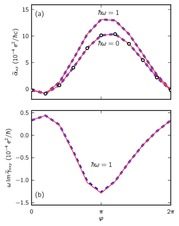
Figure 4: (Color online) Translationally invariant decomposition [Eq. (51)] of the curves in Fig. 2 into magnetoelectriclike (upper panel) and purely quadrupolar (lower panel) contributions. Solid lines: extrapolation from calculations on finite crystallites. Dashed lines: $k$-space calculations on periodic crystals. In the static limit the tensor $\widetilde{\alpha}$ reduces to the traceless part of the magnetoelectric polarizability $\alpha$, and the open circles show $\alpha_{xz}(0)$ calculated in $k$ space according to Refs. malash2010, ; essin2010, .

V Summary and outlook

In this work we investigated spatial-dispersion optical effects in insulators. The main result is a band-theory expression for $\sigma_{abc}(\omega)$, the spatially dispersive optical conductivity. Special attention was given to the ${\cal T}$-odd part of this tensor, which is nonzero in magnetoelectric crystals, and comprises magnetoelectriclike ($\widetilde{\alpha}_{ab}$) and purely quadrupolar ($\widetilde{\gamma}_{abc}$) contributions. We showed that each of them consists of a translationally invariant combination of separately origin dependent molecular polarizability tensors.

The magnetoelectriclike tensor $\widetilde{\alpha}_{ab}$ has both spin and orbital contributions, and the expression for the orbital part generalizes to finite frequencies the recently developed band theory of orbital magnetoelectric response.malash2010 ; essin2010 The generalization is, however, not complete, as the tensor $\widetilde{\alpha}_{ab}(\omega)$ is traceless, and therefore does not include the isotropic ME coupling. The reason why the latter is not recovered from the present formalism is that our starting point is the current response of an infinite medium to an electromagnetic wave while the trace of the ME tensor, known as the axion contribution, only affects electrodynamics at boundaries.hornreich68 ; essin2010 The calculation of the axion piece at finite frequencies remains an open problem.

The bulk expression for $\sigma_{abc}(\omega)$ at transparent frequencies was validated by performing numerical calculations on a tight-binding model, and comparing against reference calculations done on finite samples. The quantities needed to evaluate that expression are the occupied and empty energy eigenvalues and their $k$-space gradients, the off-diagonal Berry connection matrix Eq. (34), and the orbital and spin matrices Eqs. (36) and (37). The evaluation of all these objects in a first-principles context can be done efficiently by mapping the electronic structure onto localized Wannier orbitals, and then using the technique of Wannier interpolation.wang06 This approach has already been used to compute the magnetic circular dichroism spectrum of ferromagnets.yates07

First-principles calculations of the optical spectrum of solids beyond the electric-dipole approximation are still in their infancy. We hope that the formalism introduced in this work will be useful for carrying out realistic calculations of spatial-dispersion phenomena in the optical range, including natural optical activity, gyrotropic birefringence, and directional dichroism.

Appendix A Quantum-mechanical expressions for the polarizability tensors

In this appendix we list the quantum-mechanical expressions for the frequency-dependent polarizability tensors $\chi^{\rm em}$, $\chi^{\rm me}$, $\chi^{\rm q}$, and $\widetilde{{\chi}^{\rm q}}$ of bounded samples. They have been used to produce the reference results (solid lines) in Figs. 2–4.

We provide the single-particle version of the formulas in the lossless regime, which is the form used in Sec. IV. A many-body derivation can be found in Ref. raab2005, , and the modifications needed to describe absorption are discussed in Refs. barron2004, ; raab2005, .

Defining $Z_{ln}=(V\hbar/2e^{2})(\omega_{ln}^{2}-\omega^{2})$, where $V$ is the system volume, the orbital contribution to the magnetoelectric tensor reads

$$\mathrm{Re}\,\chi^{\mathrm{em}}_{ab}\doteq\frac{1}{2c}\sum_{n,l}^{o,e}\frac{\omega_{ln}}{Z_{ln}}\mathrm{Re}\,\bigl{[}\langle n|r_{a}|l\rangle\langle l|({\bf r}\times{\bf v})_{b}|n\rangle\bigr{]}\doteq\mathrm{Re}\,\chi^{\mathrm{me}}_{ba},$$ (52)

$$\mathrm{Im}\,\chi^{\mathrm{em}}_{ab}\doteq\frac{1}{2c}\sum_{n,l}^{o,e}\frac{\omega}{Z_{ln}}\mathrm{Im}\,\bigl{[}\langle n|r_{a}|l\rangle\langle l|({\bf r}\times{\bf v})_{b}|n\rangle\bigr{]}\doteq-\mathrm{Im}\,\chi^{\mathrm{me}}_{ba}$$ (53)

and the quadrupolar polarizability reads

$$\mathrm{Re}\,\chi^{\rm q}_{abc}\doteq\sum_{n,l}^{o,e}\frac{\omega_{ln}}{Z_{ln}}\mathrm{Re}\,\bigl{[}\langle n|r_{a}|l\rangle\langle l|r_{b}r_{c}|n\rangle\bigr{]}\doteq\mathrm{Re}\,\widetilde{{\chi}^{\rm q}}_{cba},$$ (54)

$$\mathrm{Im}\,\chi^{\rm q}_{abc}\doteq\sum_{n,l}^{o,e}\frac{\omega}{Z_{ln}}\mathrm{Im}\,\bigl{[}\langle n|r_{a}|l\rangle\langle l|r_{b}r_{c}|n\rangle\bigr{]}\doteq-\mathrm{Im}\,\widetilde{{\chi}^{\rm q}}_{cba}.$$ (55)

Appendix B Derivation of Eq. (47)

In order to derive Eq. (47), we drop the spin contribution, Eq. (37), from Eqs. (30) and (31) and rewrite the orbital contribution at $\omega=0$ as

$$\mathrm{Im}\,\sigma^{({\rm orb})}_{{\rm S},abc}(0)=\frac{e^{2}}{\hbar}\int[d{\bf k}]\left[(C_{abc}+D_{abc})+(C_{bac}+D_{bac})\right],$$ (56)

where

$$\begin{split}C_{abc}=\sum_{n,l}^{o,e}\mathrm{Re}\biggl{\{}\frac{\langle u_{l}|\partial_{b}u_{n}\rangle}{E_{l}-E_{n}}\Bigl{[}\langle u_{n}|(\partial_{a}H)|\partial_{c}u_{l}\rangle-\\ \langle\partial_{c}u_{n}|(\partial_{a}H)|u_{l}\rangle\Bigr{]}\biggr{\}}\end{split}$$ (57)

and

$$D_{abc}=\sum_{n,l}^{o,e}\frac{\partial_{c}(E_{l}+E_{n})}{E_{l}-E_{n}}\mathrm{Re}\{\langle\partial_{a}u_{n}|u_{l}\rangle\langle u_{l}|\partial_{b}u_{n}\rangle\}.$$ (58)

We will use repeatedly the identitymalash2010

$$\partial_{c}(H-E_{l})|u_{l}\rangle=(E_{l}-H)|\partial_{c}u_{l}\rangle,$$ (59)

as well as the following expression for the field derivative of a valence-band state projected onto the conduction bandsmalash2010

$$|\widetilde{\partial}_{\mathcal{E}_{b}}u_{n}\rangle=-ie\sum_{l}^{e}\frac{|u_{l}\rangle\langle u_{l}|}{E_{l}-E_{n}}|\partial_{b}u_{n}\rangle.$$ (60)

We start by using Eq. (59) to eliminate $\partial_{c}E_{l}$ from Eq. (58),

$$\begin{split}D_{abc}&=\sum_{n,l}^{o,e}\mathrm{Re}\biggl{\{}\frac{\langle\partial_{a}u_{n}|(\partial_{c}H)|u_{l}\rangle\langle u_{l}|\partial_{b}u_{n}\rangle}{E_{l}-E_{n}}\\ &+\frac{\langle\partial_{a}u_{n}|H-E_{l}|\partial_{c}u_{l}\rangle\langle u_{l}|\partial_{b}u_{n}\rangle}{E_{l}-E_{n}}\\ &+\frac{\partial_{c}E_{n}}{E_{l}-E_{n}}\langle\partial_{a}u_{n}|u_{l}\rangle\langle u_{l}|\partial_{b}u_{n}\rangle\biggr{\}}\end{split}$$ (61)

and then use Eq. (60) twice to find

$$\begin{split}D_{abc}=-\frac{1}{e}\sum_{n}^{o}\mathrm{Im}\langle\partial_{a}u_{n}|\partial_{c}(H+E_{n})|\widetilde{\partial}_{\mathcal{E}_{b}}u_{n}\rangle\\ +\sum_{n,l}^{o,e}\mathrm{Re}\left\{\frac{\langle\partial_{a}u_{n}|H-E_{l}|\partial_{c}u_{l}\rangle\langle u_{l}|\partial_{b}u_{n}\rangle}{E_{l}-E_{n}}\right\}.\end{split}$$ (62)

Now write $H-E_{l}$ as $(H-E_{n})+(E_{n}-E_{l})$ and use Eq. (59),

$$\begin{split}D_{abc}&=T_{abc}-\frac{1}{e}\sum_{n}^{o}\mathrm{Im}\langle\partial_{a}u_{n}|\partial_{c}(H+E_{n})|\widetilde{\partial}_{\mathcal{E}_{b}}u_{n}\rangle\\ &+\sum_{n,l}^{o,e}\mathrm{Re}\left\{\frac{\langle u_{n}|\partial_{a}(E_{n}-H)|\partial_{c}u_{l}\rangle\langle u_{l}|\partial_{b}u_{n}\rangle}{E_{l}-E_{n}}\right\},\end{split}$$ (63)

where we defined

$$T_{abc}=-\sum_{n,l}^{o,e}\mathrm{Re}\langle\partial_{a}u_{n}|\partial_{c}u_{l}\rangle\langle u_{l}|\partial_{b}u_{n}\rangle.$$ (64)

One term in Eq. (63) exactly cancels the first term in Eq. (57). For the remainder we use $\langle u_{n}|\partial_{c}u_{l}\rangle=-\langle\partial_{c}u_{n}|u_{l}\rangle$ once and then Eq. (60) twice, yielding

$$\begin{split}&C_{abc}+D_{abc}=T_{abc}\\ &+\frac{1}{e}\sum_{n}^{o}\mathrm{Im}\left\{\langle\partial_{c}u_{n}|\partial_{a}(H+E_{n})|\widetilde{\partial}_{\mathcal{E}_{b}}u_{n}\rangle-a\leftrightarrow c\right\}.\end{split}$$ (65)

In order to eliminate the sum over empty states in $T_{abc}$ we need to combine $C_{abc}+D_{abc}$ with $C_{bac}+D_{bac}$, as in Eq. (56). We therefore consider

$$\begin{split}T_{abc}+T_{bac}&=-\sum_{n,l}^{o,e}\mathrm{Re}\Bigl{\{}\langle\partial_{a}u_{n}|\partial_{c}u_{l}\rangle\langle u_{l}|\partial_{b}u_{n}\rangle+a\leftrightarrow b\Bigr{\}}\\ &=-\sum_{n}^{o}\mathrm{Re}\Bigr{\{}\langle\partial_{a}u_{n}|(\partial_{c}Q)|\partial_{b}u_{n}\rangle\Bigl{\}}\\ &=\sum_{nm}^{o}\mathrm{Re}\Bigr{\{}\langle\partial_{a}u_{n}|\partial_{c}u_{m}\rangle\langle u_{m}|\partial_{b}u_{n}\rangle\\ &\;\;\;\;\;\;\;\;\;\;\;\;\;+\langle\partial_{b}u_{n}|\partial_{c}u_{m}\rangle\langle u_{m}|\partial_{a}u_{n}\rangle\Bigl{\}},\end{split}$$ (66)

where $Q=\sum_{l}^{e}|u_{l}\rangle\langle u_{l}|=1-\sum_{m}^{o}|u_{m}\rangle\langle u_{m}|$. Collecting terms, we arrive at Eq. (47).

References

- (1) T. Arima, J. Phys.: Condens. Matter 20, 434211 (2008)
- (2) W. F. Brown, S. Shtrikman, and D. Treves, J. Appl. Phys. 34, 1233 (1963)
- (3) B. B. Krichevtsov, V. V. Pavlov, R. V. Pisarev, and V. N. Gridnev, J. Phys.: Condens. Matter 5, 8233 (1993)
- (4) R. M. Hornreich and S. Shtrikman, Phys. Rev. 171, 1065 (1968)
- (5) L. D. Landau and E. M. Lifshitz, Electrodynamics of Continuous Media (Elsevier, 1984)
- (6) L. D. Barron, Molecular Light Scattering and Optical Activity (Cambridge University Press, Cambridge, 2004)
- (7) R. E. Raab and O. L. De Lange, Multipole Theory in Electromagnetism (Clarendon Press, Oxford, 2005)
- (8) K. Natori, J. Phys. Soc. Jpn. 39, 1013 (1975)
- (9) H. Zhong, Z. H. Levine, D. C. Allan, and J. W. Wilkins, Phys. Rev. Lett. 69, 379 (1992)
- (10) H. Zhong, Z. H. Levine, D. C. Allan, and J. W. Wilkins, Phys. Rev. B 48, 1384 (1993)
- (11) V. N. Muthukumar, R. Valenti, and C. Gros, Phys. Rev. B 54, 433 (1996)
- (12) J.-I. Igarashi and T. Nagao, Phys. Rev. B 80, 054418 (2009)
- (13) E. I. Blount, in Solid State Physics, Vol. 13, edited by F. Seitz and D. Turnbull (Academic, New York, 1962)
- (14) R. D. King-Smith and D. Vanderbilt, Phys. Rev. B 47, 1651 (1993)
- (15) R. Resta and D. Vanderbilt, in Physics of Ferroelectrics: A Modern Perspective, edited by K. M. Rabe, C. H. Ahn, and J.-M. Triscone (Springer-Verlag, Berlin, 2007) pp. 31–68
- (16) T. Thonhauser, D. Ceresoli, D. Vanderbilt, and R. Resta, Phys. Rev. Lett. 95, 137205 (2005)
- (17) D. Xiao, J. Shi, and Q. Niu, Phys. Rev. Lett. 95, 137204 (2005)
- (18) D. Ceresoli, T. Thonhauser, D. Vanderbilt, and R. Resta, Phys. Rev. B 74, 024408 (2006)
- (19) J. Shi, G. Vignale, D. Xiao, and Q. Niu, Phys. Rev. Lett. 99, 197202 (2007)
- (20) A. Malashevich, I. Souza, S. Coh, and D. Vanderbilt, New J. Phys. 12, 053032 (2010)
- (21) A. M. Essin, A. M. Turner, J. E. Moore, and D. Vanderbilt, Phys. Rev. B 81, 205104 (2010)
- (22) D. B. Melrose and R. C. McPhedran, Electromagnetic Processes in Dispersive Media (Cambridge University Press, Cambridge, 1991)
- (23) This can be seen by expanding in the Onsager reciprocity relationlandau ; melrose , where denotes the magnetic order parameter of the medium.
- (24) C. Train, R. Gheorghe, V. Krstic, L.-M. Chamoreau, N. S. Ovanesyan, G. L. J. A. Rikken, M. Gruselle, and M. Verdaguer, Nature Mater. 7, 729 (2008)
- (25) A. D. Buckingham and M. B. Dunn, J. Chem. Soc. A, 1988(1971)
- (26) W. A. Harrison, Solid State Theory (Dover, New York, 1980)
- (27) The optical activity of noncentrosymmetric metals was recently studied theoretically by V. P. Mineev and Yu. Yoshioka, Phys. Rev. B 81, 094525 (2010).
- (28) X. Wang, J. R. Yates, I. Souza, and D. Vanderbilt, Phys. Rev. B 74, 195118 (2006)
- (29) J. R. Yates, X. Wang, D. Vanderbilt, and I. Souza, Phys. Rev. B 75, 195121 (2007)