The effects of fly-bys on planetary systems

Abstract

Most of the observed extrasolar planets are found on tight and often eccentric orbits. The high eccentricities are not easily explained by planet-formation models, which predict that planets should be on rather circular orbits. Here we explore whether fly-bys involving planetary systems with properties similar to those of the gas giants in the solar system, can produce planets with properties similar to the observed planets. Using numerical simulations, we show that fly-bys can cause the immediate ejection of planets, and sometimes also lead to the capture of one or more planets by the intruder. More common, however, is that fly-bys only perturb the orbits of planets, sometimes leaving the system in an unstable state. Over time-scales of a few million to several hundred million years after the fly-by, this perturbation can trigger planet-planet scatterings, leading to the ejection of one or more planets. For example, in the case of the four gas giants of the solar system, the fraction of systems from which at least one planet is ejected more than doubles in $10^{8}$ years after the fly-by. The remaining planets are often left on more eccentric orbits, similar to the eccentricities of the observed extrasolar planets. We combine our results of how fly-bys affect solar-system-like planetary systems, with the rate at which encounters in young stellar clusters occur. For example, we measure the effects of fly-bys on the four gas giants in the solar system. We find, that for such systems, between 5 and 15 per cent suffer ejections of planets in $10^{8}$ years after fly-bys in typical open clusters. Thus, encounters in young stellar clusters can significantly alter the properties of any planets orbiting stars in clusters. As a large fraction of stars which populate the solar neighbourhood form in stellar clusters, encounters can significantly affect the properties of the observed extrasolar planets.

1 Introduction

More than 470 planets have been discovered since the first discovery of an extrasolar planet around a main-sequence star (Mayor & Queloz, 1995). The properties of most of these planets are very different from our solar system, with gas-giant planets on often much tighter and more eccentric orbits than seen in the solar system (http://www.exoplanet.eu). It is estimated that around 10 per cent of solar mass stars host gas-giant planets on orbits with semi-major axes less than 5 au (Cumming et al., 2008). In particular, the large spread in eccentricities poses a problem for planet formation, which is believed to occur in discs around young stars (see, for example, Pollack et al., 1996; Boss, 1997). This process will tend to leave planets on almost circular orbits.

It is today commonly believed that the observed eccentricities are caused by so-called planet-planet scattering, first discussed in Rasio & Ford (1996). Several models have been suggested to explain why planetary systems undergo such scattering. Moorhead & Adams (2008) suggest that systems containing two giant planets, which are migrating in a protoplanetary disc, can perturb each other’s orbits, exciting eccentricities. Such systems are unstable and often result in the removal of one planet due to ejection, collision or accretion onto the host star. The remaining planet is left on an eccentric orbit after the gas disc has dispersed.

It is however also possible that planetary systems evolve past the disc phase without undergoing scattering. If the planets are too tightly packed, such systems may become unstable on time-scales of a few to several 10 million years (e.g. Jurić & Tremaine, 2008; Ford & Rasio, 2008; Chatterjee et al., 2008; Raymond et al., 2009). While planet-planet scattering in these types of systems can explain the observed eccentricities, migration is needed to explain the observed semi-major axes (see, for example, Matsumura et al., 2010).

A somewhat different mechanism to explain the onset of planet-planet scattering in planetary systems is that they are triggered by encounters in the birth environment of many stars; stellar clusters. In such clusters, the high number density of stars causes encounters between stars to be common. So-called exchange encounters can leave planet-hosting stars, which formed single, in inclined binaries where the so-called Kozai mechanism can operate (Kozai, 1962). This can increase planetary eccentricities, particularly the eccentricity of the outermost planet, potentially triggering planet-planet scattering in multi-planet systems (Malmberg et al., 2007; Malmberg & Davies, 2009). However, depending on the binary fraction in stellar clusters, fly-bys may be much more common than exchange encounters. Essentially, in clusters with a high binary fraction, exchange encounters are likely to dominate, while in clusters with a low binary fraction, fly-bys are likely play the most important role. Fly-bys can, if they occur during the protoplanetary disc stage, change the frequency of planet formation (Forgan & Rice, 2009) or the orbital and physical properties of planets formed (Fragner & Nelson, 2009).

Fly-bys occurring after the stage of giant planet formation can excite eccentricities in planetary systems (Zakamska & Tremaine, 2004) and trigger planet-planet scattering in relatively packed systems (Spurzem et al., 2009).

Young stellar clusters also contain many young massive stars, whose strong radiation can damage protoplanetary discs (e.g. Armitage, 2000; Adams et al., 2006). Our understanding of the birth environment of the solar system was recently reviewed by Adams (2010). For example, the orbital elements of Sedna, along with the chemical composition of objects in the solar system, suggest that the Sun formed in a cluster with roughly $10^{3}$-$10^{4}$ stars.

In this paper we measure the effects of fly-bys on planetary systems resembling the solar-system, i.e. systems with gas giants on initially well-spaced and circular orbits. The effects of such fly-bys on both individual planetary systems, as well as on the population of planetary systems as a whole, can be significant. Below we summarise the most important findings from our experiments.

1. Close fly-bys can lead to the immediate ejection of one or more planets from the host system (see also Hills, 1984; Hurley & Shara, 2002; Fregeau et al., 2006; Spurzem et al., 2009). Such planets may either be left unbound (ionisation), or be captured by the intruder star (exchange). We measure what fraction of fly-bys that causes ionisation and exchange to occur in Section 3, and in Table 5 we present the rates at which such encounters occur in stellar clusters with properties representative of the young cluster population in the solar neighbourhood. For example, in a cluster with initially 700 stars and half-mass radius of 0.38 pc, 3 per cent of stars hosting a planetary system similar to the four gas giants of the solar system will suffer a fly-by leading to the immediate removal of one or more planets from the host star.

2. Wider fly-bys, which do not immediately remove planets from the host star, may still cause the ejection of planets on longer time scales. As shown in section 4, the fraction of planetary systems from which at least one planet is ejected more than doubles in the $10^{8}$ years following a stellar encounter. These later ejections are caused by planet-planet scattering, triggered because the fly-by increased the eccentricities of the planets (see also Zakamska & Tremaine, 2004), and/or changed their semi-major axes, leaving the system in an unstable configuration.

3. If the intruder in a fly-by is a low-mass star, or even a brown dwarf, an exchange reaction may occur, similar to what is seen for stellar binaries in clusters (e.g. Heggie, 1975). The intruder may then become bound to the host star, significantly increasing the effect of such fly-bys on planetary systems. We have done a large set of scattering simulations of encounters between planetary systems and low-mass intruders, and find that such encounters can play an important role in the evolution of planetary systems in stellar clusters. This shows that a more detailed study of such encounters is warranted and we will present that in a forthcoming paper.

4. In general, fly-bys excite the eccentricities of planets, both through direct scattering off the intruder, and through any subsequent planet-planet scattering. We find that the eccentricity distribution of planets which have been scattered onto orbits tighter than 4.5 au in fly-bys involving planetary systems that initially resembles the solar system, is similar to that of the observed extrasolar planets (see Fig. 7 and discussion in section 9.2). It is important to note that varying the initial properties of the planetary systems will significantly affect the properties of the systems post scattering (see also Jurić & Tremaine, 2008; Raymond et al., 2009). We explore this further in section 6 and 7.

5. Planet-planet scattering decreases the semi-major axes of one or more planets, while leaving others on either much wider orbits or ejected. However, planet-planet scattering in systems resembling the solar system, with gas giants initially on orbits of 5 au or wider, can only decrease the semi-major axis of the inner planet by roughly a factor of two. Hence, the semi-major axes distribution of such post-scattering systems does not match the observed distribution. Planet-planet scattering models thus need a contribution from planetary systems with planets on initially tighter orbits than those of the gas giants in the solar system in order to reproduce both the observed semi-major axes and eccentricity distributions. Hence, disc migration, occurring before the stellar encounter, is needed to explain the observed semi-major axes (see, for example, Matsumura et al., 2010).

6. During planet-planet scattering, one or more planets are successively scattered onto wider and wider orbits, until they become unbound. The remaining planets are scattered onto tighter orbits (Scharf & Menou, 2009; Veras et al., 2009). During this phase it may be possible to observe planets on very wide orbits using imaging techniques. It is important to note that this behaviour is independent of what mechanism triggered the planet-planet scattering. As such, fly-by induced planet-planet scattering will produce planets on wide orbits. Furthermore, planets which are captured by the intruder stars in fly-bys are often left on rather wide orbits, and thus could be observed in imaging surveys. We explore both these mechanisms in Section 8.

In Section 2 we review the encounter rates in young open clusters, measured using $N$-body simulations (Malmberg et al., 2007). In particular, we discuss the rate of fly-bys involving solar-mass stars, as these are most applicable to solar-system-like planetary systems.

In Section 3, we describe the properties of planetary systems immediately after a fly-by, as measured through both numerical simulations and analytical calculations. We measure the fraction of systems from which planets are immediately ejected, and the rate at which planets are captured by the intruder star. We also measure how important relatively distant fly-bys are in terms of moderately exciting the inclinations and eccentricities of planetary systems.

We describe the evolution of the four gas-giants of the solar system after a fly-by in Section 4. For example, we measure the fraction of such systems in which planet-planet scattering is triggered within $10^{8}$ years after the fly-by. We also discuss the possibility of predicting the future evolution of such systems immediately after the fly-by.

In Section 5 we measure the rate at which low-mass intruders are captured in encounters with planetary systems, and discuss the implications such encounters may have on the future evolution of the system.

We proceed to measure the post-fly-by evolution of planetary systems slightly different from the solar system. In section 7 we go through the effects of fly-bys on systems similar to the four gas giants, but where we have changed the masses of the planets. In section 8 we simulate the evolution after a fly-by, of a planetary system consisting of 5 gas-giants, generated in simulations of planet formation by Levison et al. (1998).

In section 9 we combine the encounter rates in stellar clusters, with the measured effects of fly-bys, to understand the effect on the population of planets in clusters of different sizes. We also describe some of the properties of this population.

In section 10, we discuss the implications of encounters where the intruding star is in fact an intruding binary. We do not consider the effect of such encounters here. In our simulations of stellar clusters (Malmberg et al., 2007) we had a relatively low primordial binary fraction, and as such these encounters are not frequent. If we were to increase the primordial binary fraction, however, we would see many more such encounters, and we discuss how this would affect our results. We also, for example, review some of the effects of fly-bys on protoplanetary discs, and discuss how changing the primordial binary fraction in our clusters can affect our results. We summarise our results in section 11.

2 Close encounter rates in young stellar clusters

In this section we review our simulations of stellar clusters, and describe the encounter rates of solar-mass stars.

2.1 Cluster properties

We have performed a large set of N-body simulations of young stellar clusters, with properties representative of the open cluster population in the solar neighbourhood (see Malmberg et al., 2007, for more details). We used the publicly available package NBODY6, which is a full force-summation direct $N$-body code. A complete description of the physics included and algorithms used in NBODY6 can be found in Aarseth (2003). During the simulations, we measured the encounter rates of stars and binaries, focussing especially on fly-bys and so-called exchange encounters. In our simulations we define a fly-by as when two stars pass each other with in a minimum separation of $r_{\rm min}<1000\,\mbox{au}.$ In an exchange encounter, a single star encounters a binary system and replaces one of the stars in the binary.

In our simulations we consider the evolution of the stellar clusters after the removal of the primordial gas initially present in the cluster. The properties of the clusters were chosen so as to represent the observed open clusters in the solar neighbourhood. At least 10 per cent of stars form in such clusters, while the remaining form either in clusters which disperse due to gas removal or in small groups or associations (e.g. van den Bergh, 1981; Elmegreen & Clemens, 1985; Battinelli & Capuzzo-Dolcetta, 1991; Adams & Myers, 2001). Clusters which survive the loss of primordial gas nevertheless disperse; our simulated clusters have lifetimes of between 400 and 1100 million years.

In this paper, we consider clusters with an initial half-mass radius, $r_{\rm h}=0.38$ pc and an initial number of stars of $N=150,300,500,700$ and $1000$ respectively. In all these simulations, one third of stars were in primordial binaries. The stellar masses were drawn from the initial mass function of Kroupa et al. (1993) with a lower mass of $0.2M_{\odot}$ and upper mass of $5M_{\odot}$. The initial positions of the stars were chosen such that their distribution followed the spherically symmetric Plummer (1911) model:

$$\rho(\mathbf{r})=\frac{3M_{\rm cl}}{4\pi r^{3}_{0}}\frac{1}{[1+(r/r_{0})^{2}]^{5/2}},$$ (1)

for total cluster mass $M_{\rm cl}$. Here, $r_{0}$ is a constant, which is connected to the half-mass radius of the cluster as (Heggie & Hut, 2003): $r_{\rm h}\approx 1.305r_{0}$.

For each particular cluster type, we performed 10 realisations, performing a new draw from the IMF and generating a new set of initial positions and velocities for each realisation.

2.2 Encounter rates

In Fig. 1 we show the fractions of initially single stars that underwent fly-bys and/or exchange encounters in the cluster with $N=700$. The results are averaged over 10 realisations. The cluster quickly expanded from its initial half-mass radius of $r_{\rm h}=0.38$ pc to $r_{\rm h}\sim 2$ pc, whereafter $r_{\rm min}$ was roughly constant for the remaining lifetime of the cluster. From now on, we will refer to this cluster as our reference cluster. The circle labelled B contains the stars which spent some time in a binary during the cluster’s lifetime, the circle labelled F contains those stars which underwent a fly-by with other stars. Finally, the circle labelled S contains those stars which were single at the end of the cluster’s lifetime. About 6.5 per cent of the initially single stars spent time inside a binary system, while about 73.5 per cent underwent a at least one fly-by with another star. About 20 per cent of the initially single stars did not spend time inside a binary or undergo a fly-by. We call such stars singletons. A singleton is defined by us as:

1. a star which has not formed in a binary,

2. a star which has not later spent time within a binary system,

3. a star which has not suffered close encounters with other stars.

A planetary system orbiting a star that is not a singleton may have had its evolution changed due to interactions with other stars.

In Fig. 2 we show the interaction rates in our reference cluster (same cluster as in Fig. 1), but now only for stars with $0.8\,M_{\odot}<m<1.2\,M_{\odot}$. As can be seen in the figure, the fraction of initially single stars which remain singletons throughout the lifetime of the cluster is lower for solar-mass stars; only about 15 per cent. The fraction of solar-mass stars which spend some time within a binary system is roughly similar, while the fraction which have undergone at least one fly-by is higher (78 per cent). This increase in the frequency of interactions is due in part to the effects of mass segregation, which draws the heavier solar-like stars into the denser central regions of the cluster.

In Fig. 3 we plot the distribution of the number of fly-bys experienced, $n_{\rm fb}$, for the initially-single solar-mass stars that have undergone fly-bys in our reference cluster. About 75 per cent of them have experienced two or more fly-bys. The mean number of fly-bys per star is in fact four. Stars which have undergone several fly-bys will, on average, have closer encounters with other stars than systems only undergoing a single flyby. The cross section for two stars, having a relative velocity at infinity of $v_{\infty}$, to pass within a minimum distance $r_{\rm min}$ is given by

$$\sigma=\pi r_{\rm min}^{2}\left(1+{v^{2}\over v_{\infty}^{2}}\right)$$ (2)

where $v$ is the relative velocity of the two stars at closest approach in a parabolic encounter i.e.  $v^{2}=2G(m_{1}+m_{2})/r_{\rm min}$, where $m_{1}$ and $m_{2}$ are the masses of the two stars. The second term is due to the attractive gravitational force, and is referred to as gravitational focussing. In the regime where $v\ll v_{\infty}$ (as might be the case in galactic nuclei with extremely high velocity dispersions), we recover the result, $\sigma\propto r_{\rm min}^{2}$. However, if $v\gg v_{\infty}$ as will be the case in systems with low velocity dispersions, such as young clusters, $\sigma\propto r_{\rm min}$. Thus a star that has had a number of fly-bys, $n_{\rm fb}$, within 1000 au will on average have passed within a mean minimum distance, ${\langle r_{\rm min}\rangle}_{\rm min}$, of:

$${\langle r_{\rm min}\rangle}_{\rm min}=1000\,\mbox{au}/n_{\rm fb}.$$ (3)

As the mean number of fly-bys in our reference cluster is four, we thus find ${\langle r_{\rm min}\rangle}_{\rm min}=250$ au.

In Fig. 4 we plot the distribution of when fly-bys occur, $t_{\rm fb}$ ($r_{\rm min}<1000$ au) as a function of cluster age. As can be seen in the figure, the evolution is very similar for all clusters. On average, half of the fly-bys occur within the first 10 million years This time-scale is in principle comparable to the gas-giant planet formation time-scale, but as our simulations only treat the post-gas-loss life of clusters, gas-giant planets have already formed at the start of our simulations.

Figure 1: Venn diagram of the stars which were initially single in our reference cluster ($N=700$ and $r_{\rm h,initial}=0.38$ pc). The numbers are the average result from 10 realisations. The upper circle contains stars which were single at the end of the run (S), the lower left-hand circle contains the stars which were in a bound system (i.e. triple or binary) during the lifetime of the cluster (B) and the lower right-hand circle contains the stars which had experienced a fly-by (F) (defined as when two stars pass within 1000 au of each other).

Figure 2: Venn diagram of the stars which were initially single in our reference cluster ($N=700$ and $r_{\rm h,initial}=0.38$ pc) and had mass between $0.8M_{\odot}$ and $1.2M_{\odot}$ . The numbers are the average result from 10 realisations. The upper circle contains stars which were single at the end of the run (S), the lower left-hand circle contains the stars which were in a bound system (i.e. triple or binary) during the lifetime of the cluster (B) and the lower right-hand circle contains the stars which had experienced a fly-by (F) (defined as when two stars pass within 1000 au of each other).

Figure 3: The distribution of number of fly-bys, $n_{\rm fly-bys}$, per star for the initially single stars with mass $0.8<m<1.2M_{\odot}$ that experienced fly-bys in our reference cluster ($N=700$ and $r_{\rm h,initial}=0.38$ pc). The average number of fly-bys per star in the cluster is 4.

Figure 4: The fraction of all encounters which have occurred as function of cluster age, averaged over the 10 realisations for each cluster. Only clusters with initial half-mass radii of 0.38 pc are included. These clusters have radii of about 2-4 pc during most of their lifetime.

3 The properties of planetary systems immediately after a fly-by

We begin here by describing in detail the effects of fly-bys on a planetary system consisting of the four gas-giant planets of the solar system (4G). The immediate effect of a fly-by depends crucially on the minimum separation between the intruder star and the planetary-system-host star during the encounter, $r_{\rm min}$. We divide fly-bys into two different regimes, depending on $r_{\rm min}$; the strong regime ($r_{\rm min}<100$ au) and the the weak regime ($100<r_{\rm min}<1000$ au).

To analyse the encounters we use a combination of direct numerical simulations (in the strong regime) and analytic theory (in the weak regime). In all our simulations, we set the relative velocity of the two stars, $v_{\infty}=1$ km/s, which is the typical velocity dispersion in young stellar clusters.

To perform the numerical simulations, we use the Bulirsch–Stoer algorithm, as implemented in the MERCURY6 package (Chambers, 1999).

3.1 The strong regime: $r_{\rm min}<100$ au

Figure 5: The probability that no planets are ejected or captured (thin lines) and that one planet is captured by the intruder star (thick lines) immediately after the fly-by as a function of $r_{\rm min}$ for encounters involving the four gas giants. The solid lines are for encounters where $m_{\rm I}=0.6M_{\odot}$, the long-dashed lines are for encounters where $m_{\rm I}=1.0M_{\odot}$ and the short-dashed lines are for encounters where $m_{\rm I}=1.5M_{\odot}$.

Close fly-bys cause significant changes in the orbits of planets. Often, they lead to the immediate ejection of planets or an exchange, in which planets become bound to the intruder star. We have performed $6\times 10^{5}$ scattering experiments of fly-bys involving the four gas-giant planets of the solar system, with $r_{\rm min}<100$ au and intruder-star mass, $m_{\rm I}=0.6,1.0$ and $1.5M_{\odot}$.

In Fig. 5 we plot the probability that four planets remain bound to the host star immediately after the fly-by (thin lines) and the probability that one planet is captured by the intruder star (thick lines), as a function of $r_{\rm min}$. The semi-major axis of the outermost planet, Neptune, is 30 au. The probability that all four planets remain bound to the intruder star (thin lines) reaches unity at between two and three times the semi-major axis of the outermost planet, depending on the mass of the intruder star. For example, in fly-bys with $r_{\rm min}<100$ au and $m_{\rm I}=0.6M_{\odot}$, 15 per cent of fly-bys lead to one or more planets becoming unbound from the host star. Hence, in fly-bys where $r_{\rm min}$ is comparable in size to the semi-major axes of the planets’ orbits, the result is often to immediately unbind one or more planets. Sometimes planets are ejected from the system and left as free-floating planets, but it is not uncommon that planets instead are captured by the intruder star, and hence orbit it after the fly-by. In the latter case, the most likely outcome is that only one planet is captured (thick lines in Fig. 5).

3.2 The weak regime: $100<r_{\rm min}<1000$ au

Figure 6: The eccentricities of the the four gas giants of the solar system as function of number of fly-bys, $n_{\rm fb}$. The minimum separation between the host star and the intruder star was chosen randomly between 100 and 1000 au.

In encounters with $r_{\rm min}>100$ au we can measure the change in eccentricities and inclinations of the planets analytically (Heggie & Rasio, 1996). Three different cases must be considered, depending on the initial eccentricity of the planet (circular or eccentric) and on $r_{\rm min}$.

We have calculated the the average change in the eccentricity of the gas giant planets in the solar system with number of fly-bys, $n_{\rm fb}$ using equation (20), (21) and (23) from Appendix A. We assume that the intruder is randomly oriented with respect to the planets and has $m_{\rm I}=1.0M_{\odot}$. We plot the result in Fig. 6. A large number of fly-bys is required to significantly change the mean eccentricities of the planets. Also, as the cross-section for encounters scales with $r_{\rm min}$, a star will experience at least one encounter with $r_{\rm min}<100$ au for every 10 encounters it experiences with $100<r_{\rm min}<1000$ au. It is thus unlikely that fly-bys in the weak regime trigger planet-planet scatterings in planetary system similar to the solar system. They can, however, be important as a “heating mechanism” of planetary systems. For example, if we assume that the solar system initially started out circular and co-planar, we can ask the question “How many fly-bys, $n_{\rm fb}$ would be required to increase the values of the planets’ eccentricities and inclinations to their current values?” A complication here is that planet-planet interactions work to transfer angular momentum between planets, continuously changing the eccentricities and inclinations of the planets. Hence, any change in the inclination and eccentricities of the planets will propagate through the system (see, for example, Zakamska & Tremaine, 2004).

To estimate the number of fly-bys, $n_{\rm fb}$, required to take an initially co-planar and circular version of the solar system and give it similar eccentricities and inclinations to the present day solar system, we have chosen to calculate the so-called angular momentum deficit of the system, as a function of $n_{\rm fb}$.

The angular momentum deficit (AMD) in a system is the additional angular momentum present in it due to the non-circularity and non-co-planarity of the planetary orbits. It can be thought of as the amount of non-linearity present in the system. It is defined as (Laskar, 2000):

$$AMD=\sum^{n_{\rm p}}_{k=1}\Lambda_{\rm k}(1-\sqrt{1-e_{\rm k}^{2}}\cos{i_{\rm k}})$$ (4)

where $e_{\rm k}$ and $i_{\rm k}$ are the eccentricity and inclination of the $k^{\rm th}$ planet, and $\Lambda=m_{\rm k}\sqrt{\mu a_{\rm k}}$, where $m_{\rm k}$ and $a_{\rm k}$ are the mass and semi-major axis of the $k$th planet. Starting out with a co-planar system with planets on initially circular orbits we find that 15 fly-bys with solar-mass intruders with $100<r_{\rm min}<1000$, is enough to give the system its present AMD value.

4 Post-encounter evolution of planetary systems

Figure 7: The evolution of the four gas giants of the solar system, after a fly-by with $r_{\rm min}<100$ au. The periastron passage of the intruder star occurred at $t=0$. In panel a) we plot the fraction of systems, $f(t_{\rm eject}$), from which at least one planet has been ejected within, $t_{\rm eject}$ years after the fly-by and in panel b) we plot the fraction of systems, $f(t_{\rm encounter}$), in which at least two planets have passed within one mutual Hill radius of each other as a function of time, $t_{\rm encounter}$ after the fly-by.

Table 1: Overview of the evolution of the four gas giants of the solar system after a fly-by, divided into different categories depending on the state of the system immediately after the fly-by. In column 2 we list the categories and in column 3 we list the fraction of all systems which belongs to a given category. In column 4, 5, 6 and 7 we divide the systems from each category into four bins, depending on at what time after the fly-by the first planet was ejected from the system, $t_{\rm eject}$. In column 4 are systems with $t_{\rm eject}<10$ Myr, in column 5 systems with $t_{\rm eject}<30$ Myr, in column 6 systems with $t_{\rm eject}<100$ Myr and in column system are systems from which no planet was ejected in $10^{8}$ years. Its worth pointing out, that for systems in which a planet is ejected immediately in the fly-by, column 4 and 5 are by definition 0, as all such planets have $t_{\rm eject}=0$. Furthermore, the fraction of systems which falls into the categories “Kozai immediately after fly-by”, “AMD unstable immediately after fly-by” and Kozai before close encounter” are in general rather small the uncertainty in these values is rather large, especially in column 3-6. For example, in the simulations with $m_{\rm I}=0.6M_{\odot}$, only 1.8 per cent of systems, or 18 simulations, fall into the category AMD unstable immediately after fly-by”, with 3 systems that have $t_{\rm eject}<10^{7}$ years (column 3), 2 systems with $10^{7}<t_{\rm eject}<3\times 10^{7}$ (column 4), 6 systems with $3\times 10^{7}<t_{\rm eject}<10^{8}$ (column 4) and finally 7 systems which are AMD unstable immediately after the fly-by, but from which no planets are ejected within 100 Myr after the fly-by (column 6).

$m_{\rm I}$		Situation immediately	$t_{\rm eject}$ (Myr)			No planet ejection
		after flyby	10	30	100	after 100 Myr
$0.6M_{\odot}$	Immediate ejection:	0.150	1.00	0.00	0.00	0.00
	Orbit crossing immediately after fly-by:	0.262	0.62	0.18	0.20	0.00
	Kozai immediately after fly-by:	0.010	0.40	0.00	0.10	0.50
	AMD unstable immediately after fly-by:	0.018	0.17	0.11	0.33	0.39
	Kozai before close encounter:	0.004	0.25	0.00	0.00	0.75
	Other (unstable):	0.037	0.10	0.22	0.68	0.00
	Other(stable):	0.519	0.00	0.00	0.00	1.00
$1.0M_{\odot}$	Immediate ejection:	0.251	1.00	0.00	0.00	0.00
	Orbit crossing immediately after fly-by:	0.289	0.58	0.20	0.22	0.00
	Kozai immediately after fly-by:	0.012	0.25	0.08	0.17	0.50
	AMD unstable immediately after fly-by:	0.015	0.00	0.27	0.27	0.46
	Kozai before close encounter:	0.001	1.00	0.00	0.00	0.00
	Other (unstable):	0.039	0.00	0.15	0.85	0.00
	Other(stable):	0.393	0.00	0.00	0.00	1.00
$1.5M_{\odot}$	Immediate ejection:	0.308	1.00	0.00	0.00	0.00
	Orbit crossing immediately after fly-by:	0.304	0.58	0.20	0.22	0.00
	Kozai immediately after fly-by:	0.022	0.23	0.14	0.08	0.55
	AMD unstable immediately after fly-by:	0.031	0.06	0.19	0.35	0.40
	Kozai before close encounter:	0.005	0.40	0.00	0.00	0.60
	Other (unstable):	0.050	0.16	0.30	0.54	0.00
	Other(stable):	0.280	0.00	0.00	0.00	1.00

In this section we consider the evolution of the planetary systems on the longer time-scale after fly-bys. In multi-planet systems, planet-planet interactions will cause evolution of the planets’ orbital elements. The effect of most fly-bys (except the very tight ones) is to only change the angular momenta of the planets, with the largest change for the outermost planet. While this change may not immediately trigger planet-planet scattering, redistribution of angular momentum between the planets (e.g. planet-planet interactions) may cause the eccentricities of one or more planets to grow over time, triggering planet-planet scattering.

4.1 The long-term evolution of the four gas giants of the solar system after a fly-by

We begin here by describing the long-term evolution of planetary systems consisting of the four gas giants of the solar system that have undergone fly-bys with $r_{\rm min}<100$ au.

We have performed three sets of simulations, with $m_{\rm I}=0.6,1.0$ and $1.5M_{\odot}$ respectively). For each set we perform 1000 realisations, between which we randomly vary the orientation of the intruder star’s orbit. We vary $r_{\rm min}$ linearly between 0 and 100 au, which is consistent with the encounter rates we measure in our simulations of young stellar clusters (Section 2). In each simulation we measure the time until the first close encounter between two planets occur, $t_{\rm encounter}$, and the time until one planet is ejected $t_{\rm eject}$. A close encounter is defined as when two planets pass within one mutual Hill radii, $R_{\rm H}$, of each other, where:

$$R_{\rm H}=\frac{a_{1}+a_{2}}{2}\left(\frac{m_{1}+m_{2}}{3M_{\rm H}}\right)^{1/3}$$ (5)

where $m_{1}$ and $m_{2}$ are the the masses of the planets, $a_{1}$ and $a_{2}$ are their semi-major axes and $M_{\rm H}$ is the mass of the host star.

In Fig. 7a we plot the fraction of systems from which at least one planet has been ejected, $f(t_{\rm eject})$, as a function of time after the fly-by. The three different lines correspond to different intruder star masses (solid line: $m_{\rm I}=0.6M_{\odot}$, dashed line: $m_{\rm I}=1.0M_{\odot}$ and dash-dotted line: $m_{\rm I}=1.5M_{\odot}$). The fraction of systems in which a planet is ejected immediately after the fly-by increase with $m_{\rm I}$. For $m_{\rm I}=0.6,1.0$ and $1.5M_{\odot}$ 15, 25 and 31 per cent of systems suffer an immediate ejection. The fraction of systems from which at least one planet has been ejected then grows with time, reaching values of 0.47 ($m_{\rm I}=0.6M_{\odot}$), 0.59 ($m_{\rm I}=1.0M_{\odot}$) and 0.69 ($m_{\rm I}=1.5M_{\odot}$) at $10^{8}$ years after the fly-by. Hence, planet-planet scattering, triggered due to the fly-by, more than doubles the fraction of systems from which at least one planet is ejected in $10^{8}$ years for the 4G system.

In Fig. 7b we plot the fraction of systems in which two planets have undergone a close encounter with each other, $f(t_{\rm encounter})$. We define a close encounter as when two planets pass within one mutual Hill radius of each other (see equation 5). We find that $f(t_{\rm encounter})$ is always significantly larger than $f(t_{\rm eject})$, implying that the ejection of a planet, unless it occurs immediately after the fly-by, is preceded by a phase of planet-planet scatterings. As $f(t_{\rm encounter})$ is larger than $f(t_{\rm eject})$ at $t=10^{8}$ years we can also predict that the fraction of systems from which at least one planet has been ejected will continue to increase for $t>10^{8}$ years.

4.2 Predicting the long-term effects of fly-bys

While one in principle could simulate the long-term evolution of planetary systems which have undergone fly-bys for a large range of planetary system architectures and fly-by properties, it would be greatly beneficial if one could predict the future evolution immediately after the fly-by.

We have broken down the post-encounter systems from our simulations of the four gas giants into seven different categories, depending both on their properties immediately after the fly-by and on their long-time evolution. The systems are put into only one category; the first one in the following lists whose criteria they fulfil.

1. Immediate ejection: planetary systems in which at least one planet became unbound from the host star immediately after the fly-by,

2. Orbit crossing immediately after fly-by: planetary systems in which the orbits of at least two planets cross immediately after the fly-by,

3. Kozai immediately after fly-by: planetary systems in which the mutual inclination of at least two planets is between $39.2^{\circ}$ and $140.8^{\circ}$ immediately after the fly-by,

4. AMD unstable immediately after fly-by: planetary systems in which the angular momentum deficit (AMD) immediately after the encounter is such that the orbits of two planets may cross,

5. Kozai before close encounter: planetary systems that become unstable in $10^{8}$ years in which the mutual inclination between at least two planets attains a value between $39.2^{\circ}$ and $140.8^{\circ}$ before the onset of planet-planet scattering,

6. Other (unstable): planetary systems which do not fulfil any other criteria, but from which at least one planet is ejected within $10^{8}$ years after the fly-by,

7. Other (stable): planetary systems which do not fulfil any of the above criteria and are stable for at least $10^{8}$ years after the fly-by.

These criteria are described in further detail below.

If the mutual inclination between two planets is between $39.2^{\circ}$ and $140.8^{\circ}$ the so-called Kozai mechanism (Kozai, 1962) operates. The effect of the Kozai mechanism is to cause the eccentricity and inclination of planets to oscillate, triggering planet-planet scatterings in multi-planet systems (Malmberg et al., 2007; Malmberg & Davies, 2009).

While the intruder star in a fly-by will not by itself cause the Kozai mechanism to operate, it may leave the system in a state where the mutual inclination between two or more planets is between $39.2^{\circ}$ and $140.8^{\circ}$. The Kozai mechanism will then operate, potentially triggering planet-planet scatterings (Nagasawa et al., 2008).

It is also possible that planet-planet interactions, which change both the eccentricities and inclinations of planets with time, increase the mutual inclination between two planets such that it reaches values between $39.2^{\circ}$ and $140.8^{\circ}$ even if this is not the case immediately after the fly-by. For systems which do not fulfil the criteria of category (i)-(iv), but in which planet-planet scatterings occur within $10^{8}$ years after the fly-by, we check whether this happens, and if so, the systems are put into category (v).

The angular momentum deficit (AMD, see Equation 4) in a system is the additional angular momentum present in it due to the non-circularity and non-co-planarity of the planetary orbits. It can be thought of as the amount of non-linearity present in the system. We use the AMD to calculate whether the planetary system may become unstable, by checking if any pair of planets can achieve high enough eccentricities for their respective orbits to cross, if all the available AMD is put into these two planets (see Laskar, 2000, for more details).

In column 3 of Table 1 we list the fraction of systems in our simulations of fly-bys belonging to each of the categories listed above. In columns 4-6 we list the fraction of systems from which at least one planet is ejected within $10^{7}$, $3\times 10^{7}$ and $10^{8}$ years respectively after the fly-by. Finally, in column 7, we list the fraction of systems from which no planets are ejected in $10^{8}$ years after the encounter.

We can now in more detail analyse the post-encounter behaviour of the planetary systems. For example, in encounters with an intruder of mass $0.6M_{\odot}$, at least one planet is ejected immediately after the fly-by in 15 per cent of the encounters. An additional 26.2 per cent of all systems are left in a state where the orbits of at least two planets cross. Thus, in total, 41.2 per cent of systems fall into categories (i) and (ii). A total of 47 per cent of systems eject at least one planet in $10^{8}$ years after the fly-by. Hence, about 88 per cent of the systems which become unstable in $10^{8}$ years after the fly-by, fall into categories (i) and (ii). This behaviour is similar also for fly-bys with intruders of mass $1.0M_{\odot}$ and $1.5M_{\odot}$.

It may seem surprising that some systems left with orbit-crossing planets do not eject any planets until 100 Myr after the flyby encounters. In many cases, planets left on eccentric orbits are also rather inclined to the original plane of the unperturbed planetary system, so even if orbits cross, close encounters between two planets may be extremely rare events. Only a small fraction of systems that later become unstable are left in such a state that the Kozai mechanism would operate or that they are AMD unstable. About 4-5 per cent of all systems fall into the category unstable (other).

Given that the vast majority of systems which eject planets fall into categories (i) and (ii), we may use the list of post-flyby categories to predict which systems will eject planets. It is very useful that we are able to predict the post-flyby evolution of a system containing the four gas-giants, as it reduces the computational effort needed to understand the effect of fly-bys. As we shall in section 6 however, predicting the post-fly-by evolution of planetary systems which are inherently less stable than the four gas giants is a more difficult task.

5 Capture of low-mass intruders

Table 2: The calculated cross-sections (column 2-4) that encounters between a sub-stellar mass object and a Jupiter-mass planet orbiting a solar-mass star with semi-major axis of 30 au, leads to the formation of a transient 3-body system, called a resonant interaction, or to a prompt exchange. For intruder mass $m_{\rm I}=30M_{\rm J}$ and $v_{\infty}=1.0$ km/s, the encounter sometimes lead to ionisation, where all the three objects become unbound. We have calculated the cross-section for three different values of $m_{\rm I}$: 3, 10 and $30M_{\rm J}$, and two different values of $v_{\infty}$: 0.5 km/s (top panel) and 1.0 km/s (lower panel). In column 5 we list the fraction of such encounters, $f_{\rm e}$ which occur in our reference cluster ($N=700$ stars and $r_{\rm h,i}=1000$ au). The cross-sections, $\sigma$ has been scaled to give the dimensionless quantity ($\sigma_{\rm scaled}=v^{2}\sigma/\pi a_{\rm p}^{2}$), where $a_{\rm p}$ is the semi-major axis of the planet and $v=v_{\infty}/v_{\rm crit}$.

Type	$m_{\rm I}=3m_{\rm J}$	$m_{\rm I}=10m_{\rm J}$	$m_{\rm I}=30m_{\rm J}$	$f_{\rm e}$
$v_{\infty}=0.5$ km/s
Resonant interaction, intruder ejected	8.0$\pm$1.3 $\times 10^{-2}$	2.1$\pm$0.3 $\times 10^{-1}$	7.3 $\pm$0.5 $\times 10^{-1}$	$4.1\times 10^{-2}$
Resonant interaction, planet ejected	1.0$\pm$0.4 $\times 10^{-2}$	0.7$\pm$0.2 $\times 10^{-1}$	5.6 $\pm$0.5 $\times 10^{-1}$	$3.2\times 10^{-2}$
Prompt exchange, planet ejected	0.0	0.0	1.5 $\pm$0.3 $\times 10^{-1}$	$1.3\times 10^{-2}$
Prompt exchange, host star ejected	0.0	0.0	0.0	0
Ionisation, system unbound	0.0	0.0	0.0	0
$v$	0.159	0.291	0.504
$v_{\infty}=1.0$ km/s
Resonant interaction, intruder ejected	9.8$\pm$2.0 $\times 10^{-3}$	1.8$\pm$0.6 $\times 10^{-2}$	0.0	$2.0\times 10^{-3}$
Resonant interaction, planet ejected	3.0$\pm$1.0 $\times 10^{-3}$	1.4$\pm$0.5 $\times 10^{-2}$	0.0	$1.5\times 10^{-3}$
Prompt exchange, planet ejected	0.0	8.8$\pm$5.0 $\times 10^{-4}$	1.4$\pm$0.2 $\times 10^{-1}$	$6.5\times 10^{-3}$
Prompt exchange, host star ejected	0.0	0.0	1.5$\pm$0.8 $\times 10^{-2}$	$2.0\times 10^{-3}$
Ionisation, system unbound	0.0	0.0	5.2$\pm$5.0 $\times 10^{-3}$	$1.2\times 10^{-3}$
$v$	0.318	0.582	1.007

In this section we consider the effects of encounters involving brown dwarfs and free–floating planets. Such encounters are different from fly-bys by stellar-mass intruders, as the intruder may be captured. These sorts of encounters are rather similar in nature to encounters between single stars and hard stellar binaries - that is, encounters where the binding energy of the binary exceeds the kinetic energy of the incoming third star. Ultimately, such encounters result in the ejection of one of the three stars, leaving the binary more tightly bound. In the case of encounters with a star possessing a planetary system, the encounter can be somewhat complicated given the larger number of bodies involved. If the incoming planet is captured, even temporarily, close encounters between it and other planets in the system can occur, leading to the ejection of planets, or at least leaving them on altered orbits.

Roughly speaking, a transient 3-body system can only form if the binding energy of the planetary system is larger than the kinetic energy of the intruder star. We can write the critical velocity, $v_{\rm crit}$, for which the total energy of the intruder and planetary systems equals zero, as:

$$v_{\rm crit}=\left(\frac{Gm_{\rm H}m_{\rm p}}{\mu a_{\rm p}}\right)^{1/2}$$ (6)

where $m_{\rm H}$ is the mass of the planet host star, $m_{\rm p}$ is the mass of the planet, $m_{\rm I}$ is the mass of the intruder, $\mu=(m_{\rm H}+m_{\rm p})m_{\rm I}/(m_{\rm H}+m_{\rm p}+m_{\rm I})$ is the reduced mass of the planet-intruder system and $a_{\rm p}$ is the semi-major axis of the planet. If $v_{\infty}<v_{\rm crit}$ a capture can occur (Fregeau et al., 2006). For example, from equation 6 we can calculate that if $v_{\infty}=1.0$ km/s, $m_{\rm p}=M_{\rm J}$ and $a_{\rm P}=30$ au, then $m_{\rm I}<30m_{\rm J}$.

We have calculated numerically the capture cross-section for sub-stellar mass intruders ($m_{\rm I}=3,10$ and $30m_{\rm J}$) in an encounter with a planetary system consisting of a Jupiter-mass planet orbiting a solar-mass star at 30 au using the $N$-body code Starlab (Portegies Zwart et al., 2001). In Table 2 we list the measured cross-sections, $\,\sigma$, scaled as the dimensionless quantity:

$$\sigma_{\rm scaled}=\frac{v^{2}\sigma}{\pi a_{\rm p}^{2}}$$ (7)

where $v$ is defined as $v=v_{\infty}/v_{\rm crit}$.

We divide the measured cross-sections into several categories, depending on the nature of the encounter. If a transient 3-body system forms, the encounter is categorised as a resonant interaction, which results in either the planet or the intruder becoming unbound. It is also possible that the outcome of the encounter is a prompt exchange, where the intruder can take the place of either the planet or the host star. Finally, if $v>1$ the total energy of the planet-intruder system is greater than zero, and an ionisation may occur, leaving all three objects unbound.

The measured cross-sections in Table 2 are small if $v_{\infty}=1$ km/s. We have also calculated the cross-sections for $v_{\infty}=0.5$ km/s for which the cross-sections are an order of magnitude larger.

We have used the cross-sections in Table 2 to calculate the fraction of solar-mass stars hosting a Jupiter-mass planet with semi-major axis equal to 30 au, that are involved in resonant encounters or direct exchanges with sub-stellar mass objects in our reference cluster ($N=700$ stars and $r_{\rm h,initial}=0.38$ pc).

We use the log-normal IMF of Chabrier (2001, 2002) to extend the stellar population in our reference cluster down to one Jupiter-mass objects. From our $N$-body simulations, we find that for encounters involving solar-mass stars and intruder stars with $m_{\rm I}<1M_{\odot}$, the number of encounters that a solar-mass star experiences with an intruder of mass $m_{\rm I}$, is proportional to the number of stars with mass $m_{\rm I}$ in the clusters. We assume that this relation holds also for sub-stellar mass objects and that the encounter rate for sub-stellar mass objects scales linearly with $r_{\rm min}$, as is the case for stellar-mass intruders.

We use three different mass ranges of the intruders in order to account for how the cross-sections change with mass of the intruder: $1M_{\rm J}<m<5M_{\rm J}$ for $3M_{\rm J}$ intruders, $5M_{\rm J}<m<15M_{\rm J}$ for $10M_{\rm J}$ intruders and $15M_{\rm J}<m<45M_{\rm J}$ for $30M_{\rm J}$ intruders. We list the fractions of solar-mass stars which have been involved in these encounters, $f_{\rm e}$, in column 5 of Table 2. The exact lower-mass cut-off in the IMF is not yet well constrained from observations, and may vary between different clusters (see, for example, Scholz et al., 2009, and references therein). However, we find that the fraction of stars involved in these encounters does not change significantly if we, for example, set the cut-off at $5M_{\rm J}$ instead. The cause of this is two-fold. Firstly, the capture-cross-sections increase rather strongly with $m_{\rm I}$, and hence are smaller for intruder of mass $3M_{\rm J}$ than for the higher mass intruders. Secondly, given the IMF used, the number of objects in the range $1M_{\rm J}<m<5M_{\rm J}$ is significantly smaller than the number of objects with, for example, mass $15M_{\rm J}<m<45M_{\rm J}$.

It is important to note that we have here assumed that all solar-mass stars host planetary systems. Depending on the velocity dispersion in the cluster, the fraction of planet-hosting stars involved in resonant or prompt exchange encounters with sub-stellar mass objects ranges from a few per cent ($v_{\infty}=0.5$ km/s) down to $10^{-3}$ ($v_{\infty}=1.0$ km/s). These fractions are less than the fraction of four gas-giant systems from which planets are ejected due to fly-bys with stellar-mass intruders, which is about 11 per cent in our reference cluster (see Section 9). The capture of a sub-stellar mass object is likely to significantly change the orbits of planets when it occurs. Hence, depending on the velocity dispersion in clusters, several per cent of planetary systems in stellar clusters could be significantly changed by such events. We will be carrying out more detailed simulations of rates at which sub-stellar-mass objects are involved in encounters with planetary systems, and how they affect the evolution of the system, in a forthcoming paper.

6 Changing the mass distribution of the planets

Figure 8: The evolution of the four gas giants of the solar system (4G) after a fly-by, the four Jupiters (4J), both if left on its own and after a fly-by and the evolution of a systems where the mass of the gas giants in the solar systems was set as the geometric mean (GM) between the 4G and the 4J after a fly-by. In all simulations we varied $r_{\rm min}$ linearly between 0 and 100 au and the mass of the intruder star was $m_{\rm I}=0.6M_{\odot}$. The periastron passage of the intruder star occurred at $t=0$. We plot the fraction of systems, $f(t_{\rm eject}$), from which at least one planet has been ejected within, $t_{\rm eject}$ years after the fly-by

Table 3: Overview of the evolution of the four gas giants after a fly-by, where now either all four planets have the mass of Jupiter (4J) or the planetary masses are each the geometric mean of Jupiter and their original mass (GM). We have divided the systems into different categories, depending on the state of the system immediately after the fly-by. In column 1 we list the categories and in column 2 we list the fraction of all systems which belongs to a given category. In column 3, 4, 5 and 6 we divide the systems from each category into four bins, depending on at what time after the fly-by the first planet was ejected from the system, $t_{\rm eject}$. In column 3 are systems with $t_{\rm eject}<10$ Myr, in column 4 systems with $t_{\rm eject}<30$ Myr, in column 5 systems with $t_{\rm eject}<100$ Myr and in column 6 are systems from which no planet was ejected in $10^{8}$ years. Its worth pointing out, that for systems in which a planet is ejected immediately in the fly-by, column 4 and 5 are by definition 0, as all such planets have $t_{\rm eject}=0$. Furthermore, the fraction of systems which falls into the categories “Kozai immediately after fly-by”, “AMD unstable immediately after fly-by” and Kozai before close encounter” are in general rather small the uncertainty in these values is rather large, especially in column 3-6. For example, in the case of the geometric mean system, only 1.6 per cent of systems, or 16 simulations, fall into the category AMD unstable immediately after fly-by”, with 3 systems that have $t_{\rm eject}<10^{7}$ years (column 3), 0 systems with $10^{7}<t_{\rm eject}<3\times 10^{7}$ (column 4), 6 systems with $3\times 10^{7}<t_{\rm eject}<10^{8}$ (column 4) and finally 7 systems which are AMD unstable immediately after the fly-by, but from which no planets are ejected within 100 Myr after the fly-by (column 6).

	Situation immediately	$t_{\rm eject}$ (Myr)			No planet ejection
	after flyby	10	30	100	after 100 Myr
The geometric mean system, $m_{\rm I}=0.6M_{\odot}$
Immediate ejection:	0.153	1.00	0.00	0.00	0.00
Orbit crossing immediately after fly-by:	0.263	0.87	0.11	0.02	0.00
Kozai immediately after fly-by:	0.017	0.23	0.23	0.18	0.36
AMD unstable immediately after fly-by:	0.016	0.19	0.00	0.37	0.44
Kozai before close encounter:	0.002	1.00	0.00	0.00	0.00
Other (unstable):	0.123	0.34	0.42	0.24	0.00
Other(stable):	0.426	0.00	0.00	0.00	1.00
The four Jupiters, $m_{\rm I}=0.6M_{\odot}$
Immediate Ejection:	0.153	1.00	0.00	0.00	0.00
Orbit crossing immediately after fly-by:	0.263	1.00	0.00	0.00	0.00
Kozai immediately after fly-by:	0.017	0.80	0.13	0.00	0.07
AMD unstable immediately after fly-by:	0.045	0.80	0.03	0.08	0.10
Kozai before close encounter:	0.000	–	–	–	–
Other (unstable):	0.264	0.60	0.16	0.24	0.00
Other(stable):	0.258	0.00	0.00	0.00	1.00

In this section we consider the effects of fly-by encounters involving planetary systems containing planets with masses different from the four gas giants, but with the same initial orbits. We have used two different mass-distributions: the four Jupiter system (4J), where we set the mass of all the gas giants equal to 1 $M_{\rm J}$ and the geometric mean (GM), where we set the masses of the gas giants, $m_{\rm i}^{*}$ as:

$$m_{\rm i}^{*}=\sqrt{M_{\rm J}m_{\rm i}}.$$ (8)

where $m_{\rm i}$ is the mass of the $i^{\rm th}$ planet in the normal solar system. We call systems in which the masses of the gas giants are all rather similar democratic.

We have simulated the effects of fly-bys on these systems numerically, with $r_{\rm min}<100$ au and $m_{\rm I}=0.6M_{\odot}$. We performed 1000 realisations for each system, varying the initial orientation of the intruder star, as well as the initial positions of the planets in their respective orbits. In Fig. 8 we plot the fraction of systems from which at least one planet has been ejected as a function of time after the fly-by for the 4G (solid line), the 4J (dotted line), and the GM (long-dashed line). Both the 4G and GM are stable if left alone. However, in the 4J-system, planet-planet scatterings are sometimes triggered without external perturbation. We include, in Fig. 8, the fraction of systems from which at least one planet has been ejected as a function of time in the 4J without a fly-by (short-dashed line).

In the case of the 4J, about 8 per cent of systems become unstable, and eject at least one planet in $10^{8}$ years without a fly-by. However, with a fly-by, the rate at which the 4J-systems become unstable and eject planets is greatly enhanced. About 73 per cent of the 4J-systems which have suffered a fly-by with $r_{\rm min}<100$ au and $m_{\rm I}<0.6M_{\odot}$ become unstable and eject at least one planet within $10^{8}$ years of the fly-by. For the GM systems, about 56 per cent of systems eject at least one planet in $10^{8}$ years after a fly-by.

We have carried out the same analysis of the GM and the 4J-systems as we did for the 4G in section 4.2 (see table 3.) As can be seen, the fraction of systems from which a planet is ejected immediately after the fly-by, and the fraction of systems in which the orbits of planets are found to cross, is similar to that which we find from our simulations of the four gas giants. However, the fraction of systems that become unstable, but do not fit into any specific category, is much larger. About 12 per cent of GM-systems and about 26 per cent of the 4J-systems fall into the category Other(unstable). Hence, we could not predict that these systems would become unstable by analysing the orbits of the planets immediately after the fly-by.

7 Varying the architecture of the planetary systems

Figure 9: The evolution of the planetary system produced in run 10 of series A in Levison et al. (1998) after a fly-by. The properties of the intruder star was $r_{\rm min}<100$ au and $m_{\rm I}=0.6M_{\odot}$ (solid lines), $1.0M_{\odot}$ (dashed line) and $1.5M_{\odot}$ (dashed-dotted line). The periastron passage of the intruder star occurred at $t=0$.

Table 4: The orbital elements of the planetary systems generated in run 10, series A of Levison et al. (1998) (R10a). The columns are mass $m$ (in Jupiter Masses, $M_{\rm J}$), semi-major axis $a$ (AU), eccentricity $e$, inclination $i$, argument of perihelion $\omega$, longitude of the ascending node $\Omega$, and mean anomaly $M$.

	m ($M_{\rm J}$)	a (AU)	$e$	$i$	$\omega$	$\Omega$	M
Planet 1	0.880	4.92321	0.02742	1.49983	12.14303	108.14294	90.04206
Planet 2	0.618	8.34403	0.00684	1.18543	40.16036	279.69692	28.16437
Planet 3	0.140	11.78578	0.03653	2.79969	174.64686	0.49883	132.94036
Planet 4	0.060	18.69599	0.03278	3.28732	342.47166	244.48202	133.67521
Planet 5	0.041	32.59675	0.02001	0.98343	25.15793	287.33401	309.54848

So far, we have only considered the effects of fly-bys on planetary systems derived from our own solar system. However, as the population of planets around stars is likely to also include systems with a different architecture to our solar system, we have also simulated the effect of fly-bys on a planetary system with different number of planets and different orbital elements than the gas giants in the solar system.

We have used one of the systems generated in simulations of planetary formation by Levison et al. (1998), namely the system generated in run 10 of series A (henceforth called R10a). The orbital properties of the planets in this system can be found in table 4, and was chosen as a system to be broadly similar to the solar system, with gas giants on orbits between about 5 and 30 au. This system is stable for at least $10^{9}$ years. It contains five planets, and is slightly more tightly packed than the solar system. The masses of the planets are slightly more democratic than that of the four gas giants of the solar system. We have performed three sets of fly-by simulations, with $r_{\rm min}<100$ au and $m_{\rm I}=0.6M_{\odot},1.0M_{\odot}$ and $1.5M_{\odot}$ respectively. For each set, we have done 200 realisations, varying the initial orientation and $r_{\rm min}$ of the intruder star. We plot the fraction of systems from which at least one planet has been ejected in Fig. 9. As can be seen from this figure, this system is vulnerable to fly-bys. For example, fly-bys with $m_{\rm I}=0.6M_{\odot}$ cause 64 per cent of these systems to undergo planet-planet scattering and eject at least one planet in $10^{8}$ years, which is a number somewhat larger than seen previously for the four gas giants in the solar system. This is not surprising, as the system is a more packed and more democratic.

Unsurprisingly, we find that it is the two outer (and lowest mass) planets that are ejected most often. However, at least three planets are ejected in about 35 per cent of fly-bys with $m_{\rm I}=0.6M_{\odot}$. As seen with earlier simulations of other planetary systems, the planets left behind have a wide range of eccentricities. The R10a system used here, is thus another example of a stable planetary system which is often destabilised via encounters in stellar clusters. The solar system is not unique; there could be a large family of planetary architectures that follow this behaviour.

8 Planets on very wide orbits

A number of planets have been observed on very wide orbits around main-sequence dwarf stars by direct imaging techniques (e.g. Kalas et al., 2008; Marois et al., 2008). These imaged planets have projected separations to their respective host stars ranging from 25 to about 300 au. The host stars of these planets are A-stars with masses of $1.5-2.0M_{\odot}$.

It is hard to form planets at such large distances from the host star in the core-accretion scenario, as the surface density of the disc is too low. In this section we explore how fly-bys can put planets on very wide orbits.

8.1 Planet-planet scatterings

Figure 10: The semi-major axes, $a$ and eccentricities, $e$ of all planets which are bound to the host star $10^{8}$ years after the fly-by in our simulations of fly-bys involving the four gas-giants of the solar system with $r_{\rm min}<100$ au and $m_{\rm I}=0.6M_{\odot}$.

Figure 11: The fraction of systems, $f_{\rm P}$, containing planets with semi-major axes greater than 100 au, as a function of time, $t$, after the fly-by, in our simulations of fly-bys involving the four gas giants of the solar system with $r_{\rm min}<100$ au.

Gas-giant planets which form at smaller orbital radii, can be put on very wide orbits by planet-planet scattering (Scharf & Menou, 2009; Veras et al., 2009). Planet-planet scattering often lead to the ejection of one or more planets. However, in general planets are not ejected in a single scattering event, but rather suffer a series of encounters which put them on successively wider orbits, until they finally become unbound. This process can take several $10^{7}$ years, during which the planets can be observed on very wide orbits. It is important to note that while planet-planet scatterings can explain the orbits of single planets on wide and moderately eccentric orbits (like e.g. Formalhaut b), it is very unlikely that systems like HR8799 formed this way. HR8799 consists of three planets which all appear to be on rather circular orbits (Marois et al., 2008). Furthermore, it is also likely that at least two of the planets are locked in a 2:1 mean motion resonance (Fabrycky & Murray-Clay, 2010).

In Fig. 10 we show a snapshot of the semi-major axes and eccentricities of the four gas-giant planets in the solar system, $10^{8}$ years after a fly-by with $r_{\rm min}<100$ au and $m_{\rm I}=0.6M_{\odot}$. At this time, about five per cent of systems contain at least one planet with semi-major axis larger than 100 au, which are planets that could be observed in imaging surveys.

In Fig. 11 we plot the fraction of systems that have at least one planet with semi-major axis larger than 100 au as a function of time after a fly-by involving the 4G, with $r_{\rm min}<100$ au and $m_{\rm I}=0.6M_{\odot}$. As can be seen, the fraction of planets on wide orbits varies with time. It reach its peak value (between 0.07 and 0.11 depending on the mass of the intruder star) in only a few $10^{5}$ years after the fly-by and then slowly decrease with time.

From Fig. 11 one can see that already at $t=10^{4}$ years there are planets on wide orbits. These planets were not put on such wide orbits by planet-planet scattering. Instead, their wider orbits were caused by the planets strongly interacting with the intruder star in close fly-bys. The fraction of systems with planets on wider orbits is largest for fly-bys with $m_{\rm I}=0.6M_{\odot}$. The cause is that in these fly-bys, the perturbation on the planetary orbits is weaker than for higher mass intruders. This decreases the fraction of systems from which planets are ejected promptly. However, it increases the fraction of planets which are almost ejected, and hence are put on wide orbits.

8.2 Captured planets

Figure 12: The semi-major axes, $a$, and eccentricities, $e$, of planets that were captured by the intruder star in fly-bys with $r_{\rm min}<100$ au, involving the four gas-giant planets of the Solar system and a intruder star with mass $1.5M_{\odot}$. We here only include planets in single-planetary systems, i.e. in which only one planet was captured by the intruder star. Most of the planets are on rather wide orbits, with about 40 per cent having $a>100$ au.

In tight fly-bys, where the minimum separation between the host star and the intruder is only a factor two or three larger than the semi-major axis of the outermost planet, one or more planets may become bound to the intruder star during the encounter. In Fig 5 we plot the probability that one planet is captured by the intruder star in encounters involving the four gas giants of the solar system, where $r_{\rm min}<100$ au (thick lines). As an example, in our reference cluster, the fraction of stars in the mass-range $1.3<m<1.7M_{\odot}$ that would capture one planet in fly-bys is $0.08\times f_{\rm p}$, where $f_{\rm p}$ is the fraction of stars in the cluster hosting planetary systems similar to the 4G.

Planets which are captured during a fly-by are in general left on rather wide and moderately eccentric orbits. In Fig. 12 we plot the semi-major axes and eccentricities of the planets captured by a $1.5M_{\odot}$ intruder. About 40 per cent have semi-major axes larger than 100 au. If a fly-by occurs when the planets are newly formed, and hence are still contracting, the luminosity of the planets, combined with their large separations to the host star, should make them detectable in imaging surveys.

9 Properties of planetary systems produced in stellar clusters

Figure 13: The fraction of planet-hosting systems from which at least one planet is ejected in $10^{8}$ years due to fly-bys. The fractions were calculated assuming a single value of the intruder star mass of $m_{\rm I}=0.6M_{\odot}$, with $r_{\rm min}<100$ au. The error bars are the standard deviation from the mean of $f_{\rm eject}$ as measured for the 4G. In the figure we have, for clarity, offset $N$ slightly to the right for all systems except the 4G.

Table 5: The fraction of planetary systems of the four gas giants (4G), four Jupiters (4J), the geometric mean of the two (GM) and the planetary system produced in run 10 of series A in Levison et al. (1998) (R10a) from which planets are immediately ejected, $f_{\rm ion}$, captured by the intruder star, $f_{\rm cap}$, and the total fraction of systems from which planets are ejected due to fly-bys. $f_{\rm eject}$. The fractions listed were calculated for clusters with an initial half-mass radius of 0.38 pc, and only for encounters with $m_{\rm I}=0.6M_{\odot}$. The calculated fractions assume that all solar-mass stars host a planetary system of the given type. In order to calculate the fraction of all stars affected, the values listed below must be multiplied by $f_{\rm p}$, the fraction of stars which hosts planetary systems.

	N	$f_{\rm ion}$	$f_{\rm cap}$	$f_{\rm eject}$
4G	150	$1.3\times 10^{-2}$	$7.2\times 10^{-4}$	$5.6\times 10^{-2}$
	300	$1.4\times 10^{-2}$	$7.4\times 10^{-4}$	$5.7\times 10^{-2}$
	500	$1.9\times 10^{-2}$	$1.0\times 10^{-3}$	$1.1\times 10^{-1}$
	700	$2.7\times 10^{-2}$	$1.5\times 10^{-3}$	$1.1\times 10^{-1}$
	1000	$3.2\times 10^{-2}$	$1.7\times 10^{-3}$	$1.3\times 10^{-1}$
GM	150	$1.3\times 10^{-2}$	$7.2\times 10^{-4}$	$6.7\times 10^{-2}$
	300	$1.4\times 10^{-2}$	$7.4\times 10^{-4}$	$6.8\times 10^{-2}$
	500	$1.9\times 10^{-2}$	$1.0\times 10^{-3}$	$1.2\times 10^{-1}$
	700	$2.7\times 10^{-2}$	$1.5\times 10^{-3}$	$1.4\times 10^{-1}$
	1000	$3.2\times 10^{-2}$	$1.7\times 10^{-3}$	$1.6\times 10^{-1}$
4J	150	$1.3\times 10^{-2}$	$7.2\times 10^{-4}$	$8.7\times 10^{-2}$
	300	$1.4\times 10^{-2}$	$7.4\times 10^{-4}$	$8.9\times 10^{-2}$
	500	$1.9\times 10^{-2}$	$1.0\times 10^{-3}$	$1.5\times 10^{-1}$
	700	$2.7\times 10^{-2}$	$1.5\times 10^{-3}$	$1.8\times 10^{-1}$
	1000	$3.2\times 10^{-2}$	$1.7\times 10^{-3}$	$2.1\times 10^{-1}$
R10a	150	$7.2\times 10^{-3}$	$7.2\times 10^{-3}$	$7.5\times 10^{-2}$
	300	$7.4\times 10^{-3}$	$7.4\times 10^{-3}$	$7.7\times 10^{-2}$
	500	$1.0\times 10^{-2}$	$1.0\times 10^{-2}$	$1.4\times 10^{-1}$
	700	$1.5\times 10^{-2}$	$1.5\times 10^{-2}$	$1.5\times 10^{-1}$
	1000	$1.7\times 10^{-2}$	$1.7\times 10^{-2}$	$1.8\times 10^{-1}$

In this section we describe how the rate at which planets are ejected from solar-system like planetary systems vary with the properties of the stellar cluster. Of course, what we are interested in here, is to understand what fraction of planetary systems are significantly affected by fly-bys. In such systems, planet-planet scattering often leads to the ejection of one or more planets. Hence, the fraction of systems which eject planets is a good measure on the fraction of systems significantly changed by fly-bys.

In the context of the extrasolar planet population, we are interested in the properties of the planets that are left orbiting stars after fly-bys. We describe some of these properties in the second part of the section.

9.1 Fraction of planetary systems damaged by fly-bys in stellar clusters

We calculate the fraction of planetary systems from which planets are ejected, both immediately and in total, as well as the fraction of systems from which one or more planets is captured by the intruder in fly-bys as follows. First, we measure the number of stars in our stellar cluster simulations that have undergone fly-bys with $r_{\rm min}<100$ au, $N_{\rm fb}$. We have included the effects of multiple fly-bys in the calculation in a simplified way, by assuming that a star which has had $N_{\rm fb}$ fly-bys, is equivalent to $N_{\rm fb}$ stars having had one fly-by each. By doing this we neglect the combined effect of multiple fly-bys on one planetary system. Once we know $N_{\rm fb}$, we can multiply this number by the fraction of fly-bys having $r_{\rm min}<100$ au that lead to ionisation, capture and/or the ejection of at least one planet in $10^{8}$ years after the fly-by. Here, we only include fly-bys with intruder stars of mass $m_{\rm I}=0.6M_{\odot}$. Having obtained the number of planetary systems, we then divide this by the number of stars hosting planetary systems in the cluster, to obtain the fraction of planetary systems which involved in ionising encounters, $f_{\rm ion}$, the fraction of system involved in fly-bys which lead to the capture of at least one planet, $f_{\rm cap}$, as well as the fraction of planetary systems that eject planets in $10^{8}$ years after fly-bys, $f_{\rm eject}$.

In Table 5 we list $f_{\rm ion}$, $f_{\rm cap}$ and $f_{\rm eject}$ in clusters with $r_{\rm h,i}=0.38$ pc for the 4G, GM, 4J and R10a systems.

The values of $f_{\rm ion}$, $f_{\rm cap}$ and $f_{\rm eject}$ listed in Table 5 are lower limits. When calculating them we used the fraction of fly-bys causing ejections and/or capture of planets as calculated for $m_{\rm I}=0.6M_{\odot}$. However, as can be seen in, for example, Table 1, fly-bys with higher mass stellar intruders are more damaging to planetary systems. We can, for the 4G system, include the increased damage done by fly-bys with higher mass as follows. We divide the encounters into three mass-bins ($0.2M_{\odot}<m_{\rm I}<0.8M_{\odot},\,0.8M_{\odot}<m_{\rm I}<1.2M_{\odot}$ and $\,1.2M_{\odot}<m_{\rm I}<5M_{\odot}$) and calculate what fraction of solar-mass stars have had an encounter within $r_{\rm min}<100$ au for each mass bin. We then multiply this number with the fraction of such fly-bys which cause the ejection of at least one planet in $10^{8}$ years after the fly-by. We find that $f_{\rm eject}$ for the 4G is then increased, from 0.11 to 0.14 n our reference cluster.

In Fig. 13 we plot the fraction of systems, $\,f_{\rm eject}$, from which planets are ejected in $10^{8}$ years after a fly-by, as a function of the number of stars, $N$, in the clusters. We include the standard deviation of $\,f_{\rm eject}$ as calculated for the 4G system. This uncertainty is the standard deviation from the mean of the fraction of stars which undergo encounters in our cluster simulations.

The solid line in Fig. 13 is a least-squares fit to $\,f_{\rm eject}$, as measured for the 4G system, where we assume that:

$$f_{\rm eject}\propto N^{\gamma}.$$ (9)

The best fit gives $\gamma=0.52\pm 0.11$.

The fraction of stars, $f_{\rm enc}$, which encounter another star within a distance $r_{\rm min}$, during the lifetime of a stellar cluster, $\tau$, can be estimated as (Heggie & Hut, 2003):

$$f_{\rm enc}=\int_{0}^{\tau}n\sigma vdt$$ (10)

where $n$ is the number density, $\sigma$ is the cross-section of the encounter and $v$ is the velocity dispersion.

The velocity dispersion in a cluster depends on its radius, $r_{\rm h}$ and mass, $M$ (Heggie & Hut, 2003):

$$v^{2}\propto\frac{M}{r_{\rm h}}\propto\frac{N}{r_{\rm h}}$$ (11)

where we in the last step use the relation $M=\bar{m}\times N$, with $\bar{m}$ the average mass of stars in the cluster and $N$ the number of stars.

However, all the clusters in our simulations have roughly the same size during most of their lifetime ($r_{\rm h}\sim 2$ pc), and hence we can write:

$$v^{2}\propto N$$ (12)

The cross-section, $\sigma$ goes as $\sigma\propto v^{-2}$ for a given value of $r_{\rm min}$ when dominated by gravitational focussing (see Equation 2), and hence it scales with $N$ as:

$$\sigma\propto\frac{1}{v^{2}}\propto\frac{1}{N}$$ (13)

while the number density, $n$ scales linearly with the number of stars, $n\propto N$, as $r_{\rm h}$ is constant.

The lifetimes of clusters, $\tau$, increase with the number of stars, $N$. In all the clusters, 50 per cent of fly-bys occur in the first $10^{7}$ years, and 95 per cent of fly-bys in the first $10^{8}$ years. As an order of magnitude estimate, we can thus write:

$$f_{\rm enc}\sim\int_{0}^{\tau_{0}}n\sigma vdt$$ (14)

where $\tau_{0}=10^{8}$, as the lifetime of all the clusters we have simulated are longer than $10^{8}$ years. Combining these equations we thus find:

$$f_{\rm enc}\propto N^{1/2}$$ (15)

We assume that the fraction of fly-bys within a given value of $r_{\rm min}$, which damage planetary systems, does not change with $N$. Then we can write:

$$f_{\rm eject}\propto N^{1/2}$$ (16)

This result agrees well with our $N$-body simulations. That $f_{\rm eject}$ depends only weakly on $N$ is particularly interesting in terms of the the cumulative probability, $P(N)$, that a given star forms in a cluster of size $N$. In the solar neighbourhood, observational surveys suggest that (see Adams, 2010, and references therein):

$$P(N)\propto\ln{N}$$ (17)

for $N=100-2000$. This means that all of our clusters simulated will contribute roughly equally to the stellar population. Given that $f_{\rm eject}$ varies only weakly with $N$, low-$N$ clusters can thus play an important role in populating the solar neighbourhood with planetary systems which have undergone planet-planet scattering caused by fly-bys.

9.2 Properties of the planet population

Figure 14: The eccentricity distribution of planets with semi-major axisin the range $0.1<a<4.5$ au, both observed (detected using radial velocities only, long-dashed line), and from our simulations of fly-bys involving the 4G (solid line), GM (short-dashed line) and 4J (dotted line).

In terms of understanding how fly-bys can affect a given population of planetary systems, we must look at the properties of these planetary systems long after the fly-by. In this section we discuss the eccentricities and semi-major axes of the planetary systems left around the host star $10^{8}$ years after a fly-by.

9.2.1 Eccentricities

In Fig. 14 we plot the eccentricity distribution of the observed planets detected using radial velocities (long-dashed line). We also plot the eccentricity distribution of 4G (solid line), GM (long-dashed line) and 4J (dotted line) planetary systems as well as the system of run 10, series A from (Levison et al., 1998) (dash-dotted line). The planetary systems are “observed” $10^{8}$ years after the fly-by, i.e. at the end of our simulations. When producing these distributions, we have included all planetary systems in our fly-by simulations (i.e. also those from which no planets were ejected in $10^{8}$ years). However, we only include planets on orbits with a semi-major axis less than 4.5 au, which is roughly the current detection limit in radial velocity surveys. Furthermore, we have limited the sample to planets on orbits wider than 0.1 au. Planets on tighter orbits than this will be tidally circularised, leading to a pile up of planets with $e=0$ in the observed sample, which is not representative of the mechanism which excite the eccentricities. All of the planetary systems which we have simulated here, have gas giants on orbits with semi-major axis larger than 4.5 au if no scattering has occurred.

As can be seen, the eccentricity distribution of the 4G post-scattering systems is rather similar to the observed eccentricity distribution. Using the Kolmogorov-Smirnov statistic, which determines how different two sets of data are, we find that the two samples are consistent with originating from the same underlying population ($P_{\rm KS}=0.61$).

We caution the reader that while the 4G eccentricity distribution appears to fit the observed planets rather well, it is important to note that we have excluded any contribution from unperturbed planetary systems in our data. In order to explain the observed semi-major axis distribution, many planetary systems must contain planets with semi-major axes less than 4.5 au initially (i.e. the planets must have migrated there in a proto-planetary disc). The observed population thus contain such unperturbed systems with planets on rather circular orbits while the 4G population in Fig. 14 does not.

It is interesting to note that eccentricity distribution of planets in the post-fly-by 4G systems (Fig. 14) differs from those which we find when simulating these planetary systems in binaries, where hierarchical systems, like the 4G, produced much fewer eccentric systems than the observed distribution (Malmberg & Davies, 2009). The cause of this is that in fly-bys, the eccentricity of the inner planet is not only excited by planet-planet scatterings, as is the case in binaries where the Kozai mechanism operate, but also by direct interaction with the intruder star in very tight fly-bys.

9.2.2 Semi-major axes

In planet-planet scattering, the total energy of the planetary system is conserved. We can estimate the smallest semi-major axis which a planet can have after planet-planet scattering. The total binding energy in a planetary system, $E_{\rm bind}$, depends only on the mass of the planets, $m_{\rm p,i}$, their semi-major axes, $a_{\rm p,i}$ and the mass of the host star, $M_{\rm H}$:

$$E_{\rm bind}=-\sum_{i=1}^{n_{\rm pl}}\frac{GM_{\rm H}m_{\rm p,i}}{2a_{\rm p,i}}$$ (18)

where $n_{\rm pl}$ is the number of planets in the system.

Assuming that all but one planet is ejected in planet-planet scatterings, the semi-major axis of the remaining planet, $a_{\rm f}$, is:

$$a_{\rm f}=\frac{m_{\rm f}}{\sum_{i=1}^{n_{\rm pl}}m_{\rm p,i}/a_{\rm p,i}}$$ (19)

where $m_{\rm f}$ is the mass of the remaining planet. Here we have assumed that the kinetic energy of the ejected planets is negligible.

In, for example, the 4G system, where most often Jupiter is the remaining planet after scattering, we find $a_{\rm f}=4.4$ au, assuming that the planets were on their original orbits at the onset of scattering (i.e. the fly-by only changed the eccentricities of the planets). In more democratic systems, the semi-major axes can be decreased by a larger factor. In, for example, 4J equation (19) gives $a_{\rm f}=2.6$ au. However, many extrasolar planets are found on orbits much tighter than 2.6 au. Hence, although the eccentricities of the post-fly-by systems in Fig. 14 match the observed distribution, their semi-major axes distribution does not. The observed planets on tighter orbits can, however, be produced by planet-planet scattering if the semi-major axes of the gas giants are significantly smaller than in the solar system at the onset of planet-planet scattering. We are therefore lead to conclude that migration must be working to bring gas giants in to distances of about 0.5 - 2 au before the system becomes unstable on its own or via the perturbations of passing stars or stellar binary companions.

10 Discussion

10.1 Fly-bys involving binary intruders

When calculating the rate at which planets are ejected from planetary systems one should remember that the intruder may be a binary system. Such encounters may be more damaging to planetary systems than fly-bys of single stars (see also Adams & Laughlin, 2001). Currently, we have included such encounters by setting the mass of the intruder equal to the sum of the masses of the binary components. However, by doing this, we neglect the possibility that these encounters may lead to the formation of a transient stellar 3-body system, which could potentially be very damaging to any planetary system around the single star.

From our $N$-body simulations, we find that in about 1 in 15 fly-bys which involve solar-mass stars, the intruding star is a binary system. As one third of stars in our cluster simulations are in binaries, one might expect the rate to be significantly higher. However, binaries are destroyed in encounters between two binaries, thus the population of binaries is depleted over time (see, for example, Hut et al., 1992).

Given the the binary population is really rather small in our clusters for most of the time, the contribution made to the fly-by encounters is small. If further, we assume that all encounters involving a binary lead to the ejection of at least one planet then we find that $f_{\rm eject}$ for the 4G, as measured at $10^{8}$ years, increases from 0.11 to 0.12.

However, if the primordial binary fraction in the clusters were higher, which is suggested by observations (e.g. Duquennoy & Mayor, 1991), the rate of fly-bys involving binaries would also be much larger. This in turn would cause a larger fraction of planetary systems to be strongly affected by fly-bys in clusters. We will present the results of simulations of clusters with a higher primordial binary fraction in a forthcoming paper.

10.2 The effects of fly-bys on protoplanetary discs

In this paper we only consider the effects of fly-bys after the phase of giant-planet formation is complete. However, an important aspect of fly-bys is also how they affect the planet-formation process.

A fly-by on a protoplanetary disc can, for example, truncate the disc. Kobayashi & Ida (2001) find, using both analytical calculations and numerical simulations, that discs can be truncated at a radius $r_{\rm d}=r_{\rm min}/3$ in encounters with other stars, thereby halting planet formation at radius larger than $r_{\rm d}$. Hence, if, for example, a star has a fly-by with $r_{\rm min}\approx 100$ au, the disc will be truncated at a radius of about 30 au, the semi-major axis of Neptune.

Fly-bys can also affect the properties of planets which form through core-accretion. Simulations of parabolic fly-bys of discs with on-going planet formation, suggest that fly-bys may cause planets to migrate outwards, and increase the final mass of the planets (Fragner & Nelson, 2009).

It is also possible that fly-bys can trigger instabilities in protoplanetary discs, inducing planet formation via gravitational instability. Simulations by Forgan & Rice (2009) suggest that this is, however, not the case and that fly-bys instead tend to halt any fragmentation in the disc, thereby decreasing the rate at which planets form.

The high number density of stars in stellar clusters means that radiation from nearby stars can affect the planet formation process via photo-evaporation. Photo-evaporation of discs decreases, or halts, planet formation. The rate at which this occurs in embedded clusters was studied by Adams et al. (2004, 2006). They find that in 10 million years, photo-evaporation in a cluster containing about 1000 stars can truncate protoplanetary discs down to a radius, $r_{\rm d}$, of $r_{\rm d}=36\,\mbox{au}\,(M_{\rm H}/M_{\odot}$), where $M_{\rm H}$ is the mass of the planet host star. Thus, in such a cluster, photo-evaporation could affect giant planet formation, in particular around stars of somewhat lower mass than the Sun.

10.3 Planetary systems in primordial binaries

In our simulations of stellar clusters (Malmberg et al., 2007), one third of stars are in primordial binaries. Observations (e.g. Duquennoy & Mayor, 1991) suggest that the actual binary fraction may be much higher than this, as about 50 per cent of stars in the field are observed to be part of a binary system. Increasing the binary fraction in our simulations would increase the rate of exchange encounters, thereby increasing the fraction of planetary systems which spent time in a binary system.

In this paper we only consider the effects of encounters on planetary systems around initially single stars. It is however quite possible that planetary systems also form in primordial binary systems (e.g Barbieri et al., 2002; Thébault et al., 2004, 2006). While the inclination between the binary companion and the planets in such a system may initially not be large enough for the Kozai mechanism to operate, fly-bys can change the orientation of the companion star. Parker & Goodwin (2009) simulated the evolution of young embedded clusters for 10 Myr, with all stars in primordial binaries (i.e. the binary fraction equalled one). They found that 20 per cent of binary systems (which were initially all assumed to be co-planar) attained an inclination high enough for the Kozai Mechanism to operate. This fraction may become even higher in long-lived clusters, such as those studied here. We will re-visit this issue in a forthcoming paper.

10.4 Fly-bys involving planetary systems with planets on tight orbits

As mentioned in Section 9.2, fly-bys involving planetary systems with similar properties to the solar system (i.e. the systems discussed in this paper), cannot reproduce the semi-major axes distribution of the observed planets, $f_{\rm obs}(a)$. To explain the shape of $f_{\rm obs}(a)$, the primordial population of planetary systems (i.e. the population of planets before planet-planet scattering), must contain systems with planet on orbits significantly inside the ice line. Hence, many planets must have undergone disc migration.

In the current study we have not simulated the evolution of such tighter systems involved in stellar fly-bys. As such, we are not currently able to quantify how the rate at which such systems are significantly changed in stellar clusters would differ with respect to solar-system-like planetary systems. However, we know that two competing effects will play an important role:

1. Increasing $a_{\rm outer}/r_{\rm min}$: For a given fly-by, the ratio between the semi-major axis of the outermost planet, $a_{\rm outer}$, and $r_{\rm min}$ determines the magnitude of the perturbation on the planetary orbits. As such, one might expect that the instant effect of fly-bys involving tight planetary systems will be smaller than for fly-bys involving solar-system-like planetary systems.

2. The stability of tight planetary systems: A system which has undergone disc migration may be more tightly packed than a solar-system-like planetary systems. As such, the perturbation needed in such a system to trigger planet-planet scattering might be considerably smaller. Their stability may also crucially depend on two or more planets being in a mean-motion resonance with each other (see, for example, Barnes & Quinn, 2004). Even a rather small perturbation, which breaks the mean-motion resonance, might then be enough to trigger planet-planet scattering.

Hence, it is not clear how the effects of fly-bys, and how they affect the properties of the primordial population of planets, will change if many planetary systems contain planets which have migrated onto much tighter orbits. We will study this further in a forthcoming paper.

10.5 The formation of extrasolar planets

In Fig. 15 we show an overview of the possible evolutionary scenarios of planetary systems. The boxes show different types of systems, and the arrows identify how these may evolve. Planetary systems resembling the solar system, like those simulated in this paper, belong to the category “Planets on wider orbits”.

Black arrows identify an evolutionary scenario occurring without influence from any external bodies, while grey arrows identify evolutionary scenarios triggered by perturbations from other stars.

For example, a “Protostar with disc” can evolve into a system resembling the solar system, either through normal evolution (e.g core-accretion) or through fly-by induced fragmentation of the disc (e.g. gravitational instability).

Such systems may remain stable, like the solar system, or dynamically evolve. If the system is long-term stable, as is the case for four gas giants, a fly-by or exchange encounter can turn it into an “Unstable system”. If the planetary system is initially not stable, as is the case of the four Jupiters, the systems will pass into the box labelled unstable systems.

Unstable systems undergo planet-planet scattering, producing the types of extrasolar planetary systems which we observe today in radial velocity, transit and imaging surveys.

One interesting possibility is that planetary systems which undergo exchange encounters will sometimes find themselves in extremely inclined binaries. If so, the Kozai mechanism can excite the eccentricities of planets to values close to unity. Planets will then have a very small periastron distances, causing them to tidally interact with the host star. The tidal interaction causes the planets’ orbits to be circularised, greatly decreasing their semi-major axes. This behaviour, often called Kozai migration, can lead to the formation of hot Jupiters from planets on initially much wider orbits (see, for example, Fabrycky & Tremaine, 2007). A key point here is that Kozai migration will often leave the hot Jupiters significantly inclined with respect to the rotational axes of the host stars. For transiting hot Jupiters, it is possible to measure the projected inclinations of the planets’ orbits with respect to the stars’ rotational axes, the so-called Rossiter-McLaughlin effect. Recently, Triaud & et al. (2010) showed that the distribution of inclinations for a large set of observed hot Jupiters follows that expected if they were all made through Kozai migration, and is inconsistent with formation via e.g. type II disc migration.

Planet-planet scatterings will ordinarily place planets on transient wide orbits (i.e. with semi-major axes greater than 100 au) in both the intrinsically unstable systems and in those systems where instabilities are induced by encounters. Planetary systems which undergo scatterings are in general only a few 100 million years old. Hence, if planet-planet scattering is responsible for the eccentricities that we measure in the observed exoplanet systems, planets on wide orbits will be observed in imaging surveys of nearby solar-type stars (e.g. Heinze et al., 2010).

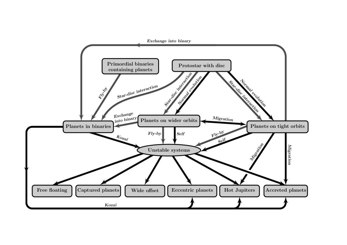
Figure 15: Overview of the evolution of planetary systems. Grey arrows identify interactions with other stars, most of which occur in young stellar clusters. Examples of such are fly-bys and exchange encounters involving binary systems. Planetary systems similar to our own solar system belong to the box labelled “Planets on wider orbits”.

10.6 Observational signatures of fly-bys

As shown in this paper, the principal effect of fly-bys is that they may trigger planet-planet scattering in otherwise stable planetary systems. However, the post-scattering systems cannot easily be distinguished from systems in which the scattering was triggered because the systems were intrinsically unstable (e.g. Moorhead & Adams, 2008; Jurić & Tremaine, 2008; Chatterjee et al., 2008).

One important aspect of fly-bys is, however, that only a fraction of stars suffer fly-bys. Hence, a large fraction of stars are singletons, and any planetary systems around them have not been perturbed by other stars. Hence, we predict that once planets can be detected in the semi-major axes region between 5 and 30 au around other stars many systems with similar properties to the solar system should be observed, if most systems start out with similar properties to the solar system.

Furthermore, as stellar encounters occur throughout the entire life-times of stellar clusters, we would expect that the fraction of planetary systems which are perturbed increase with cluster age. Hence, the properties of the population of planets in stellar clusters will depend on the age of the cluster.

Another important observational signature of planet-planet scattering, whether it is triggered by interactions with other stars or not, is, as is described both in this paper and in Scharf & Menou (2009); Veras et al. (2009), that it will produce planets on very wide orbits. Such planets must be observed in future imaging surveys, if planet-planet scattering is responsible for the observed eccentricities among extrasolar planets.

11 Summary

We have numerically simulated fly-bys involving planetary systems resembling our own solar system. Our motivation was to understand how a population of planetary systems evolve in stellar clusters, the birth environment of a large fraction of all stars. We have combined the fly-by simulations with our previous simulations of young stellar clusters, to calculate the effect on the population of planetary systems in the field today. The main results of the paper are:

1. Close fly-bys can lead to the immediate ejection of one or more planets from the host system. Such planets are either left unbound (ionisation), or are captured by the intruder star (exchange). Captured planets are often left on wide and moderately eccentric orbits, leaving them detectable in imaging surveys. Planets which remain bound to the host star after a close fly-by are most often on significantly more eccentric orbits. In a moderately-sized stellar cluster ($N=700$ stars, $r_{\rm h}=0.38$ pc) about 3 per cent of solar-system-like planetary systems will be involved in fly-bys leading to ionisation and/or capture of planets.

2. Wider fly-bys, which do not immediately remove planets from the host star, may still cause the ejection of planets on longer time scales by planet-planet scattering. The time between the fly-by and the onset of planet-planet scattering can be very long. For the four gas giants of the solar system we find that we can accurately predict if the system will suffer planet-planet scattering within $10^{8}$ years after a fly-by (e.g. Table 1), while the same is not easily done for the system where the masses of the planets have all been set to that of the planet Jupiter (4J) (e.g. Table 3). Planet-planet scattering significantly increases the fraction of planetary systems from which planets are ejected due to fly-bys. In, for example, the case of the 4G planetary systems and encounters with $r_{\rm min}<100$ au and $m_{\rm I}=0.6M_{\odot}$ the fraction of systems which suffer ejections is increased by a factor of three from the time of the fly-by until $10^{8}$ years later.

3. If the intruder in a fly-by is a very low-mass star or a brown dwarf, a sufficiently close fly-by may leave the intruder bound to the host star, potentially leading to drastic changes in the orbital properties of the planets orbiting the star. This can significantly increase the effect that such fly-bys have on planetary systems compared to what we would naively expect; for stellar mass intruders the magnitude of the change in the planetary orbits due to the fly-by decreases with decreasing intruder-star mass, suggesting that sub-stellar mass intruders would do very little damage to planetary systems. We have performed a large number of scattering experiments between a single-planet system and low-mass intruders to measure the rate at which the intruder may become bound to the host star. We find that, depending on the velocity dispersion of the cluster, and given the log-normal IMF of Chabrier (2001, 2002), up to few per cent of solar-system-like planetary systems may be involved in fly-bys that result in the capture of the low-mass intruder. Of course, if real clusters have an even larger number of low-mass intruders than suggested by Chabrier (2001, 2002), the fraction of systems involved in encounters with such objects will increase.

4. Fly-bys in general excite the eccentricities of planets left bound to either the host or the intruder star, both through direct scattering off the intruder, and through any subsequent planet-planet scattering. We find that the eccentricity distribution of planets which have been scattered inwards due to fly-bys in the 4G system is similar to that of the observed extrasolar planets (see Fig. 7 and discussion in section 9.2). Planetary systems where the masses are more similar (e.g. GM & 4J) tend to overproduce eccentric planets compared to the observed extrasolar planets.

5. Planet-planet scattering, triggered either by fly-bys or by primordial instability decreases the semi-major axes of one or more planets while leaving others on either much wider orbits, or unbinds them entirely. In our simulations of the four gas giants, we find that planets are only rarely scattered onto orbits tighter than 4 au, which is not consistent with the semi-major axes of observed planets. To reproduce the extrasolar planet population it is thus needed to allow for disc migration before the fly-by, allowing for planets to be on orbits inside the ice-line.

6. During the phase of planet-planet scattering, one or more planets are successively scattered onto wider and wider orbits until they become unbound. Such planets can, since they are so far from the host star, be observed using imaging techniques.

While not studied in this paper (but see Malmberg et al., 2007; Malmberg & Davies, 2009) another important type of encounters is binary-single encounters, in which a single star encounters a stellar binary system. Such encounters can, depending on the masses of the stars, leave the initially single star in the binary, replacing one of the original binary components. The key point here is that in such binaries, any planetary system will be randomly oriented with respect to the stellar companion, and as such will often be highly inclined with respect to the latter. In highly inclined binaries ($i>39.2^{\circ}$) the Kozai mechanism operates, exciting the eccentricities of the planets and thereby potentially triggering planet-planet scattering.

We have combined our results of how fly-bys affect planetary systems with the rate at which encounters in young stellar clusters occur, to measure how important such encounters are. As an example, we can look at the effects of fly-bys on the four gas giants of the solar system. We find that in between 5 and 15 per cent of such systems, fly-bys will trigger planet-planet scattering, leading to the ejection of one or more planets. The fraction of systems from which planets are ejected varies slowly with the number of stars in the cluster, $N$. More stars are believed to form in low-$N$ clusters than in more rich clusters. Hence, the contribution from rather small clusters to the field population of planetary systems that have been made unstable by fly-bys, can be significant. An important point regarding the fraction of systems that are affected by fly-bys concerns the properties of the systems before any stellar encounters. To explain the observed semi-major axes distribution many systems must initially have contained gas giants on much tighter orbits than what is seen in the solar system. The effects of fly-bys on such systems have not yet been explored, but will be the topic of a forthcoming paper.

In summary, fly-bys in young clusters will significantly change the properties of the population of planetary systems which initially resemble the solar system.

Appendix A Analytical formulae predicting the effects of fly-by’s

In order to write down the equations we use the standard Keplerian orbital elements describing the shape of the orbits, as well as the orientation of the intruder star’s orbit with respect to the orbit of the planet.

Let, $a_{\rm p}$ be the semi-major axis and $e_{\rm p}$ the eccentricity of the planet long before the encounter while $e_{\rm I}$ is the eccentricity of the intruder star in its hyperbolic orbit around the barycentre of the planetary system.

In order to define the orientation angles we define the line of nodes as the line formed by the intersection of the orbital planes of the planet and the intruder star. The ascending node is the point on this line at which the intruder star cross the orbital plane of the planet, measured in the orbital plane of the planet in the the same direction as the angular momentum vector of the planetary system. The longitude of the ascending node, $\Omega$ is measured from the pericentre of the planet in its orbital plane. Furthermore, $i$ is the inclination between the two orbital planes and $\omega$ is the longitude of pericentre of the intruder star, measured in its orbital plane from the ascending node, in the direction of its motion around the planetary system.

Finally, we define $m_{\rm H}$ to be the mass of the host star, $m_{\rm p}$ to be the mass of the planet, $m_{\rm I}$ to be the mass of the intruder star and $r_{\rm min}$ to be the minimum separation between the stars in the fly-by. We write the sum of the mass of the planetary system (planet and host star) as $M_{\rm ps}$ and the sum of the mass of the planetary system and the intruder star as $M_{\rm tot}$.

For planets on initially eccentric orbits the change in eccentricity, $\delta e$ is (Heggie & Rasio, 1996):

$$\delta e=-\frac{15}{4}\frac{m_{\rm I}}{\sqrt{M_{\rm ps}M_{\rm tot}}}\left(\frac{a_{\rm p}}{r_{\rm min}}\right)^{3/2}\frac{e_{\rm p}\sqrt{1-e_{\rm p}^{2}}}{(1+e_{\rm I})^{3/2}}\\ \times\left\{\sin^{2}{i}\sin{2\Omega}\left[\arccos(-1/e_{\rm I})+\sqrt{e_{\rm I}^{2}-1}\right]+\right.\\ \left.\quad\quad{}\frac{1}{3}\left[(1+\cos^{2}{i})\cos{2\omega}\sin{2\Omega}+\right.\right.\\ \left.\left.\quad\quad{}2\cos{i}\sin{2\omega}\cos{2\Omega}\right]\frac{(e_{\rm I}^{2}-1)^{3/2}}{e_{\rm I}^{2}}\right\}.$$ (20)

This result vanish if the eccentricity of the planet equals zero, which is why one must include higher order terms in the derivation. For a distant encounter the change in eccentricity for a planet on an initially circular orbit is (Heggie & Rasio, 1996):

$$\delta e=\frac{15}{8}\frac{m_{\rm I}\left|m_{\rm H}-m_{\rm p}\right|}{M^{2}_{ps}}\left(\frac{M_{\rm ps}}{M_{\rm tot}}\right)^{1/2}\left(\frac{a_{\rm p}}{r_{\rm min}}\right)^{5/2}\\ \frac{1}{e_{I}^{3}(1+e_{\rm I})^{5/2}}\times\left\{\cos^{2}{i}\sin^{2}{\omega}\left[f_{1}(e_{\rm I})(1-\frac{15}{4}\sin^{2}{i})\right.\right.\\ \left.\left.\quad\quad{}+\frac{2}{15}(e_{\rm I}^{2}-1)^{5/2}(1-5\sin^{2}{\omega}\sin^{2}{i})\right]^{2}\right.\\ \left.\quad\quad{}+\cos^{2}{\omega}\left[f_{1}(e_{\rm I})(1-\frac{5}{4}\sin^{2}{i})\right.\right.\\ \left.\left.\quad\quad{}+\frac{2}{15}(e_{\rm I}^{2}-1)^{5/2}(1-5\sin^{2}{\omega}\sin^{2}{i})\right]^{2}\right\}^{1/2},$$ (21)

where

$$f_{1}({e_{\rm I}})=e_{\rm I}^{4}\arccos(-1/e_{\rm I})+\frac{\sqrt{e_{\rm I}^{2}-1}}{15}(-2+9e_{\rm I}^{2}+8e_{\rm I}^{4})$$ (22)

Finally, for tight encounters involving planets on initially circular orbits, the change in eccentricity is (Heggie & Rasio, 1996):

$$\delta e=3\sqrt{2\pi}\frac{m_{\rm I}M_{\rm ps}^{1/4}}{M_{\rm tot}^{5/4}}\left(\frac{r_{\rm min}}{a_{\rm p}}\right)^{3/4}\frac{(e_{\rm I}+1)^{3/4}}{e_{\rm I}^{2}}\\ \times\exp\left[-\left(\frac{M_{\rm ps}}{M_{\rm tot}}\right)^{1/2}\left(\frac{r_{\rm min}}{a}\right)^{3/2}\frac{\sqrt{e_{\rm I}^{2}-1}-\arccos{(1/e_{\rm I})}}{(e_{\rm I}-1)^{3/2}}\right]\\ \times\cos^{2}{\frac{i}{2}}\left[\cos^{4}{\frac{i}{2}}+\frac{4}{9}\sin^{4}{\frac{i}{2}}\right.\\ \left.\quad\quad{}+\frac{4}{3}\cos^{2}{\frac{i}{2}}\sin^{2}{\frac{i}{2}}\cos{(4\omega+2\Omega)}\right]^{1/2}.$$ (23)

In fly-bys involving planetary systems containing multiple planets, not only the change in eccentricity, $e$, but also the change in inclination, $i$, is important. Thus, we have, using the same approach as in Heggie & Rasio (1996), derived an equation for the change in inclination of the planet, $\delta i_{\rm p}$, with respect to the plane of its original orbit:

$$\sin{(\delta i_{\rm p})}=\frac{3\pi m_{\rm I}}{8}\sqrt{\frac{2}{M_{\rm tot}M_{\rm ps}(1-e_{\rm p}^{2})}}\left(\frac{a_{\rm p}}{r_{\rm min}}\right)^{3/2}\\ \times\sin{i}\cos{i}\left[(1+3e_{\rm p}^{2})^{2}\sin^{2}{\Omega}+(1-e_{\rm p}^{2})^{2}\cos^{2}{\Omega}\right]^{1/2}$$ (24)

This expression is for a fly-by with the intruder on a parabolic orbit and has been averaged over the argument of pericentre ($\omega$).

References

- Aarseth (2003) Aarseth S. J., 2003, Gravitational N-Body Simulations. Gravitational N-Body Simulations, by Sverre J. Aarseth, pp. 430. ISBN 0521432723. Cambridge, UK: Cambridge University Press, November 2003.
- Adams (2010) Adams F. C., 2010, ArXiv e-prints
- Adams et al. (2004) Adams F. C., Hollenbach D., Laughlin G., Gorti U., 2004, ApJ, 611, 360
- Adams & Laughlin (2001) Adams F. C., Laughlin G., 2001, Icarus, 150, 151
- Adams & Myers (2001) Adams F. C., Myers P. C., 2001, ApJ, 553, 744
- Adams et al. (2006) Adams F. C., Proszkow E. M., Fatuzzo M., Myers P. C., 2006, ApJ, 641, 504
- Armitage (2000) Armitage P. J., 2000, A&A, 362, 968
- Barbieri et al. (2002) Barbieri M., Marzari F., Scholl H., 2002, A&A, 396, 219
- Barnes & Quinn (2004) Barnes R., Quinn T., 2004, ApJ, 611, 494
- Battinelli & Capuzzo-Dolcetta (1991) Battinelli P., Capuzzo-Dolcetta R., 1991, MNRAS, 249, 76
- Boss (1997) Boss A. P., 1997, Science, 276, 1836
- Chabrier (2001) Chabrier G., 2001, ApJ, 554, 1274
- Chabrier (2002) Chabrier G., 2002, ApJ, 567, 304
- Chambers (1999) Chambers J. E., 1999, MNRAS, 304, 793
- Chatterjee et al. (2008) Chatterjee S., Ford E. B., Matsumura S., Rasio F. A., 2008, ApJ, 686, 580
- Cumming et al. (2008) Cumming A., Butler R. P., Marcy G. W., Vogt S. S., Wright J. T., Fischer D. A., 2008, PASP, 120, 531
- Duquennoy & Mayor (1991) Duquennoy A., Mayor M., 1991, A&A, 248, 485
- Elmegreen & Clemens (1985) Elmegreen B. G., Clemens C., 1985, ApJ, 294, 523
- Fabrycky & Tremaine (2007) Fabrycky D., Tremaine S., 2007, ApJ, 669, 1298
- Fabrycky & Murray-Clay (2010) Fabrycky D. C., Murray-Clay R. A., 2010, ApJ, 710, 1408
- Ford & Rasio (2008) Ford E. B., Rasio F. A., 2008, ApJ, 686, 621
- Forgan & Rice (2009) Forgan D., Rice K., 2009, MNRAS, 400, 2022
- Fragner & Nelson (2009) Fragner M. M., Nelson R. P., 2009, A&A, 505, 873
- Fregeau et al. (2006) Fregeau J. M., Chatterjee S., Rasio F. A., 2006, ApJ, 640, 1086
- Heggie & Hut (2003) Heggie D., Hut P., 2003, The Gravitational Million-Body Problem: A Multidisciplinary Approach to Star Cluster Dynamics. Cambridge University Press, 2003, 372 pp.
- Heggie (1975) Heggie D. C., 1975, MNRAS, 173, 729
- Heggie & Rasio (1996) Heggie D. C., Rasio F. A., 1996, MNRAS, 282, 1064
- Heinze et al. (2010) Heinze A. N., Hinz P. M., Sivanandam S., Kenworthy M., Meyer M., Miller D., 2010, ApJ, 714, 1551
- Hills (1984) Hills J. G., 1984, AJ, 89, 1559
- Hurley & Shara (2002) Hurley J. R., Shara M. M., 2002, ApJ, 565, 1251
- Hut et al. (1992) Hut P., McMillan S., Romani R. W., 1992, ApJ, 389, 527
- Jurić & Tremaine (2008) Jurić M., Tremaine S., 2008, ApJ, 686, 603
- Kalas et al. (2008) Kalas P., Graham J. R., Chiang E., Fitzgerald M. P., Clampin M., Kite E. S., Stapelfeldt K., Marois C., Krist J., 2008, Science, 322, 1345
- Kobayashi & Ida (2001) Kobayashi H., Ida S., 2001, Icarus, 153, 416
- Kozai (1962) Kozai Y., 1962, AJ, 67, 591
- Kroupa et al. (1993) Kroupa P., Tout C. A., Gilmore G., 1993, MNRAS, 262, 545
- Laskar (2000) Laskar J., 2000, Physical Review Letters, 84, 3240
- Levison et al. (1998) Levison H. F., Lissauer J. J., Duncan M. J., 1998, AJ, 116, 1998
- Malmberg & Davies (2009) Malmberg D., Davies M. B., 2009, MNRAS, 394, L26
- Malmberg et al. (2007) Malmberg D., Davies M. B., Chambers J. E., 2007, MNRAS, 377, L1
- Malmberg et al. (2007) Malmberg D., de Angeli F., Davies M. B., Church R. P., Mackey D., Wilkinson M. I., 2007, MNRAS, 378, 1207
- Marois et al. (2008) Marois C., Macintosh B., Barman T., Zuckerman B., Song I., Patience J., Lafrenière D., Doyon R., 2008, Science, 322, 1348
- Matsumura et al. (2010) Matsumura S., Thommes E. W., Chatterjee S., Rasio F. A., 2010, ApJ, 714, 194
- Mayor & Queloz (1995) Mayor M., Queloz D., 1995, Nature, 378, 355
- Moorhead & Adams (2008) Moorhead A. V., Adams F. C., 2008, Icarus, 193, 475
- Nagasawa et al. (2008) Nagasawa M., Ida S., Bessho T., 2008, ApJ, 678, 498
- Parker & Goodwin (2009) Parker R. J., Goodwin S. P., 2009, MNRAS, 397, 1041
- Plummer (1911) Plummer H. C., 1911, MNRAS, 71, 460
- Pollack et al. (1996) Pollack J. B., Hubickyj O., Bodenheimer P., Lissauer J. J., Podolak M., Greenzweig Y., 1996, Icarus, 124, 62
- Portegies Zwart et al. (2001) Portegies Zwart S. F., McMillan S. L. W., Hut P., Makino J., 2001, MNRAS, 321, 199
- Rasio & Ford (1996) Rasio F. A., Ford E. B., 1996, Science, 274, 954
- Raymond et al. (2009) Raymond S. N., Barnes R., Veras D., Armitage P. J., Gorelick N., Greenberg R., 2009, ApJ, 696, L98
- Scharf & Menou (2009) Scharf C., Menou K., 2009, ApJ, 693, L113
- Scholz et al. (2009) Scholz A., Geers V., Jayawardhana R., Fissel L., Lee E., Lafreniere D., Tamura M., 2009, ApJ, 702, 805
- Spurzem et al. (2009) Spurzem R., Giersz M., Heggie D. C., Lin D. N. C., 2009, ApJ, 697, 458
- Thébault et al. (2006) Thébault P., Marzari F., Scholl H., 2006, Icarus, 183, 193
- Thébault et al. (2004) Thébault P., Marzari F., Scholl H., Turrini D., Barbieri M., 2004, A&A, 427, 1097
- Triaud & et al. (2010) Triaud A. H. M. J., et al. 2010, A&A, submitted
- van den Bergh (1981) van den Bergh S., 1981, PASP, 93, 712
- Veras et al. (2009) Veras D., Crepp J. R., Ford E. B., 2009, ApJ, 696, 1600
- Zakamska & Tremaine (2004) Zakamska N. L., Tremaine S., 2004, AJ, 128, 869