Tunable backaction of a dc SQUID on an integrated micromechanical resonator

Abstract

We have measured the backaction of a dc superconducting quantum interference device (SQUID) position detector on an integrated 1 MHz flexural resonator. The frequency and quality factor of the micromechanical resonator can be tuned with bias current and applied magnetic flux. The backaction is caused by the Lorentz force due to the change in circulating current when the resonator displaces. The experimental features are reproduced by numerical calculations using the resistively and capacitively shunted junction (RCSJ) model.

It has recently been demonstrated that a macroscopic mechanical resonator can be put in a quantum state O’Connell et al. (2010) by coupling it to another quantum system. At the same time, linear detectors coupled to mechanical resonators are rapidly approaching the quantum limit on position detection. This limit implies that the resonator position cannot be measured with arbitrary accuracy, as the detector itself affects the resonator position Caves et al. (1980). This is an example of backaction. Backaction does not just impose limits, it can also work to one’s advantage: Backaction can cool the resonator, squeeze its motion, and couple and synchronize multiple resonators. Different backaction mechanisms have been identified: When using optical interferometers Gigan et al. (2006); Arcizet et al. (2006); Thompson et al. (2008); Anetsberger et al. (2009) or electronic resonant circuits Teufel et al. (2008); Brown et al. (2007); Rocheleau et al. (2010), backaction results from radiation pressure. In single-electron transistors (SET) Naik et al. (2006), Cooper-pair boxes LaHaye et al. (2009), carbon nanotube quantum dots Steele et al. (2009); Lassagne et al. (2009), or atomic and quantum point contacts Flowers-Jacobs et al. (2007); Stettenheim et al. (2010) backaction is due to the tunneling of electrons. Recently, we have used a dc SQUID as a sensitive detector of the position of an integrated mechanical resonator Etaki et al. (2008). This embedded resonator-SQUID geometry enables the experimental realization of a growing number of theoretical proposals for which a good understanding of the backaction is required Zhou and Mizel (2006); Blencowe and Buks (2007); Xue et al. (2007a); Huo and Long (2008); Nation et al. (2008); Buks and Blencowe (2006); Xue et al. (2007b).

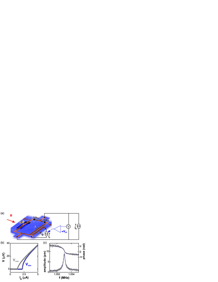
Figure 1: (a) Schematic overview of the dc SQUID with the suspended beam and measurement setup. A magnetic field $B$ transduces a beam displacement $u$ into a change in magnetic flux. A bias current $I_{B}$ is sent through the SQUID and its output voltage is measured. The flux $\Phi$ is fine-tuned with a stripline current $I_{F}$ that is controlled by a feedback circuit (dashed) that keeps the output voltage $V$ at $V_{SP}$. (b) The bias current dependence of the measured $V_{\mathrm{min}}$ and $V_{\mathrm{max}}$. (c) The amplitude (bottom) and phase (top) response. The line is a fitted harmonic oscillator response cro .

In this Letter, we present experiments that show that the dc SQUID detector exerts backaction on the resonator. By adjusting the bias conditions of the dc SQUID the frequency and damping of the mechanical resonator change. The backaction by the dc SQUID has a different origin than in the experiments mentioned above: It is due to the Lorentz force generated by the circulating current. Numerical calculations using the RCSJ model for the dc SQUID Clarke and Braginski (2004) reproduce the experimental features.

The device (Fig. 1a) consists of a dc SQUID with proximity-effect-based junctions Etaki et al. (2008). A part of one arm is underetched, forming a $1~{}\mathrm{MHz}$ flexural resonator with length $\ell=50~{}\mathrm{\mu m}$. In this Letter we present data on a device in an in-plane magnetic field of $B=100~{}\mathrm{mT}$. Measurements have been performed at several magnetic fields and on an additional device; the observed backaction is similar sup . First the dc SQUID is characterized. The output voltage of a dc SQUID depends on the magnetic flux through its loop $\Phi$ Clarke and Braginski (2004) and we measure the minimum and maximum voltage ($V_{\mathrm{min}}$ and $V_{\mathrm{\max}}$) by sweeping the flux over a few flux quanta $\Phi_{0}=h/2e$ with a nearby stripline (Fig. 1a). This is repeated for different bias currents to obtain the current-voltage curves shown in Fig. 1b. The maximum critical current is $I_{c}^{\mathrm{max}}=2.19~{}\mathrm{\mu A}$ and the normal-state resistance of the junctions is $R=15.6~{}\mathrm{\Omega}$. After this characterization, the dc SQUID is operated at a given setpoint voltage $V_{SP}$ using a feedback loop that adjusts the flux via the stripline current Etaki et al. (2008); Clarke and Braginski (2004). The feedback loop is used to reduce low-frequency flux noise and flux drift and has a bandwidth of $\sim 2~{}\mathrm{kHz}$, i.e., it does not respond to the $1~{}\mathrm{MHz}$ resonator signal.

The fundamental mode of the flexural resonator is excited using a piezo element underneath the sample and the displacement of the beam is detected as follows: The in-plane magnetic field transduces a displacement of the beam $u$ into a flux change $\sim\ell Bu$, which in turn changes the voltage over the dc SQUID. This voltage is amplified using a cryogenic high-electron mobility transistor followed by a room temperature amplifier and then recorded using a network analyzer. Figure 1c shows the amplitude and phase of the measured response, from which the resonance frequency $f_{R}$ and quality factor $Q$ are obtained.

To observe backaction of the dc SQUID detector on the resonator, the frequency response is measured for different bias conditions of the SQUID. Figure 2 shows that both $f_{R}$ and $Q$ depend on the bias current $I_{B}$. The resonance frequency saturates at $f_{0}=1.053010~{}\mathrm{MHz}$ for large positive and negative bias currents. However, when decreasing the $I_{B}$, $f_{R}$ first goes up by a few hundred Hz around $I_{c}^{\mathrm{max}}$ and then it decreases rapidly with about -2000 Hz at the lowest stable setpoint voltage. This is more than $10\times$ the linewidth $f_{R}/Q=194~{}\mathrm{Hz}$ of the resonance shown in Fig. 1c. Figure 2b shows that the quality factor of the resonator changes from $Q_{0}=5300$ to less than 2000. Similar to the resonance frequency, first an increase and then a stronger decrease in $Q$ is observed when lowering the bias current.

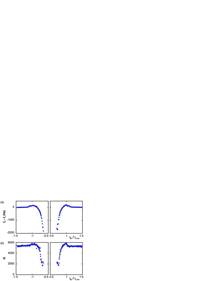
Figure 2: Frequency shift (a) and quality factor (b) plotted versus the normalized bias current. The voltage setpoint was halfway between $V_{\mathrm{min}}$ and $V_{\mathrm{max}}$ in these measurements.

Figure 3 shows that the frequency and damping can also be changed by adjusting $V_{SP}$, i.e., the flux through the SQUID loop. The shifts are largest for low setpoints and low bias currents (dark regions). The regions with a lower frequency coincide with the regions where the damping has increased. Bias points with positive frequency shifts and increases in $Q$ are indicated in white. Finally, by varying the driving power we confirm that the observed effects are not due to nonlinearities in the SQUID or in the resonator sup .

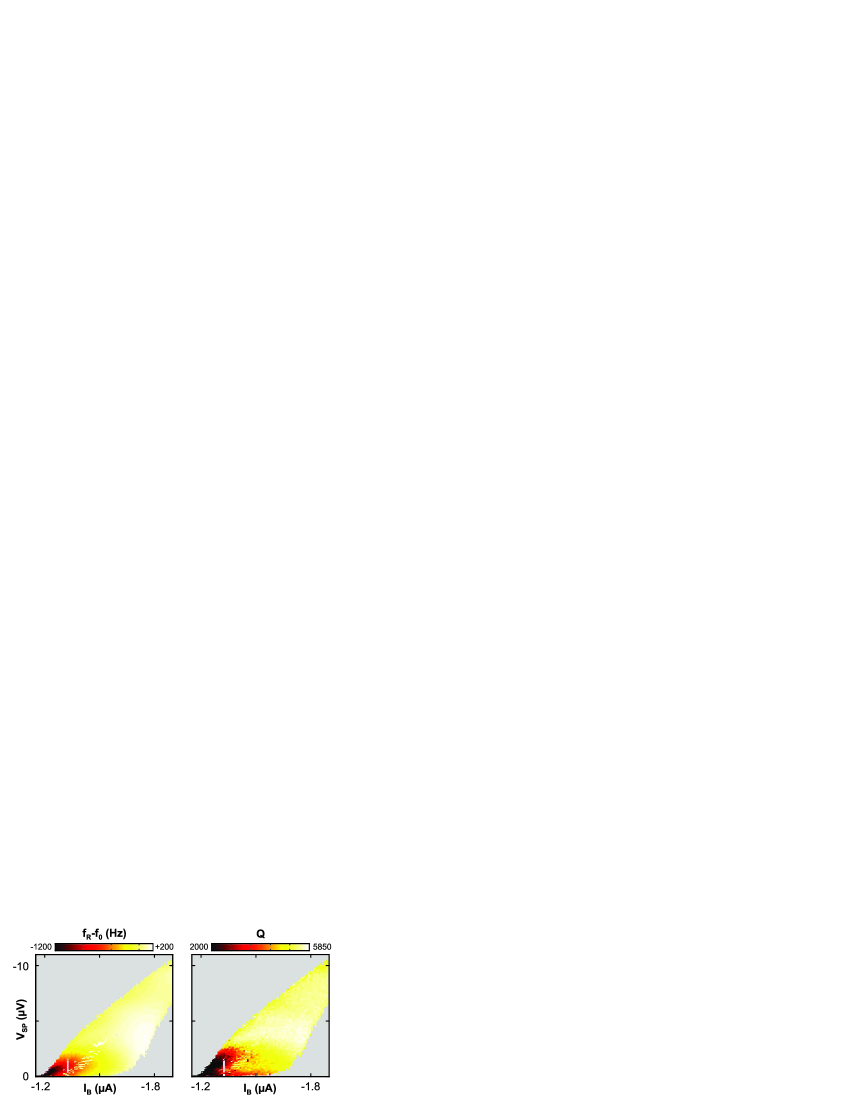
Figure 3: Measured bias current and voltage setpoint dependence of the frequency shift (left) and damping (right). Points without a good lock are indicated in gray.

Unlike for position detectors such as the SET where the backaction originates from the Coulomb force, the backward coupling between the SQUID and the beam is the Lorentz force $F_{L}$ Blencowe and Buks (2007); Nation et al. (2008). This force is due to the current that flows through the beam in the presence of the magnetic field that couples the resonator and the SQUID. A displacement changes the flux, and this in turn changes the circulating current in the loop $J$ Clarke and Braginski (2004), giving a different force on the beam. In addition, resonator motion yields a time-varying flux through the loop, which induces an electro-motive force and thereby also generates currents that change the Lorentz force Cleland and Roukes (1999).

The displacement of the fundamental out-of-plane flexural mode $u$ is given by Cleland and Roukes (2002):

$$m\ddot{u}+m\omega_{0}\dot{u}/Q_{0}+m\omega_{0}^{2}u=F_{d}(t)+F_{L}(t).$$ (1)

The resonator has a mass $m$, (intrinsic) frequency $f_{0}=\omega_{0}/2\pi$ and quality factor $Q_{0}$. $F_{d}$ is the driving force and $F_{L}=aB\ell(I_{B}/2+J)$ is the Lorentz force. Here, $a=(u\ell)^{-1}\int_{0}^{\ell}u(x)~{}\mathrm{d}x\approx 0.9$ for the fundamental mode, so that also $\partial\Phi/\partial u=aB\ell$ Etaki et al. (2008); Cleland and Roukes (2002). For small amplitudes and low resonator frequencies (much smaller than the characteristic SQUID frequency $\omega_{c}=\pi RI_{c}^{\mathrm{max}}/\Phi_{0}$), the average circulating current can be expanded in the displacement and velocity $\dot{u}$ sup :

$$J(u,\dot{u})=J_{0}+\frac{\partial J}{\partial\Phi}aB\ell u+\frac{\partial J}{\partial\dot{\Phi}}aB\ell\dot{u}.$$ (2)

Inserting Eq. (2) into Eq. (1) shows that the $\partial J/\partial\Phi$ term affects the spring constant $m\omega_{R}^{2}$ and thus $f_{R}$, whereas the $\partial J/\partial{\dot{\Phi}}$ term renormalizes the damping. The shifted resonance frequency and quality factor are:

$$f_{R} = f_{0}\left(1-\Delta_{f}\jmath_{\phi}\right)^{1/2},\textrm{~{}with~{}}\Delta_{f}=\frac{a^{2}B^{2}\ell^{2}}{m\omega_{0}^{2}}\frac{I_{c}^{\mathrm{max}}}{2\Phi_{0}},$$ (3)

$$Q = Q_{0}\frac{f_{R}}{f_{0}}\frac{1}{1-\Delta_{Q}\jmath_{\dot{\phi}}},\textrm{~{}with~{}}\Delta_{Q}=\frac{a^{2}B^{2}\ell^{2}}{m\omega_{0}R}\frac{Q_{0}}{2\pi}.$$ (4)

Here, $\jmath_{\phi}=\partial J/\partial\Phi\times 2\Phi_{0}/I_{c}^{\mathrm{max}}$ and $\jmath_{\dot{\phi}}=\partial J/\partial\dot{\Phi}\times 2\omega_{c}\Phi_{0}/I_{c}^{\mathrm{max}}$ are the scaled flux-to-current transfer functions Hilbert and Clarke (1985). The former indicates how much the circulating current changes when the flux through the ring is altered, whereas the latter quantifies the effect of a time-dependent flux on the circulating current. These functions were first studied in the analysis of the dynamic input impedance of tuned SQUID amplifiers Hilbert and Clarke (1985); Falferi et al. (1997) and are intrinsic properties of the SQUID.

Before looking in more detail at the transfer functions, we first focus on the coupling. The dimensionless parameters $\Delta_{f}$ Huo and Long (2008) and $\Delta_{Q}$ characterize the backaction strength. They contain the term $aB\ell$ squared as both the flux change and the Lorentz force are proportional to the magnetic field. This implies that the backaction remains the same when the direction of the magnetic field is reversed and this is what we observe experimentally. $\Delta_{f}$ is proportional to $I_{c}^{\mathrm{max}}$, whereas the damping induced by the SQUID depends on $R$. By a careful design of the resonator and SQUID, the backaction strengths can be tuned over a wide range. Eqs. (3) and (4) show that the largest backaction occurs for large flux changes $aB\ell$, low spring constants $m\omega^{2}_{0}$, and large circulating currents, i.e., large $I_{0}$ and low $R$. For the device studied in this Letter, we estimate $\Delta_{f}=4.1\times 10^{-4}$ and $\Delta_{Q}=2.8\times 10^{-4}$. Finally, note that the two coupling parameters are related by $\Delta_{Q}=\Delta_{f}\times Q_{0}\omega_{0}/\omega_{c}$.

So far, the analysis did not assume anything about the number of junctions, nor about their microscopic details. To obtain the transfer functions $\jmath_{\phi}$ and $\jmath_{\dot{\phi}}$, we model the junctions in the dc SQUID using the RCSJ model Clarke and Braginski (2004). The transfer functions can be calculated analytically in certain limits cal . However, to obtain their full bias-condition dependence, $\jmath_{\phi}$ and $\jmath_{\dot{\phi}}$ must be calculated numerically. This is done by simulating the dynamics of the SQUID in the presence of a time-varying flux sup . Figure 4a shows the bias-dependence of $\jmath_{\phi}$. In the region where $V=0$, the circulating current redistributes the bias current between the two junctions such that no voltage develops. Here the circulating current is of the order of $I_{c}^{\mathrm{max}}/2$, which gives $\jmath_{\phi}\sim-1$ (blue). In the dissipative region ($V\neq 0$), the circulating current is suppressed. Therefore, the circulating current changes rapidly close to the edge of the dissipative region. The orange color in Fig. 4a indicates that $\jmath_{\phi}$ is large and positive near the critical current. The largest downward frequency shift is expected near a half-integer number of flux quanta, whereas $\jmath_{\phi}$ vanishes for integer flux. With the value of the coupling parameter $\Delta_{f}$ and the resonance frequency $f_{0}$ the frequency shift is calculated as shown in Fig. 4c. The maximum value $\jmath_{\phi}=53$ gives a frequency shift of $-12~{}\mathrm{kHz}$ in the lower-left corner, which has to be compared with the experimental value of $\sim-2~{}\mathrm{kHz}$. Increasing the bias current above the critical current results in a smaller $\jmath_{\phi}$ (light yellow and light blue) that depends linearly on the inductive screening parameter $\beta_{L}$ Clarke and Braginski (2004) for the experimental conditions. In this region the simulations predict both positive (blue) and negative (yellow) value for $\jmath_{\phi}$. Positive and negative shifts are also observed in the experiment (Figs. 2 and 3). The largest negative value found in the simulations of that region is $\jmath_{\phi}=-0.65$, which results in an increase in $f_{R}$ of $\sim 140~{}\mathrm{Hz}$, which is in agreement with the observed value of $\sim 200~{}\mathrm{Hz}$ (Fig. 2a). For even larger bias currents, the frequency shift vanishes $f_{R}\approx f_{0}$. This corresponds to the flat regions in Fig. 2a.

The change in damping is determined by $\jmath_{\dot{\phi}}$ as indicated by Eq. (4). Its dependence on the bias conditions is shown in Fig. 4b. Well inside the experimentally inaccessible non-dissipative region $\jmath_{\dot{\phi}}\sim+1$ and the backaction results in a small increase in $Q$. In the opposite limit of large bias currents $\jmath_{\dot{\phi}}=-\pi$ (light blue). This value combined with the small value of $\Delta_{Q}$ implies that the quality factor in the flat region in Fig. 2b is close to the intrinsic Q-factor, $Q_{0}$. In this region the small additional damping is due to the current induced by the time-varying flux $\dot{\Phi}/2R$, which is dissipated in the junction resistances cal . This contribution is well-known from magnetomotive readout of mechanical resonators Cleland and Roukes (1999). When lowering the bias current, $\jmath_{\dot{\phi}}$ changes sign and rises to about $+500$. This reduces the damping and might even lead to instability ($Q<0$) if $\Delta_{Q}$ is large enough. This decrease of damping corresponds to the bumps in Fig. 2b. The largest observed quality factor $Q=5800$ corresponds to $\jmath_{\dot{\phi}}=+400$, which is in reasonable agreement with the simulations. Close to the critical current, $\jmath_{\dot{\phi}}$ goes to large negative values leading to an enhanced dissipation. Figure 4d shows that the calculated Q-factor is indeed lowest near the critical current. In summary, our model shows that although the coupling strength is small, the dynamics of the dc SQUID greatly enhances the backaction.

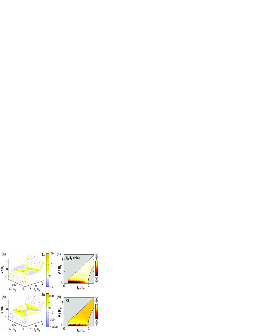
Figure 4: Surface plots with iso-voltage lines at different bias conditions of a dc SQUID. The (logarithmic) color-scale represents the calculated flux-to-current transfer functions $\jmath_{\phi}$ (a) and $\jmath_{\dot{\phi}}$ (b). With the values for $\Delta_{f}$ and $\Delta_{Q}$, the frequency shift (c) and quality factor change (d) are calculated. The simulation is done for the experimental conditions where the inductive screening parameter $\beta_{L}=0.21$ and the Stewart-McCumber parameter $\beta_{C}=0.23$ Clarke and Braginski (2004); sup .

Various interesting effects can be observed when the backaction is strong. If the resonator and SQUID are strongly coupled, the resonator temperature is set by the effective bath temperature Naik et al. (2006); Flowers-Jacobs et al. (2007) of the SQUID. The increased damping cools the resonator, but the shot noise in the bias current leads to an increase in the force noise on the resonator, heating it. The question whether the resonator temperature is above or below the environmental temperature should be addressed in future research. Furthermore, the dependence of $f_{R}$ and $Q$ on the bias conditions allows parametric excitation of the mechanical resonator by either modulating the flux or the bias current. This enables squeezing of the thermomechanical noise of the resonator Rugar and Grütter (1991); Huo and Long (2008). Finally, if the SQUID contains multiple, nearly identical mechanical resonators, these are coupled to each other by the backaction. This, in turn, can synchronize their motion and might lead to frequency entrainment if higher order terms in Eq. (2) become significant Shim et al. (2007). These examples are only a few intriguing possibilities of the rich physics connected to the backaction that we have described in this Letter.

Temperature and power dependence

Figures 5a and b show the temperature dependence of the resonance frequency and quality factor. These values are measured at large bias currents where the backaction is negligible. The frequency change due to temperature is small compared to the observed backaction (see main text). The intrinsic quality factor decreases significantly with increasing temperature. This rules out that the observed frequency shift and Q-factor change are caused by heating of the resonator due to Joule heating in the junctions: We observe an increase in quality factor with increasing bias current and voltage setpoint (i.e. dissipation), but a decrease in quality factor with increasing temperature. An increased damping at higher temperatures is seen more often in micro- or nanomechanical resonators Yamaguchi et al. (2004); Hüttel et al. (2009); LaHaye et al. (2004); Zolfagharkhani et al. (2005).

The observed frequency shift and change in damping do not depend on the driving power. As shown in Figure 5c, the measured resonator response stays the same in all panels. Although the driving power is changed by three orders of magnitude, the only effect is that the signal-to-noise ratio becomes better when increasing the power.

For the highest driving power ($P_{d}=-75~{}\mathrm{dBm}$) and highest Q-factor ($Q\sim 5800$) the amplitude of the resonator motion is $u_{\mathrm{max}}=20~{}\mathrm{pm}$, as determined using the calibrated displacement responsivity Etaki et al. (2008). The flux through the dc SQUID is then modulated with an amplitude $aB\ell u_{\mathrm{max}}=0.02~{}\mathrm{\Phi_{0}}$. So even for the largest resonator motion, the change in flux is much smaller than a flux quantum. Exactly on resonance, the piezo motion is $Q$ times smaller than $u_{\mathrm{max}}$, about $3~{}\mathrm{fm}$. The driving force $F_{d}$ is then given by the resonator mass $m$ times the acceleration of the piezo element, $F_{d}=m\omega^{2}u_{p}\approx m\omega_{0}^{2}u_{p}$. The measurements shown in the main text are done with a driving power of $-80~{}\mathrm{dBm}$ ($F_{d}=48\,\mathrm{fN}$).

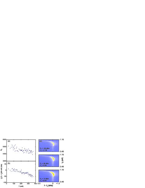
Figure 5: Temperature dependence of the intrinsic quality factor $Q_{0}$ (a) and resonator frequency $f_{0}$ (b). (c) Colorscale plot of the oscillator response at $B=100~{}\mathrm{mT}$ at different driving powers $P_{d}$. This measurement is done with a voltage setpoint halfway between $V_{\mathrm{min}}$ and $V_{\mathrm{max}}$.

Device B

All effects that we have observed in the device that we discuss in the main text have also been measured in a second device. The resonator in this dc SQUID operates around $2~{}\mathrm{MHz}$. The maximum critical current of device B is $I_{c}^{\mathrm{max}}=2I_{0}=2.4~{}\mathrm{\mu A}$ at $B=115~{}\mathrm{mT}$ and $I_{c}^{\mathrm{max}}=1.0~{}\mathrm{\mu A}$ at $B=130~{}\mathrm{mT}$.

In the measurements on device B, the feedback loop could not maintain the SQUID voltage for low voltage setpoints. Also, a less sensitive, room temperature amplifier was used for the resonator signal. Its lower gain resulted in an increased scatter in the data and the inability to explore the region with the highest backaction, i.e., at low bias current and low voltage setpoints. The measurements in Fig. 6 show qualitatively the same backaction as the data presented in the main text.

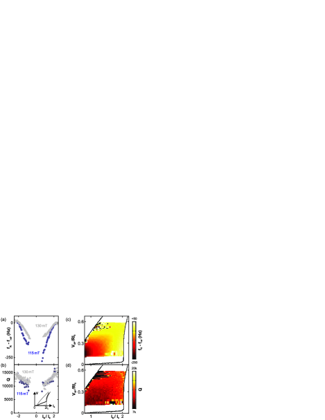
Figure 6: Backaction measurements of device B. (a) Frequency shift and (b) quality factor plotted versus the normalized bias current at $B=115\,\mathrm{mT}$ (circles) and $B=130\,\mathrm{m}T$ (triangles). The inset depicts the voltage setpoint for these measurements with respect to $V_{\mathrm{min}}$ and $V_{\mathrm{max}}$. Bias current and setpoint dependence of the frequency shift (c) and damping (d) at $B=115$ mT. The solid lines indicate the measured $V_{\mathrm{min}}$ and $V_{\mathrm{max}}$.

The RCSJ model for the dc SQUID

To calculate the backaction, the dc SQUID is modelled using the resistively- and capacitively-shunted junction (RCSJ) model. This widely-used model is discussed in detail in Ref. Clarke and Braginski (2004). The introduction to this model presented here is largely based on this review. A current $I_{B}$ is sent through the SQUID and the circulating current $J$ redistributes the current over the two junctions, which we assume to be identical. In the RCSJ model, the two junctions (labelled with $i=1,2$) are modelled as a resistor ($R$), capacitor ($C$) and an “ideal” Josephson junction with critical current $I_{0}$ in parallel. The voltage over each junction is related to the time derivative of the phase difference $\delta_{i}$ of the superconducting wave function: $V_{i}=\Phi_{0}\ \dot{\delta}_{i}/2\pi$, where $\Phi_{0}=h/2e=2.05\times 10^{-15}~{}\mathrm{Tm^{2}}$ is the flux quantum. Current conservation yields two second-order differential equations, governing the time-dependence of the phase differences $\delta_{1,2}$ of the junctions:

$$\frac{\Phi_{0}}{2\pi}C\ddot{\delta}_{1}+\frac{\Phi_{0}}{2\pi}\frac{1}{R}\dot{\delta}_{1}+I_{0}\sin\delta_{1} = \frac{1}{2}I_{B}+J,$$ (5)

$$\frac{\Phi_{0}}{2\pi}C\ddot{\delta}_{2}+\frac{\Phi_{0}}{2\pi}\frac{1}{R}\dot{\delta}_{2}+I_{0}\sin\delta_{2} = \frac{1}{2}I_{B}-J.$$ (6)

These equations are coupled to each other by the amount of flux piercing the loop:

$$\delta_{2}-\delta_{1}=2\pi\cdot\Phi_{\mathrm{tot}}/\Phi_{0}.$$ (7)

The total flux $\Phi_{\mathrm{tot}}$ has two contributions: the externally applied flux $\Phi$ (which also includes the flux due to the resonator displacement) and the flux due to the circulating current flowing through the inductance of the loop $L$, i.e., $\Phi_{\mathrm{tot}}=\Phi+LJ$.

The equations are scaled to simplify their numerical integration. This yields:

$$\beta_{C}\ddot{\delta_{1}}+\dot{\delta_{1}}+\sin\delta_{1} = \imath_{B}/2+\jmath$$ (8)

$$\beta_{C}\ddot{\delta_{2}}+\dot{\delta_{2}}+\sin\delta_{2} = \imath_{B}/2-\jmath$$ (9)

$$2\pi(\phi+\beta_{L}\jmath/2) = \delta_{2}-\delta_{1}.$$ (10)

The bias current and circulating current are normalized using the critical current: $\imath_{B}=I_{B}/I_{0}$ and $\jmath=J/I_{0}$. Furthermore, time is scaled using the characteristic frequency $\omega_{c}=2\pi RI_{0}/\Phi_{0}$, fluxes using the flux quantum, i.e., $\phi=\Phi/\Phi_{0}$, and voltages using the characteristic voltage $RI_{0}$ so that $v=V/RI_{0}=(\dot{\delta}_{1}+\dot{\delta}_{2})/2$. The parameter $\beta_{L}=2I_{0}L/\Phi_{0}$ and $\beta_{C}=2\pi I_{0}R^{2}C/\Phi_{0}$ are the inductive screening parameter and the Stewart-McCumber number respectively. The inductive screening parameter indicates how much a change in flux is screened by the circulating current $J$ flowing through the self-inductance of the loop $L$, whereas $\beta_{C}$ indicates the importance of inertial terms due to the junction capacitance $C$.

The three equations are integrated numerically for different bias conditions, i.e., different values for the bias current $I_{B}$ and for the flux $\Phi$ through the SQUID. Figure 7a shows typical examples of calculated time-traces of the circulating current $\jmath$ and voltage $v$. Both are rapidly oscillating at a frequency of $0.69~{}\omega_{c}$, which is the Josephson frequency that equals the average value of the voltage $\overline{v}$ Clarke and Braginski (2004). The maximum current that the dc SQUID can carry without generating a voltage equals the sum of the critical currents of the two junctions: $I_{c}^{\mathrm{max}}=2I_{0}$.

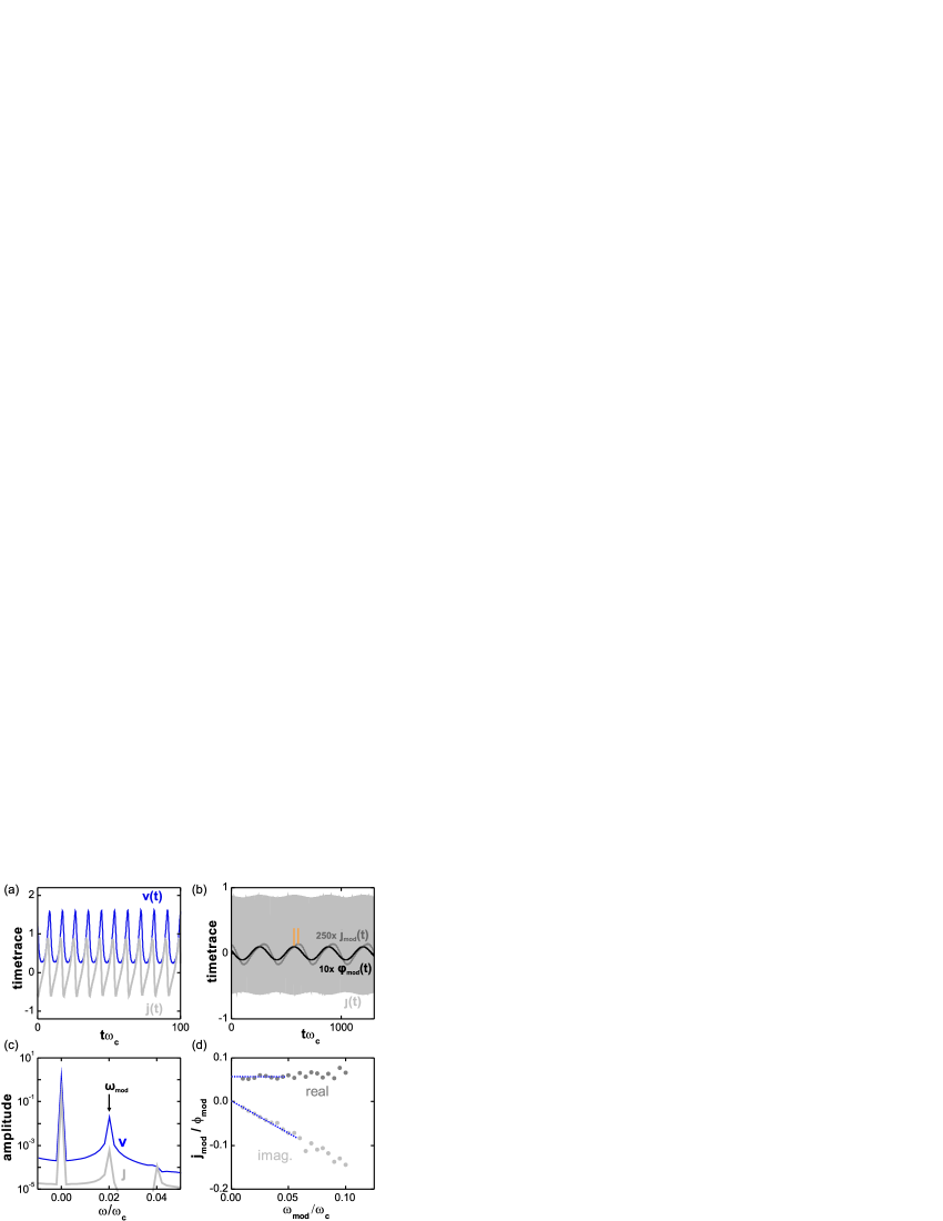
Figure 7: (a) Calculated timetrace of the circulating current $\jmath(t)$ and voltage $v(t)$ in the absence of noise. (b) Circulating current for a small ($\phi_{\mathrm{mod}}=0.01$) modulation of the flux with $\omega_{\mathrm{mod}}=0.02$. The time-averaged value of the circulating current $\overline{\jmath}(t)$ has a phase shift with respect to the modulation $\phi(t)$ as indicated by the orange lines. (c) Absolute value of the Fourier transform of the timetraces of the SQUID voltage and circulating current shown in (b). (d) The modulation frequency dependence of the real (dark gray) and imaginary (light gray) parts of the transfer function. The lines are a guide to the eye. These simulations were done for the dc SQUID parameters from the main text ($\beta_{L}=0.21$ and $\beta_{C}=0.23$) at $\imath_{B}=2$ and $\phi=0.25$.

The critical current ($I_{0}=1.1~{}\mathrm{\mu A}$) and the normal-state resistance ($R=15.6~{}\mathrm{\Omega}$) of the junctions are estimated from the IV-characteristics (Fig. 1b of the main text). Using finite-element simulations we estimate $L=175~{}\mathrm{pH}$ for our device. Finally, the capacitance $C=0.6~{}\mathrm{pF}$ is obtained from the position of the LC resonance in the dc SQUID Clarke and Braginski (2004).

Calculation of the transfer functions

When the resonator moves, the flux through the dc SQUID loop is altered, which in turn changes the average circulating current $J$. In principle, $J(t)$ could depend on the all the past displacements, $u(t^{\prime})$ for $t^{\prime}<t$. However, the dc SQUID reacts at a frequency ($\sim\omega_{c}/2\pi\sim 8\,\mathrm{GHz}$) that is much faster than that of the resonator ($1\,\mathrm{MHz}$), so the circulating current $J(t)$ is expected to depends on the instantaneous displacement $u(t)$. For small amplitudes ($u\ll\Phi_{0}/aB\ell$) the response is linear and gives a contribution $J_{1}(t)=c_{1}u(t)$. Another contribution comes from the velocity of the resonator, $\dot{u}$, which causes a time-varying flux. This generates an electromotive force in the SQUID loop (Faraday’s induction law), which also changes the circulating current by $J_{2}(t)=c_{2}\dot{u}(t)$. Combining these two effects gives $J(t)=J(u,\dot{u})=c_{1}u(t)+c_{2}\dot{u}(t)$. The values of the parameters $c_{1}$ and $c_{2}$ depend on the dynamics of the dc SQUID and are $c_{1}=\partial J/\partial u$ and $c_{2}=\partial J/\partial\dot{u}$. As discussed in the main text, these quantities are related to the intrinsic flux-to-current transfer functions, $\jmath_{\phi}=\Phi_{0}/(aB\ell I_{0})\times\partial J/\partial u$ and $\jmath_{\dot{\phi}}=\omega_{c}\Phi_{0}/(aB\ell I_{0})\times\partial J/\partial\dot{u}$.

In principle $\jmath_{\phi}$ can be obtained by calculating the average circulating current at different fluxes and then numerically differentiating this to obtain $\jmath_{\phi}=\partial\jmath/\partial\phi$. However, for the velocity-dependent transfer function this is not possible. Our method for calculating these transfer functions $\jmath_{\phi}$ and $\jmath_{\dot{\phi}}$ works as follows: We calculate the steady-state response of the circulating current with a small modulation added to the applied flux, $\phi\rightarrow\phi+\phi_{\mathrm{mod}}\cos(\omega_{\mathrm{mod}}t)$. Figure 7b shows that this modulates the circulating current $\jmath(t)$. Figure 7c shows the Fourier transform of the circulating current and the voltage. In the spectrum of both $\jmath$ and $v$ a peak appears at the modulation frequency. The real part of the peak corresponds to the derivative $\jmath_{\phi}=\text{Re}[\jmath_{\mathrm{mod}}/\phi_{\mathrm{mod}}]$, while $\text{Im}[\jmath_{\mathrm{mod}}/\phi_{\mathrm{mod}}]=-\omega_{\mathrm{mod}}\jmath_{\dot{\phi}}$ and similar for $v_{\mathrm{mod}}$. The frequency dependence in Fig 7d, shows a constant $\text{Re}[\jmath_{\mathrm{mod}}]$ and a linearly increasing $\text{Im}[\jmath_{\mathrm{mod}}]$ as indicated by the dotted lines. The transfer functions do not depend on the modulation frequency, provided that it is sufficiently low. This confirms that the circulating current only depends on the instantaneous displacement and velocity as was postulated at the beginning of this Section.