The high-temperature expansion of the classical Ising model with $S_{z}^{2}$ term

Abstract

We derive the high-temperature expansion of the Helmholtz free energy up to the order $\beta^{17}$ of the one-dimensional spin-$S$ Ising model, with single-ion anisotropy term, in the presence of a longitudinal magnetic field. We show that the values of some thermodynamical functions for the ferromagnetic models, in the presence of a weak magnetic field, are not small corrections to their values with $h=0$. This model with $S=3$ was applied by Kishine et al. [J.-i. Kishine et al., Phys. Rev. B, 2006, 74, 224419] to analyze experimental data of the single-chain magnet ${\rm[Mn(saltmen)]_{2}[Ni(pac)_{2}(py)_{2}](PF_{6})_{2}}$ for $T<40$ K. We show that for $T<35$ K the thermodynamic functions of the large-spin limit model are poor approximations to their analogous spin-$3$ functions.

Key words: quantum statistical mechanics, one-dimensional Ising model, spin-S models, large-spin limit Ising model, single-chain magnets.

PACS: 75.10.Jm, 05.30.-d, 75.50.Xx

Abstract

Ми виводимо високотемпературний розклад вiльної енергiї Гельмгольца до членiв порядку $\beta^{17}$ для одновимiрної $S$-спiнової моделi Iзiнга, iз одноiонною анiзотропiєю в присутностi поздовжнього магнетного поля. Ми показуємо, що значення термодинамiчних функцiй феромагнетних моделей в присутностi слабого магнетного поля не є малими поправками при $h=0$. Ця модель з $S=3$ була застосована Кашiне та iн. [J.-i. Kishine et al., Phys. Rev. B, 2006, 74, 224419] для аналiзу експериментальних даних одноланцюжкового магнета ${\rm[Mn(saltmen)]_{2}[Ni(pac)_{2}(py)_{2}](PF_{6})_{2}}$ при $T<40$ K. Ми показуємо, що при $T<35$ K термодинамiчнi функцiї моделi в границi великого спiну є поганим наближенням для аналогiчних до них $3$-спiнових функцiй.

Ключовi слова: квантова статистична механiка, одновимiрна модель Iзiнга, $S$-спiновi моделi, границя великого спiну, одноланцюжковi магнети

1 Introduction

The one-dimensional spin-$1/2$ Ising model with first-neighbor interaction, in the presence of a longitudinal magnetic field, was exactly solved in 1925 [1]. The Helmholtz free energy (HFE) of this model with $S=1/2$ has a simple mathematical expression [2]. The exact expression of the HFE for the $S=1$ ferromagnetic model in the presence of a longitudinal magnetic field was derived in 1976 by Krinsky and Furman [3] using the matrix density approach. (This work seems to have been neglected by the subsequent literature, though). More recently, the HFE of the $S=1$ [4, 5] and $S=3/2$ [6] of the Ising model in the presence of an external magnetic field have been written as a set of coupled equations and solved numerically.

In 2007 Rojas et al. [7] published the high-temperature expansion of the HFE of the Ising model for arbitrary value $S$ of the spin, in the absence of a magnetic field, up to order $\beta^{40}$. The nice feature of such expansion is that the value $S$ of the spin is an arbitrary parameter ($S=1/2,\,1,\,3/2,\ldots$). The absence of an external magnetic field in the model discussed in [7] yields no distinction in the behavior of some thermodynamical functions between the ferromagnetic and the anti-ferromagnetic (AF) case, e.g. the specific heat per site.

An active area of molecular chemistry is that of designing new magnetic materials that present a one-dimensional nanomagnetic behaviour with a strong anisotropy axis [8]. Some molecular single-chain magnets (SCMs) exhibit a strong uniaxial (Ising) anisotropy. Kishine et al. [9] applied the Blume-Capel model [10, 11] (the one-dimensional Ising model with the single-ion anisotropy term) with $S=3$ in the presence of a longitudinal magnetic field to analyze the low-energy dynamics response of the SCM ${\rm[Mn(saltmen)]_{2}[Ni(pac)_{2}(py)_{2}](PF_{6})_{2}}$ for temperature $T\lesssim 40$ K. They concluded that the experimental data support the view that this SCM can be described, in this window of temperature, by the spin-$3$ of this model.

We apply the method of cumulants described in [12] to calculate the high-temperature expansion of the HFE of any one-dimensional Hamiltonian which is invariant under space translation and satisfies the periodic space condition. In this approach, in order to obtain the exact coefficient that multiplies the term of order $\beta^{n}$ in the expansion we have to calculate a set of functions named $H_{1,m}^{(n)}$, $m=1,2,\ldots,n$. The interested reader will find a survey of the method in reference [13]. In section 2 we apply the results of reference [12] to calculate the high-temperature expansion of the HFE of the normalized one-dimensional spin-$S$ Ising model with single-ion anisotropy term in the presence of an external longitudinal magnetic field up to order $\beta^{17}$. The nice feature about this expansion is that it is faster to apply than the transfer-matrix method [2], although the latter one provides exact curves in the whole interval of temperatures. In order to show the importance of calculating the high-temperature expansion of the spin-$S$ Ising model in the presence of an external magnetic field, in section 3 we compare the behavior of certain thermodynamical functions of the ferromagnetic and of the AF Blume-Capel models in the presence of a weak longitudinal magnetic field. This comparison is made for various values of the spin, including the large-spin limit ($S\rightarrow\infty$). Section 4 presents the thermodynamics of the SCM (for spin-$3$ and the large-spin limit model) in the interval $11~{}\text{K}\lesssim T\lesssim 40~{}\text{K}$. Finally, in section 5 we present our conclusions.

2 Thermodynamics of the spin-$S$ Ising model with a single-ion
anisotropy term

The Hamiltonian of the spin-$S$ Ising model with a single-ion anisotropy term in the presence of a longitudinal magnetic field is [13]

$${\mathbf{H}}_{S}^{\prime}=\overset{N}{\underset{i=1}{\sum}}\;\;\left[J^{\prime}S_{i}^{z}S_{i+1}^{z}-h^{\prime}S_{i}^{z}+D^{\prime}\left(S_{i}^{z}\right)^{2}\right],$$ (1)

where $S_{i}^{z}$ is the $z$ component of the spin $\vec{S}$ operator with norm: $||\vec{S}||^{2}=S(S+1)$, $S=\frac{1}{2},1,\frac{3}{2},2,\ldots$, at the $i$-th site of the chain; $J^{\prime}$ is the exchange strength and it can have negative value (ferromagnetic model) or positive value (AF model). In references [14] and [13] we studied the exact thermodynamics of this model for $S=\frac{1}{2}$ and $1$ (with $h=0$), respectively.

If the large-spin limit ($S\rightarrow\infty$) is applied directly to the Hamiltonian (1), all the thermodynamic functions of the large-spin limit model will diverge. In order to keep the functions finite in this limit, we study the normalized version of the Hamiltonian (1), that is,

$${\mathbf{H}}_{s}=\overset{N}{\underset{i=1}{\sum}}\,\,\left[Js_{i}^{z}s_{i+1}^{z}-hs_{i}^{z}+D\left(s_{i}^{z}\right)^{2}\right],\hskip 14.22636pts=\frac{1}{2},1,\frac{3}{3},2,\ldots,$$ (2)

where $s_{i}^{z}$ is the $z$ component of the spin operator $\vec{s}$ that has norm 1. The $\vec{s}$ operator is defined as

$$\vec{s}\equiv\frac{\vec{S}}{\sqrt{S(S+1)}},\hskip 14.22636ptS=\frac{1}{2},1,\frac{3}{2},2,\ldots\,.$$ (3)

Making $S\rightarrow\infty$ in the Hamiltonian (2) we obtain its large-spin limit.

The Hamiltonians (1) and (2) are identical when

$$J=S(S+1)J^{\prime},\qquad h=\sqrt{S(S+1)}h^{\prime}\qquad\text{and}\qquad D=S(S+1)D^{\prime}$$ (4)

with $S=\frac{1}{2},1,\frac{3}{2},2,\ldots$ .

Let ${\mathcal{Z}}_{S}^{\prime}(J^{\prime}\!,h^{\prime}\!,D^{\prime}\!;\beta)$ be the partition function derived from Hamiltonian (1), ${\mathcal{Z}}_{S}^{\prime}(J^{\prime}\!,h^{\prime}\!,D^{\prime}\!;\beta)=\mathrm{Tr}\left(\mathrm{e}^{-\beta{\mathbf{H}}_{S}^{\prime}}\right)$. Its HFE, in the thermodynamic limit, is called ${\mathcal{W}}_{S}^{\prime}$, where

$${\mathcal{W}}_{S}^{\prime}(J^{\prime},h^{\prime},D^{\prime};\beta)=-{\underset{N\rightarrow\infty}{\lim}}\;\frac{1}{N}\;\frac{1}{\beta}\;\;\ln\left[{\mathcal{Z}}_{S}^{\prime}(J^{\prime},h^{\prime},D^{\prime};\beta)\right].$$ (5)

The analogous functions for the normalized Hamiltonian (2) are ${\mathcal{Z}}_{s}(J,h,D;\beta)=\mathrm{Tr}\left(e^{-\beta{\mathbf{H}}_{s}}\right)$, and

$${\mathcal{W}}_{s}(J,h,D;\beta)=-{\underset{N\rightarrow\infty}{\lim}}\;\frac{1}{N}\;\frac{1}{\beta}\;\;\ln\left[{\mathcal{Z}}_{s}(J,h,D;\beta)\right].$$ (6)

For arbitrary spin value $S$, the relation between the HFE’s (5) and (6) is

$${\mathcal{W}}_{S}^{\prime}(J^{\prime},h^{\prime},D^{\prime};\beta)={\mathcal{W}}_{s}\big{(}S(S+1)J^{\prime},\sqrt{S(S+1)}h^{\prime},S(S+1)D^{\prime};\beta\big{)}.$$ (7)

The Hamiltonian (1) and its normalized version (2) belong to a subclass of chain Hamiltonians that satisfy periodic conditions and that can be decomposed as ${\mathbf{H}}_{i,i+1}={\mathbf{P}}_{i,i+1}+{\mathbf{Q}}_{i}$ , in which the operator ${\mathbf{P}}_{i,i+1}$ depends on two sites (the $i$-th and the $(i+1)$-th sites), the operator ${\mathbf{Q}}_{i}$ depends only on the $i$-th site; moreover,

$$\mathrm{tr}_{i}\left({\mathbf{P}}_{i,i+1}\right)=0.$$ (8)

It is simple to show that the functions $H_{1,m}^{(n)}$ calculated in the method presented in references [12, 13] for the subclass of Hamiltonians satisfying the condition (8) can be written as

$$H_{1,m}^{(n)}=H_{1,1}^{(1)}\times H_{1,m-1}^{(n-1)}+\overset{n}{\underset{n_{i}\not=0,\;\;i=1,\,\ldots,\,m}{\underset{n_{1}+n_{2}+n_{3}+\ldots+n_{m}=n}{\underset{n_{2},\,n_{3},\,\ldots,\,n_{m}=1}{\underset{n_{1}=2}{\sum}}}}}\;\;\left\langle\frac{{\mathbf{H}}_{12}^{n_{1}}}{n_{1}!}\;\frac{{\mathbf{H}}_{23}^{n_{2}}}{n_{2}!}\;\ldots\;\frac{{\mathbf{H}}_{m,m+1}^{n_{m}}}{n_{m}!}\right\rangle_{g}$$ (9)

with $2\leqslant m\leqslant n$.

Equation (9) tells us that for Hamiltonians satisfying condition (8), the function $H_{1,m}^{(n)}$ has a contribution from $H_{1,m-1}^{(n-1)}$, which are calculated to obtain the coefficient of order $\beta^{n-1}$ in the expansion of the HFE. The number of terms to be calculated in each order of $\beta$ in this expansion is then remarkably reduced.

The result (9) permits us to write:

$$H_{1,n}^{(n)}=(H_{1,1}^{(1)})^{n},\hskip 14.22636ptn=1,2,3\ldots$$ (10)

and

$$H_{1,n-1}^{(n)}=H_{1,1}^{(1)}\times H_{1,n-2}^{(n-1)}+\frac{1}{2!}\left\langle{\mathbf{H}}_{12}^{2}\,{\mathbf{H}}_{23}\ldots{\mathbf{H}}_{n-1,n}\right\rangle_{g}\,,$$ (11)

where the $g$-trace ($\langle\ldots\rangle_{g}$) in equations (9) and (11) means

$$\left\langle\overset{m}{\underset{i=1}{\prod}}\;\;\frac{{\mathbf{H}}_{i,i+1}^{n_{i}}}{n_{i}!}\right\rangle_{g}\equiv\frac{1}{n!}\;\;{\underset{\mathcal{P}}{\sum}}\left\langle{\mathcal{P}}\left({\mathbf{H}}_{1,2}^{n_{1}},{\mathbf{H}}_{2,3}^{n_{2}},\ldots,{\mathbf{H}}_{m,m+1}^{n_{m}}\right)\right\rangle,$$ (12)

where $\sum_{i=1}^{m}n_{i}=n$ and $n_{i}\not=0$ with $i=1,2,\ldots,m$. The notation ${\mathcal{P}}\big{(}{\mathbf{H}}_{1,2}^{n_{1}},{\mathbf{H}}_{2,3}^{n_{2}},\ldots,{\mathbf{H}}_{m,m+1}^{n_{m}}\big{)}$ means all the distinct permutations of the $n$ operators where $m$ of them, $\big{\{}{\mathbf{H}}_{1,2},{\mathbf{H}}_{2,3},\ldots,{\mathbf{H}}_{m,m+1}\big{\}}$, are different. The notation $\langle\ldots\rangle$ corresponds to calculating the normalized traces on the indexes: $1,2,\ldots,m+1$ [12, 13].

The results (9)–(11) are valid for any 1D Hamiltonian that is invariant under space translation, satisfies the periodic space condition and the condition (8).

In this article we study a 1D model that satisfies the necessary conditions to apply the method of reference [12] plus the condition (8). All the terms in this Hamiltonian are commutative; hence, the $g$-traces in (9)–(11) can be replaced by the usual normalized traces [12].

We calculate the high-temperature expansion of ${\mathcal{W}}_{s}(J,h,D;\beta)$, for arbitrary value of the spin $S$ , up to order $\beta^{17}$. The relation (7) can be applied to yield the high-temperature expansion of ${\mathcal{W}}_{S}^{\prime}(J^{\prime},h^{\prime},D^{\prime};\beta)$ from the expansion of ${\mathcal{W}}_{s}(J,h,D;\beta)$.

Here we present the high-temperature expansion of ${\mathcal{W}}_{s}(J,h,D;\beta)$, for any spin value $S$, up to order $\beta^{2}$,

$${\mathcal{W}}_{s}(J,h,D;\beta) = -\frac{\ln(2S+1)}{\beta}+\frac{D}{3}+\left[-\frac{1}{6}\;\frac{Sh^{2}}{S+1}+\frac{1}{30}\;\frac{D^{2}}{S(S+1)}-\frac{2}{45}\;\frac{SD^{2}}{S+1}\right.$$ (13)

$$-\left.\frac{1}{18}\;\frac{J^{2}}{S+1}-\frac{2}{45}\;\frac{D^{2}}{S+1}-\frac{1}{18}\;\frac{SJ^{2}}{S+1}-\frac{1}{6}\;\frac{h^{2}}{S+1}\right]\beta+\left[\frac{1}{135}\;\frac{J^{2}D}{(S+1)^{2}}\right.$$

$$-\frac{1}{30}\;\frac{h^{2}D}{S(S+1)^{2}}+\frac{2}{45}\;\frac{S^{2}h^{2}D}{(S+1)^{2}}+\frac{4}{45}\;\frac{Sh^{2}D}{(S+1)^{2}}+\frac{2}{9}\;\frac{JSh^{2}}{(S+1)^{2}}-\frac{1}{45}\;\frac{J^{2}D}{S(S+1)^{2}}$$

$$+\frac{1}{90}\;\frac{h^{2}D}{(S+1)^{2}}+\frac{8}{135}\;\frac{SJ^{2}D}{(S+1)^{2}}-\frac{4}{405}\;\frac{D^{3}}{(S+1)^{2}}+\frac{1}{9}\;\frac{Jh^{2}}{(S+1)^{2}}+\frac{4}{135}\;\frac{S^{2}J^{2}D}{(S+1)^{2}}$$

$$+\frac{1}{126}\;\frac{D^{3}}{S^{2}(S+1)^{2}}+\frac{1}{9}\;\frac{JS^{2}h^{2}}{(S+1)^{2}}-\frac{4}{315}\;\frac{D^{3}}{S(S+1)^{2}}+\frac{16}{2835}\;\frac{SD^{3}}{(S+1)^{2}}$$

$$+\left.\frac{8}{2835}\;\frac{S^{2}D^{3}}{(S+1)^{2}}\right]\beta^{2}+{\cal O}(\beta^{3}).$$

We should note that this high-temperature expansion is valid for positive, null or negative values of $J$, and for arbitrary values of $S,h$ and $D$. The HFE of the large-spin limit model of Hamiltonian (2) is calculated from the high-temperature expansion of ${\mathcal{W}}_{s}(J,h,D;\beta)$ by taking the limit $S\rightarrow\infty$.

The authors maintain a website in which the interested reader may find data files on the arbitrary finite spin-$S$ and the large-spin limit ($S\rightarrow\infty$) HFE’s of the normalized Hamiltonian (2) up to order $\beta^{17}$.

We have a few general comments on the function ${\mathcal{W}}_{s}(J,h,D;\beta)$:

i) the expansion (13) of the HFE is an even function of the external longitudinal magnetic field $h$;

ii) the function ${\mathcal{W}}_{s}(J,h,D;\beta)$ is even in the parameter $J$ for an external magnetic field with null longitudinal component ($h=0$);

iii) even for $h=0$, the HFE (13) is sensitive to the sign of the parameter $D$.

By direct comparison, we verify that our expansion of the HFE of the spin-$S$ Ising model coincides for $S=1/2$ and $S=1$ with the high-temperature expansions of the exact results of references [14] and [3], respectively.

It is simple to understand why the second comment is valid for the exact expression of the HFE of the model (2). The partition function comes from the calculation of the traces of operators $({\mathbf{H}}_{s})^{n}$. In reference [19] we showed that for any spin-$S$ only $\mathrm{tr}_{i}\left(s_{i}^{z}\right)^{2l}\not=0$. In the absence of the longitudinal component of the magnetic field ($h=0$), only products with even number of operator $Js_{i}^{z}s_{i+1}^{z}$ give non-null contributions to the $\mathrm{tr}[({\mathbf{H}}_{s})^{n}]$.

The contribution of the single-ion anisotropy term in Hamiltonian (2) to the partition function comes from the operator $\exp\big{\{}-{\big{[}\beta D\left(S_{i}^{z}\right)^{2}\big{]}}\big{/}{\big{[}S(S+1)\big{]}}\big{\}}$. For positive values of the crystal field ($D>0$) the main contribution of this operator to the partition function comes from the smallest eigenvalues of $\left(S_{i}^{z}\right)^{2}$. On the other hand, for negative values of $D$ the states with the largest eigenvalues of $\left(S_{i}^{z}\right)^{2}$ are favored. Such distinct behavior for positive and negative values of $D$ explains the origin of condition (iii).

3 The ferromagnetic and anti-ferromagnetic models in the presence of a weak magnetic field

The exact expression of the HFE of the Hamiltonian (2) and its thermodynamic functions are unknown for an arbitrary value of spin $s$. Our work has been that of calculating the high-temperature expansion of thermodynamic functions of one-dimensional models. In section 2 we mentioned that the HFE’s of the Hamiltonians (1) and (2) in a magnetic field with null longitudinal component ($h=0$), is an even function of $J$. As a consequence, for $h=0$, several thermodynamic functions are the same for the ferromagnetic ($J<0$) and AF ($J>0$) models, namely: the specific heat, the internal energy, the entropy and the mean value of the square of the $z$ component of the spin $\left\langle\left(S_{z}\right)^{2}\right\rangle$. For $h=0$, we also have that the correlation function between first neighbors satisfies the equality

$${\mathcal{C}}_{s}(-J,0,D;\beta)=-\;{\mathcal{C}}_{s}(J,0,D;\beta)$$ (14)

for $s=\frac{1}{2},1,\frac{3}{2},2,\ldots$.

The high-temperature expansion (13) of the HFE of the spin-$s$ model is valid for arbitrary values of $h$. In order to verify how important the presence of a longitudinal magnetic field is to the thermodynamic properties of the ferro and AF models, in this section we examine how the thermodynamic functions of the ferromagnetic and AF models differ from their respective values at $h=0$ when they are in the presence of a weak magnetic field for different values of spin.

Throughout this section we consider $J=1$ (AF model) or $J=-1$ (ferromagnetic model). Again, the parameters are in units of $|J|$ and the expansions are in powers of $(|J|\beta)$.

Let ${\mathcal{F}}_{s}(J,h,D;\beta)$ be a given thermodynamic function with spin-$s$ (see relation (3)) derived from Hamiltonian (2). Its percentage difference to the value of ${\mathcal{F}}_{s}(1,0,D;\beta)$ is defined as

$$\Delta{\mathcal{F}}_{s}(J,h,D;\beta)\equiv\left[\frac{{\mathcal{F}}_{s}(1,0,D;\beta)-{\mathcal{F}}_{s}(J,h,D;\beta)}{{\mathcal{F}}_{s}(1,0,D;\beta)}\right]\,\times\,100\%,\qquad J=\pm 1.$$ (15)

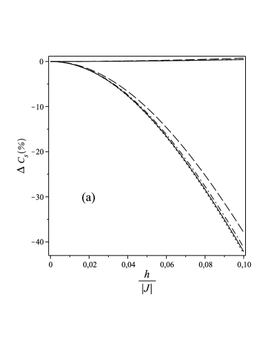
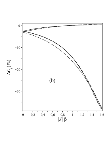
Figure 1: The percentage difference of the specific heat for $h=0$ and for a weak magnetic field $h$ for the AF ($J=1$) and for the ferromagnetic models ($J=-1$). Notice that for the AF case, all curves are close to the horizontal axis. This comparison is made for both models with $s=1/2$ (dashed line), $s=2$ (dash-dotted line), $s=4$ (solid line) and the large-spin limit model (dotted line). In figure 1 (a) this percentage difference is plotted as a function of ${h}/{|J|}$ with $D=0$ and $(|J|\beta)=1.6$. Figure 1 (b) presents the curves of $\Delta C_{s}$ versus $(|J|\beta)$ with ${D}/{|J|}=-0.5$ and ${h}/{|J|}=0.1$.

Let us compare the thermodynamic functions.

1) Comparison of the specific heat per site: $C_{s}(J,h,D;\beta)$.

For each spin-$s$, the specific heat functions of the ferromagnetic and AF models, in the high temperature limit ($\beta\rightarrow 0$), reach the same value for any $h$ and $D$. The $\beta^{2}$ term in this thermodynamic function has a $J^{2}$ dependence for both models.

Figure 1 show $\Delta C_{s}(\pm 1,{h}/{|J|},{D}/{|J|};|J|\beta)$ for $s=1/2,2,4$ and $\infty$ (large-spin limit model) as a function of ${h}/{|J|}$ and $(|J|\beta)$. In figure 1 (a) we have $D=0$, $|J|\beta=1.6$ and ${h}/{|J|}\in[0,0.1]$. For these spin values, $|\Delta C_{s}(-1,{h}/{|J|},0;1.6)\lesssim 43\%$ for the ferromagnetic models, whereas $|\Delta C_{s}(1,{h}/{|J|},0;1.6)|\lesssim 0.42\%$ for the AF models. In the AF case the function $\Delta C_{s}(1,{h}/{|J|},0;1.6)$ for $s=1/2$ very closely approximates its large-spin limit ($s\rightarrow\infty$) version. Figure 1 (b) shows the percentage difference $\Delta C_{s}$ as a function of $(|J|\beta$), for ${D}/{|J|}=-0.5$ and ${h}/{|J|}=0.1$. Again we have that the percentage differences of the ferromagnetic models are high ($|\Delta C_{s}(-1,0.1,-0.5;|J|\beta)|\lesssim 38\%$ whereas the percentage differences for the AF models are much smaller ($|\Delta C_{s}(1,0.1,-0.5;|J|\beta)|\lesssim 3\%$).

The previous discussion exemplifies the fact that the high-temperature expansion of the specific heat of the AF model in the presence of a weak longitudinal magnetic field can be approximated by the corresponding expression derived from the results of reference [13] (where we have $h=0$). Figure 1 shows us that for arbitrary spin-$s$ we can improve this approximation by recognizing that $C_{s}(1,{h}/{|J|},{D}/{|J|};|J|\beta)\approx C_{s}(1,0,{D}/{|J|};|J|\beta)+\Delta C_{1/2}(1,{h}/{|J|},{D}/{|J|};|J|\beta)$, at least in the region in which ${h}/{|J|}\ll 1$ and $|J|\beta\lesssim 1.6$. It is important to recall that the exact expression of $C_{1/2}(J,h,D;\beta)$ is known [14].

For the spin-$s$ ferromagnetic model (2) we need to know the high-temperature expansion of the HFE in the presence of longitudinal magnetic field to obtain the value of $C_{s}(-1,{h}/{|J|},{D}/{|J|};|J|\beta),$ even in the presence of a weak field.

2) Comparison of the correlation function between first neighbors per site: ${\mathcal{C}}_{s}(J,h,D;\beta)$.

Equation (14) tells us that in the absence of magnetic field ($h=0$),

$${\mathcal{C}}_{s}(-J,0,D;\beta)=-\;{\mathcal{C}}_{s}(J,0,D;\beta)$$ (16)

for $s=\frac{1}{2},1,\frac{3}{2},2,\ldots$ Result (16) describes the parallel (anti-parallel) alignment of the neighboring spins in the ferromagnetic (AF) model.

We want to check how the function ${\mathcal{C}}_{s}(\pm 1,{h}/{|J|},{D}/{|J|};|J|\beta)$ differs from the equality (16) in the presence of a weak magnetic field. In order to quantify this deviation, we define

$${\mathcal{D}}{\mathcal{C}}_{s}\left({h}/{|J|},{D}/{|J|};|J|\beta\right)\equiv\left[\frac{{\mathcal{C}}_{s}\left(-1,{h}/{|J|},{D}/{|J|};|J|\beta\right)+{\mathcal{C}}_{s}\left(1,{h}/{|J|},{D}/{|J|};|J|\beta\right)}{{\mathcal{C}}_{s}\left(-1,{h}/{|J|},{D}/{|J|};|J|\beta\right)}\right]\,\times\,100\%\,.$$ (17)

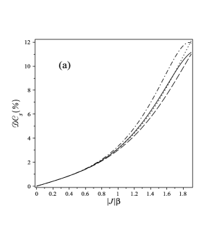
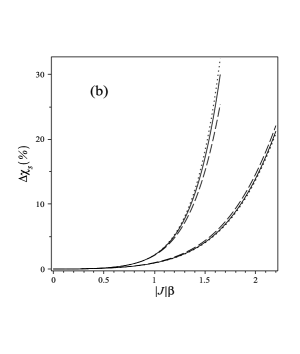
Figure 2: Left: comparison of the percentage function ${\mathcal{D}}{\mathcal{C}}_{s}$ for the $s=2$ and the large-spin limit ($s\rightarrow\infty$) models for ${h}/{|J|}=0.1$: for $s=2$, the cases $D=0$ (dashed line) and ${D}/{|J|}=-0.5$ (solid line) are shown, whereas for the $s\rightarrow\infty$ model the $D=0$ (dotted line) and ${D}/{|J|}=-0.5$ (dash-dotted line) cases are shown. Right: comparison of the percentage difference of the magnetic susceptibility $\Delta\chi_{s}(-1,0.1,D;\beta)$ in the ferromagnetic model ($J=-1$) for $s\in\{2,4,\infty\}$, for ${D}/{|J|}=-0.5$ (upper set of curves) and for ${D}/{|J|}=-0.5$ (lower set of curves); in both sets, the $s=2$ (dashed line), $s=4$ (solid line) and $s\rightarrow\infty$ (dotted line) cases are shown.

In figure 2 (a) we show the percentage function (17), with $D=0$ and ${D}/{|J|}=-0.5$, with ${h}/{|J|}=0.1$, to verify the departure from equation (16) for the ferromagnetic and AF models in the presence of a weak magnetic field. The function ${\mathcal{D}}{\mathcal{C}}_{s}({h}/{|J|},{D}/{|J|};|J|\beta)$ depends on the spin value and for lower temperatures ($|J|\beta\sim 1.9$) it can be around $~{}10\%$.

3) Comparison of the magnetic susceptibility per site: $\chi_{s}(J,h,D;\beta)$.

It is simple to obtain the high-temperature expansion of the magnetic susceptibility per site, $\chi_{s}(J,h,D;\beta)$, from the series (13) for the HFE $\left(\chi_{s}(\beta)=-{\partial^{2}{\mathcal{W}}_{s}(\beta)}/{\partial h^{2}}\right)$.

At $h=0$, the magnetic susceptibility of the ferromagnetic and AF models are distinct. We define a percentage difference analogous to equation (15) to present in figure 2 (b) the difference between $\chi_{s}(-1,0.1,{D}/{|J|};|J|\beta)$ and $\chi_{s}(-1,0,{D}/{|J|};|J|\beta)$ in the ferromagnetic models with $s=2,4$ and the large-spin limit model. In this figure we have ${D}/{|J|}=\pm 0.5$. For lower temperatures ($|J|\beta\sim 2)$ we have percentage differences around $20\%$. By looking at figure 2 (b) we see that for $J=-1$ we have ${\mathrm{d}(\Delta\chi_{s})}/{\mathrm{d}\beta}\big{|}_{D=-0.5}>{\mathrm{d}(\Delta\chi_{s})}/{\mathrm{d}\beta}\big{|}_{D=0.5}$ . This inequality is explained by the fact that for $D<0$ the states with the largest values of $\left(S_{i}^{z}\right)^{2}$ are more probable, whereas the states with the smallest values of $\left(S_{i}^{z}\right)^{2}$ are favored in the model with $D>0$.

For the AF models ($J=1$), in the interval $|J|\beta\in[0,1.43]$, with ${h}/{|J|}=0.1$ and ${D}/{|J|}=\pm 0.5$, we obtain from the percentage difference (15) $|\Delta\chi_{s}(1,0.1,{D}/{|J|};|J|\beta)|\lesssim 0.6\%$.

We point out that to derive the high-temperature expansion of $\chi_{s}(J,h,D;\beta)$ from the HFE, we need the dependence of the HFE on $h$. That is not the case of the previous paper on the spin-$S$ Ising model [7].

4 Thermodynamic behavior of the single-chain magnet in the interval $10~{}\text{K}\lesssim T\lesssim 40~{}\text{K}$

The Hamiltonian (1), with $S=3$, was applied by Kishine et al. [9] to analyze the low energy dynamics of the single-chain magnet (SCM) $[{\rm Mn(saltmen)}]_{2}[{\rm Ni(pao)}_{2}{\rm(py)}_{2}]{\rm(PF}_{6})_{2}$ for $T<40$ K in the presence of a weak magnetic field. Their Hamiltonian (2) is identical to ours (1) once we set $J^{\prime}=-2t$.

In [19] we studied the thermodynamics of the unitary spin-$s$ $XXZ$ model with a single-ion anisotropy term in the presence of a magnetic field in the $z$ direction. We obtained that the specific heat, the magnetization and the magnetic susceptibility of this model with $s=3$ are well approximated by their respective large-spin limit versions, in the temperature range of $|J|\beta\lesssim 1$. For the non-normalized $S=3$ $XXZ$ model this range corresponds to $|J|\beta\lesssim 0.083$ (see section 2.2 of reference [19]).

In this section, we compare the Hamiltonian (1) having spin-$3$ with its large-spin limit version for $T\lesssim 40$ K. By ‘‘large-spin limit model’’ we mean that the z component of its spin vector $\vec{S}$ varies continuously, namely, $S_{i}^{z}=2\sqrt{3}\cos(\theta_{i})$, in which $\theta_{i}\in[0,\pi]$, and $i\in\{1,2,\ldots,N\}$. In order to relate our analysis to the aforementioned SCM we use the same parameter values as in [9], namely,

$$\frac{J^{\prime}}{k}=-1.6~{}\text{K}$$ (18a)

and

$$\frac{D^{\prime}}{k}=-2.5~{}\text{K},$$ (18b)

in the spin-3 and large-spin limit Hamiltonians. One is reminded that $k$ is the Boltzmann constant. Taking the value (18a) for $J^{\prime}$, for $T\sim 40$ K we have $|J^{\prime}|\beta\sim 0.04$. Note that the temperature region characterized by $|J|\beta\lesssim 0.04$ is contained in the temperature region in which the spin-3 $XXZ$ model behaves very much like its large-spin limit version.

Along this section, we take ${h^{\prime}}/{k}=0.25$ K, which is a weak magnetic field (${h^{\prime}}/{|D^{\prime}|}=0.1$).

Let ${\mathcal{F}}_{S}(h;\beta)$ be a thermodynamic function. Its percentage difference of the $S=3$ and the large-spin limit models is defined as

$$\Delta{\mathcal{F}}(h;\beta)\equiv\left[\frac{{\mathcal{F}}_{S\rightarrow\infty}(h;\beta)-{\mathcal{F}}_{3}(h;\beta)}{{\mathcal{F}}_{S\rightarrow\infty}(h;\beta)}\right]\;\times\;100\%\,.$$ (19)

In figure 3 we plot the percentage difference (19) of the specific heat, the $z$ component of the magnetization per site $M_{z}^{(S)}(J^{\prime},h^{\prime},D^{\prime};\beta)$ $\left(M_{z}^{(S)}(\beta)\equiv-\frac{\partial{\mathcal{W}}_{S}(\beta)}{\partial h}\right)$ and the magnetic susceptibility per site. The dash-dotted curve corresponds to the specific heat in the interval $T\in[14.1~{}\text{K},40~{}\text{K}]$. For $T\lesssim 40$ K or $|J^{\prime}|\beta\gtrsim 0.046$, we verify that $\Delta C(0.25;\beta)\gtrsim 10\%$. The percentage difference of the $z$ component of the magnetization, $\Delta M_{z}(0.25;\beta)$, is given by the solid line in the figure for $T\in[11.63~{}\text{K},40~{}\text{K}]$, while the dotted curve describes $\Delta\chi(0.25;\beta)$ in the temperature window $T\in[12.99~{}\text{K},40~{}\text{K}]$. We verify that for $T\lesssim 19.3$ K, that is, $|J^{\prime}|\beta\gtrsim 0.083$, the $z$ component of the magnetization and the magnetic susceptibility of the spin-$3$ model of the SCM differ more than $8.5\%$ from their corresponding large-spin limit values.

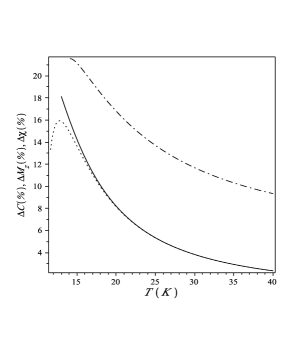
Figure 3: The percentage differences between the thermodynamic functions of the spin-$3$ model and its large-spin limit version of the SCM. The dash-dotted line corresponds to $\Delta C(0.25;\beta)$, the solid line to $\Delta M_{z}(0.25;\beta)$ and the dotted line to $\Delta\chi(0.25;\beta)$.

Due to the ratio ${|J^{\prime}|}/{|D^{\prime}|}$ value of $0.64$ for this SCM, the single-ion anisotropy term gives the main contribution to its thermodynamics. Since the crystal field $D^{\prime}$ is negative (see equation (18b)), the states with $S_{i}^{z}=\pm 3$ and $\pm 2$ are the most probable. The modulus of the amount of energy, in units of $k$, for the single-ion anisotropy term to change from states with $S_{i}^{z}=\pm 2$ to states with $S_{i}^{z}=\pm 3$, and vice-versa, is $12.5$ K. This value is close to one-third of 40 K. We conclude that for $T\lesssim 40$ K (that is, $|J^{\prime}|\beta\gtrsim 0.04$), the discretized nature of the spin-$3$ is still an important feature of the model. This result is very different from that of reference [19] for the spin-$3$ $XXZ$ model with a single-ion anisotropy term in the presence of a magnetic field in the $z$ direction.

Our expansion of the HFE with $S=3$ can be easily used to fit the experimental data of this SCM. It can also be applied to determine the best fit of the parameters $J^{\prime}$ and $D^{\prime}$.

5 Conclusions

The method of reference [12] permits one to calculate the high-temperature expansion of the HFE of any chain Hamiltonian with interaction between first neighbors which is invariant under space translation and satisfies a periodic space condition. If the Hamiltonian also satisfies the condition (8), we show that some of the terms that contribute to the function $H_{1,m}^{(n)}$ have already been calculated in a lower order of $n$, that is, $H_{1,m-1}^{(n-1)}$. A set of important 1D Hamiltonians satisfy the condition (8). This contribution from lower order of $n$ to this auxiliary function permits us to compute the HFE of the one-dimension Ising model with single-ion anisotropy term in the presence of a longitudinal magnetic field up to order $\beta^{17}$, for arbitrary values of spin $S$ and of the other parameters $J$, $h$ and $D$. Upon performing the numerical analysis of the thermodynamics of spin models (1) and (2) one must know the value of the spin beforehand.

We discuss the thermodynamics of the normalized Hamiltonian (see equation (2)), but equation (7) relates the HFE of the Hamiltonian (1) and its normalized version (equation (2)).

Some thermodynamic functions are insensitive to the sign of $J$ in the absence of a magnetic field; for instance, the specific heat of the ferromagnetic ($J<0$) and AF ($J>0$) spin-$S$ Ising models with single-ion anisotropy term are identical with $h=0$. In the absence of a magnetic field, the ferromagnetic model favors parallel neighboring spins while in the AF model the anti-parallel pairs are more probable. The effect of the presence of an external magnetic field in both models is that of favoring the alignment of spins at each site to the field direction. In the ferromagnetic model such alignment is favored by the coupling between neighboring spins. On the other hand, in the AF model there is a competition between the coupling of neighboring spins (favoring anti-parallel alignment) and the Zeeman term (forcing all the spins in the chain to align with the external magnetic field). As a consequence of this competition, there is a perturbative effect in the AF model due to the presence of a weak magnetic field; in such regime, their thermodynamic functions ${\mathcal{F}}_{s}(1,{h}/{|J|},{h}/{|J|};|J|\beta)$ for the spin-$s$ model can be approximated by ${\mathcal{F}}_{s}(1,{h}/{|J|},{D}/{|J|};|J|\beta)\approx{\mathcal{F}}_{s}(1,0,{D}/{|J|};|J|\beta)+\Delta{\mathcal{F}}_{1/2}(1,{h}/{|J|},{h}/{|J|};|J|\beta)$. The exact expression of the HFE of the spin-$1/2$ Ising model with a single-ion anisotropy term in the presence of a longitudinal magnetic field is known [14]. In the ferromagnetic model, the effect of the Zeeman coupling cannot be treated anymore as a perturbation to the interaction between first neighbors and to the single-ion anisotropy term for ${h}/{|J|}\gtrsim 0.04$.

Kishine et al. [9] applied the spin-$3$ Hamiltonian (1) to analyse the low energy dynamics of the ${\rm[Mn(saltmen)]_{2}[Ni(pac)_{2}(py)_{2}](PF_{6})_{2}}$ SCM for temperatures $T<40$ K. Although $S=3$ could be considered a high spin value in the region of $T\sim 40$ K ($|J^{\prime}|\beta\sim 0.04$), the negative value of $D^{\prime}$ favors the states with $S_{i}^{z}=\pm 2$ and $\pm 3$. The modulus of the amount of energy required by the single-ion anisotropy term to have $S_{z}$ varied from $\pm 2\rightleftharpoons\pm 3$ and vice-versa is about one-third of the thermal energy available for $T\lesssim 40$ K. Our results show that the large-spin limit model, with the spin-3 replaced by the classical vector in the Hamiltonian, yields a poor approximation to the behavior of this SCM for $T\lesssim 18$ K and for the set of parameters values (18a) and (18b).

Finally, it is very important to point out that our high-temperature expansion of the HFE of the spin-$s$ Ising model can be applied to fit experimental data of new materials with one-dimensional behavior and strong anisotropy axis. This expansion leaves the spin value of the material as one of the parameters to be determined by the best fit. The expansion is valid for positive and negative values of $J$ and $D$ in the presence of a longitudinal magnetic field that does not have to be a weak field.

Ukrainian 0

Високотемпературний розклад для класичної моделi Iзiнга iз членом $S_{z}^{2}$

М.Т. Томас${}^{\textsf{\footnotesize{\mbox{?}}}}$, О. Рохас${}^{\textsf{\footnotesize{\mbox{?}}}}$

             
${}^{\textsf{\footnotesize 1}}$ Iнститут фiзики, Федеральний унiверситет Флумiненсе, Нiтерой-RJ, Бразилiя ${}^{\textsf{\footnotesize 2}}$ Факультет точних наук, Федеральний унiверситет м. Лаврас, Лаврас-MG, Бразилiя

References

- [1] Ising E., Z. Phys., 1925, 31, 253; doi:10.1007/BF02980577.
- [2] Baxter R.J., Exactly Solved Models in Statistical Mechanics, Academic Press, London, 1989, section 2.1.
- [3] Krinsky S., Furman D., Phys. Rev. B, 1975, 11, 2602; doi:10.1103/PhysRevB.11.2602.
- [4] Mancini F., Europhys. Lett., 2005, 70, 485; doi:10.1209/epl/i2005-10016-4.
- [5] Mancini F., Mancini F.P., Condens. Matter Phys., 2008, 11, 543.
- [6] Avella A., Mancini F., Eur. Phys. J. B, 2006, 50, 527; doi:10.1140/epjb/e2006-00177-x.
- [7] Rojas O., de Souza S.M., Moura-Melo W.A., Physica A, 2007, 373, 324; doi:10.1016/j.physa.2006.05.055.
- [8] Ni Z.-H., Zhang L.F., Tangoulis V., Wernsdorfer W., Cui A.L., Sato O., Kou H.Z., Inorg. Chem., 2007, 46, 6029; doi:10.1021/ic700528a and references therein.
- [9] Kishine J.-i., Watanabe T., Deguchi H., Mito M., Sakai T., Tajiri T., Yamashita M., Miyasaka H., Phys. Rev. B, 2006, 74, 224419; doi:10.1103/PhysRevB.74.224419.
- [10] Blume M., Phys. Rev., 1966, 141, 517; doi:10.1103/PhysRev.141.517.
-
[11]
Capel H.W., Physica, 1966, 32, 966; doi:10.1016/0031-8914(66)90027-9;
Capel H.W., Physica, 1967, 33, 295; doi:10.1016/0031-8914(67)90167-X. - [12] Rojas O., de Souza S.M., Thomaz M.T., J. Math. Phys., 2002, 43, 1390; doi:10.1063/1.1432484.
- [13] Moura-Melo W.A., Rojas O., Correa Silvad E.V., de Souza S.M., Thomaz M.T., Physica A, 2003, 322, 393; doi:10.1016/S0378-4371(02)01749-1. (Please notice a misprint under the square root in equation (28): the factor should read .)
-
[14]
Rojas O., de Souza S.M., Correa Silva E.V., Thomaz M.T., Braz. J. Phys., 2001, 31, 577;
doi:10.1590/S0103-97332001000400008. (Please notice a misprint in the HFE of this reference: the constant in equation (25) should read .) - [15] Heisenberg W., Z. Physik, 1928, 49, 619; doi:10.1007/BF01328601.
- [16] Takahashi M., Thermodynamics of One-Dimensional Solvable Models, Cambridge Univ. Press, 1999, chapter 4.
-
[17]
Hubbard J., Proc. R. Soc. Lond. A, 1963, 276, 238; doi:10.1098/rspa.1963.0204;
Hubbard J., Proc. R. Soc. Lond. A, 1964, 281, 401; doi:10.1098/rspa.1964.0190;
Gutzwiller M., Phys. Rev. Lett., 1963, 10, 159; doi:10.1103/PhysRevLett.10.159;
Gutzwiller M., Phys. Rev., 1965, A137, 1726; doi:10.1103/PhysRev.137.A1726. - [18] Essler F.H.L., Frahm H., Göhmann F., Klümper A., Korepin V.E., The One-Dimensional Hubbard Model, Cambridge Univ. Press, 2010.
-
[19]
Rojas O., de Souza S.M., Correa Silva E.V., Thomaz M.T., Eur. Phys. J. B, 2005, 47, 165;
doi:10.1140/epjb/e2005-00310-5.
Ukrainian \adddialect\l@ukrainian0 \l@ukrainian