Trajectory and stability of Lagrangian point $L_{2}$ in the Sun-Earth system

Abstract

This paper describes design of the trajectory and analysis of the stability of collinear point $L_{2}$ in the Sun-Earth system. The modified restricted three body problem with additional gravitational potential from the belt is used as the model for the Sun-Earth system. The effect of radiation pressure of the Sun and oblate shape of the Earth are considered. The point $L_{2}$ is asymptotically stable upto a specific value of time $t$ correspond to each set of values of parameters and initial conditions. The results obtained from this study would be applicable to locate a satellite, a telescope or a space station around the point $L_{2}$.

1 Introduction

This paper deals with the Sun-Earth system with the modified restricted three body problem model[as in Kushvah (2009a, b)] including radiation pressure, oblateness of the Earth and influence of the belt. Further it considered that the primary bodies are moving in circular orbits about their center of mass. It is well-known that five equilibrium points(Lagrangian points) that appear in the planar restricted three-body problem are very important for astronautical applications. The collinear points are unstable and the triangular points are conditionally stable in the classical restricted three body problem[please see Szebehely (1967)]. This can be seen in the Sun-Jupiter system where several thousand asteroids(collectively referred to as Trojan asteroids), are in orbits of triangular equilibrium points. But collinear equilibrium points are also made linearly stable by continuous corrections of their orbits(“halo orbits”). In other words the collinear equilibrium points are metastable points in the sense that, like a ball sitting on top of a hill. However, in practice these Lagrange points have proven to be very useful indeed since a spacecraft can be made to execute a small orbit about one of these Lagrange points with a very small expenditure of energy[please see Farquhar (1967, 1969)].

We considered the Chermnykh’s problem which is a new kind of restricted three body problem, it was first time studied by Chermnykh (1987). This problem generalizes two classical problems of Celestial mechanics: the two fixed center problem and the restricted three body problem. This gives wide perspectives for applications of the problem in celestial mechanics and astronomy. The importance of the problem in astronomy has been addressed by Jiang and Yeh (2004a). Some planetary systems are claimed to have discs of dust and they are regarded to be young analogues of the Kuiper Belt in our Solar System. If these discs are massive enough, they should play important roles in the origin of planets’orbital elements. Since the belt of planetesimal often exists within a planetary system and provides the possible mechanism of orbital circularization, it is important to understand the solutions of dynamical systems with the planet-belt interaction.The Chermnykh’s problem has been studied by many scientists such as Jiang and Yeh (2004b), Papadakis (2004),Papadakis (2005) and Jiang and Yeh (2006); Yeh and Jiang (2006).

The present paper investigates the nature of collinear equilibrium point $L_{2}$ because of the interested point to locate an artificial satellite. Although there are two new equilibrium points due to mass of the belt(larger than 0.15) as obtained by Jiang and Yeh (2006); Yeh and Jiang (2006), but they are left to be examined. All the results are computed numerically using same technique as in Grebennikov and Kozak-Skoworodkin (2007), because pure analytical methods are not suitable. For specific time intervals, and initial values, these results provide new information on the behavior of trajectories around the Lagrangian point $L_{2}$.

2 Location of the Lagrangian Points

It is supposed that the motion of an infinitesimal mass particle is influenced by the gravitational force from primaries and a belt of mass $M_{b}$. The units of the mass and the distance are taken such that sum of the masses and the distance between primaries are unities. The unit of the time i.e. the time period of $m_{1}$ about $m_{2}$ consists of $2\pi$ units such that the Gaussian constant of gravitational $\mathbf{k}^{2}=1$. Then perturbed mean motion $n$ of the primaries is given by $n^{2}=1+\frac{3A_{2}}{2}+\frac{2M_{b}r_{c}}{\left(r_{c}^{2}+T^{2}\right)^{3/2}}$, where $T=\mathbf{a}+\mathbf{b}$, $\mathbf{a,b}$ are flatness and core parameters respectively which determine the density profile of the belt. $r_{c}^{2}=(1-\mu)q_{1}^{2/3}+\mu^{2}$, $A_{2}=\frac{r^{2}_{e}-r^{2}_{p}}{5r^{2}}$ is the oblateness coefficient of $m_{2}$; $r_{e}$, $r_{p}$ are the equatorial and polar radii of $m_{2}$ respectively. $r=\sqrt{x^{2}+y^{2}}$ is the distance between primaries and $x=f_{1}(t),y=f_{2}(t)$ are the functions of time $t$ i.e. $t$ is only independent variable. The mass parameter is $\mu=\frac{m_{2}}{m_{1}+m_{2}}$($9.537\times 10^{-4}$ for the Sun-Jupiter and $3.00348\times 10^{-6}$ for the Sun-Earth mass distributions respectively ). $q_{1}=1-\frac{F_{p}}{F_{g}}$ is a mass reduction factor, where $F_{p}$ is the solar radiation pressure force which is exactly apposite to the gravitational attraction force $F_{g}$. The coordinates of $m_{1}$, $m_{2}$ are $(-\mu,0)$, $(1-\mu,0)$ respectively. In the above mentioned reference system and Miyamoto and Nagai (1975) model, the equations of motion of the infinitesimal mass particle in the $xy$-plane formulated as[please see Kushvah (2008),Kushvah (2009a)]:

$$\ddot{x}-2n\dot{y} = \Omega_{x},$$ (1)

$$\ddot{y}+2n\dot{x} = \Omega_{y},$$ (2)

where

$$\Omega_{x} = n^{2}x-\frac{(1-\mu)q_{1}(x+\mu)}{r^{3}_{1}}-\frac{\mu(x+\mu-1)}{r^{3}_{2}}-\frac{3}{2}\frac{\mu{A_{2}}(x+\mu-1)}{r^{5}_{2}}$$

$$-\frac{M_{b}x}{\left(r^{2}+T^{2}\right)^{3/2}},$$

$$\Omega_{y} = n^{2}y-\frac{(1-\mu)q_{1}{y}}{r^{3}_{1}}-\frac{\mu{y}}{r^{3}_{2}}-\frac{3}{2}\frac{\mu{A_{2}}y}{r^{5}_{2}}-\frac{M_{b}y}{\left(r^{2}+T^{2}\right)^{3/2}},$$

$$\Omega = \frac{n^{2}(x^{2}+y^{2})}{2}+\frac{(1-\mu)q_{1}}{r_{1}}+\frac{\mu}{r_{2}}+\frac{\mu A_{2}}{2r_{2}^{3}}+\frac{M_{b}}{\left(r^{2}+T^{2}\right)^{1/2}},$$ (3)

$$r_{1} = \sqrt{(x+\mu)^{2}+y^{2}},r_{2}=\sqrt{(x+\mu-1)^{2}+y^{2}}.$$

From equations (1) and (2), the Jacobian integral is given by:

$$E=\frac{1}{2}\left(\dot{x^{2}}+\dot{y}^{2}\right)-\Omega(x,y,\dot{x},\dot{y})=(\mbox{Constant}),$$ (4)

which is related to the Jacobian constant $C=-2E$. The location of three collinear equilibrium points and two triangular equilibrium points is computed by dividing the orbital plane into three parts $L_{1},L_{4(5)}$: $\mu<x<(1-\mu)$, $L_{2}$: $(1-\mu)<x$ and $L_{3}$: $x<-\mu$. For the collinear points, an algebraic equation of the fifth degree is solved numerically with initial approximations to the Taylor-series as:

$$x(L_{1}) = 1-(\frac{\mu}{3})^{1/3}+\frac{1}{3}(\frac{\mu}{3})^{2/3}-\frac{26\mu}{27}+\dots,$$ (5)

$$x(L_{2}) = 1+(\frac{\mu}{3})^{1/3}+\frac{1}{3}(\frac{\mu}{3})^{2/3}-\frac{28\mu}{27}+\dots,$$ (6)

$$x(L_{3}) = -1-\frac{5\mu}{12}+\frac{1127\mu^{3}}{20736}+\frac{7889\mu^{4}}{248832}+\dots.$$ (7)

The solution of differential equations (1) and (2) is presented as interpolation function which is plotted for various integration intervals by substituting specific values of the time $t$ and initial conditions i.e. $x(0)=x(L_{i}),y(0)=0$ where $i=1-3$ and $x(0)=\frac{1}{2}-\mu,y(0)=\pm\frac{\sqrt{3}}{2}$ (for the triangular equilibrium points).

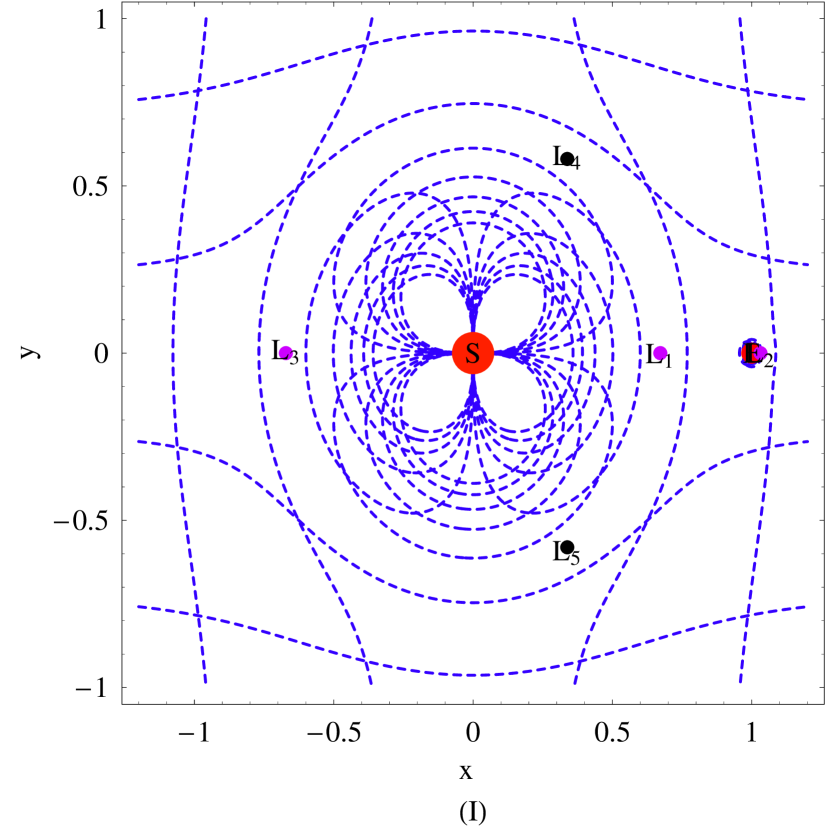
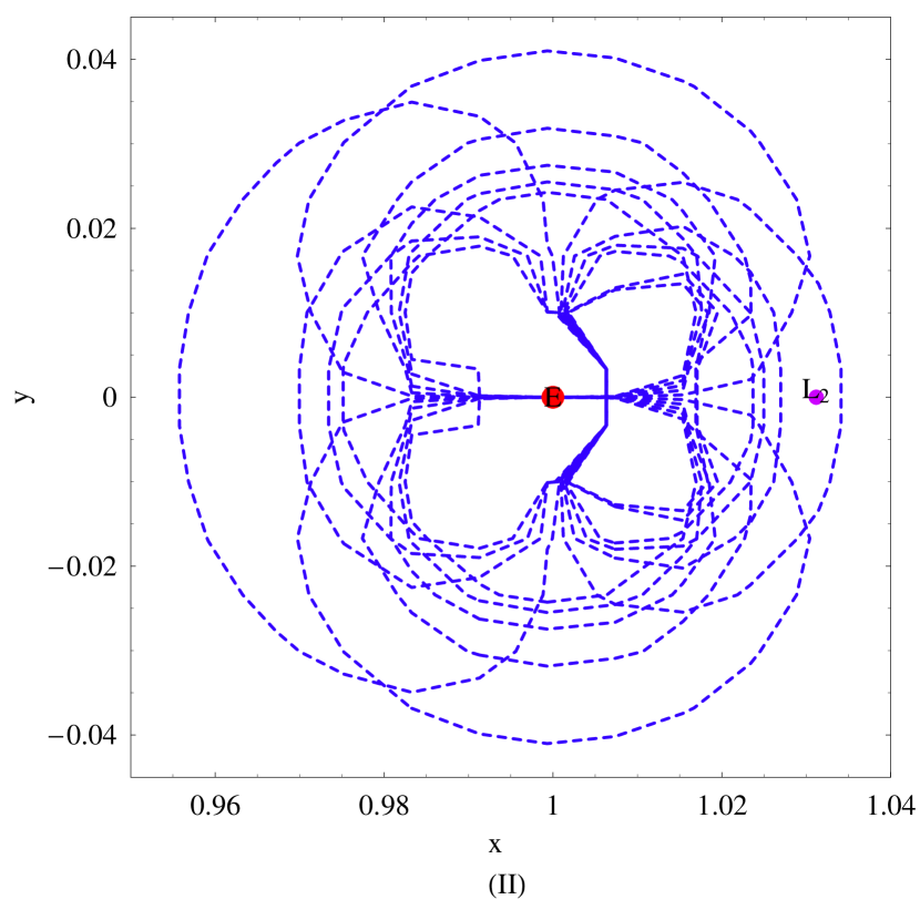
Figure 1: The position of equilibrium points when T=0.1, $q_{1}=0.5$, $A_{2}=0.25$ and $M_{b}=0.25$, panel (I): Pink points are collinear points and black points are triangular points (II): Position of $L_{2}$ with respect to Earth is shown in zoom.

The equilibrium points are shown in figure 1 in which two panels i.e. (I) pink points correspond to the collinear points and black points correspond to the triangular points for the Sun-Earth system, whereas panel (II) show the zoom of the neighborhood of $L_{2}$. The numerical values of these points are presented in Table 1. It is seen that the positions of $L_{1},L_{3}$ are shifted to rightward; $L_{2},L_{4}$ are shifted to leftward; and $L_{4}$ is also shifted to downward with respect to their positions in the classical problem. The nature of the $L_{5}$ is not discussed in present model because it is same as the nature of $L_{4}$. But the detail behavior of the $L_{2}$ with stability regions is discussed in sections 3 & 4.

Table 1: Location of equilibrium points, when $T=0.1$, $A_{2}=0.25$ and $M_{b}=0.25$.

$q_{1}=0.75$			$q_{1}=0.5$
$L_{i}$	x	y	x	y
$L_{1}$	0.844989	0	0.671768	0
$L_{2}$	1.03519	0	1.03118	0
$L_{3}$	-0.845423	0	-0.671796	0
$L_{4}$	0.419679	0.733898	0.337923	0.580616

2.1 Comments on the Parameters

However,in general, it might be difficult to know the critical values of the parameters, but they could be obtained with the help of Interval Arithmetic(IA), which was introduced by Moore (1963). As per the IA, if $I_{a}=[a_{1},a_{2}],I_{b}=[b_{1},b_{2}]$ be two intervals, then four basic arithmetic operations can be defined as:

• Sum: $I_{1}+I_{2}=[a_{1}+b_{1},a_{2}+b_{2}]$.

• Difference: $I_{1}-I_{2}=[a_{1}-b_{2},a_{2}-b_{1}]$.

• Product: $I_{1}\times I_{2}=[\mbox{min}(a_{1}b_{1},a_{1}b_{2},a_{2}b_{1},a_{2}b_{2}),\mbox{max}(a_{1}b_{1},a_{1}b_{2},a_{2}b_{1},a_{2}b_{2})]$.

• Division: $I_{1}/I_{2}=[\mbox{min}(a_{1}/b_{1},a_{1}/b_{2},a_{2}/b_{1},a_{2}/b_{2}),\mbox{max}(a_{1}/b_{1},a_{1}/b_{2},a_{2}/b_{1},a_{2}/b_{2})]$. The division by an interval containing zero is not defined in basic IA, so this case is avoided.

It is supposed that mass of the Sun $m_{1}$ is greater than mass of the Earth $m_{2}$, therefore $m_{1}\leq m_{1}+m_{2}$ and $m_{2}\leq m_{1}+m_{2}$. In other words, $m_{1}$ lies in $[\epsilon_{1},m_{1}+m_{2}]$ and $m_{2}$ lies in $[\epsilon_{2},m_{1}+m_{2}]$, where $\epsilon_{1}\geq\epsilon_{2}\geq 0$. Using relation $\mu=\frac{m_{2}}{m_{1}+m_{2}}$, the domain of mass parameter can be obtained as:

$$\mu\in\frac{[\epsilon_{2},m_{1}+m_{2}]}{[\epsilon_{1},m_{1}+m_{2}]+[\epsilon_{2},m_{1}+m_{2}]},$$ (8)

or $$\mu\in\left[\frac{\epsilon_{2}}{2},\frac{m_{1}+m_{2}}{2}\right].$$ (9)

From relation $r_{c}^{2}=(1-\mu)q_{1}^{2/3}+\mu^{2}$, the domain of mass reduction factor $q_{1}$ is given as:

$$q_{1}^{2/3}\in\left[\frac{\epsilon_{2}^{2}-(m_{1}+m_{2})^{2}}{1-\frac{(m_{1}+m_{2})}{2}},\frac{r^{2}-\epsilon_{2}^{2}}{1-\frac{(m_{1}+m_{2})}{2}}\right].$$ (10)

And from relation $A_{2}=\frac{r^{2}_{e}-r^{2}_{p}}{5r^{2}}$, where $r_{e}\in[\epsilon_{4},r]$ and $r_{e}\in[\epsilon_{5},r]$, $\epsilon_{4}\geq\epsilon_{5}\geq 0$. The domain of oblateness coefficient can be obtained as:

$$A_{2}\in\frac{[\epsilon_{4},r]^{2}-[\epsilon_{5},r]^{2}}{5r^{2}}$$ (11)

or $$A_{2}\in\left[\frac{\epsilon_{4}^{2}}{5r^{2}}-\frac{1}{5},\frac{1}{5}-\frac{\epsilon_{5}^{2}}{5r^{2}}\right]$$ (12)

Now from relation $n^{2}=1+\frac{3A_{2}}{2}+\frac{2M_{b}r_{c}}{\left(r_{c}^{2}+T^{2}\right)^{3/2}}$, $n\in[0,2]$, $T=0.1$, then the domain of $M_{b}$ is obtained as $[0,\frac{33(r+0.01)^{3/2}}{20r}]$. In particular if $\epsilon_{i}=0(i=1,2,3,4,5)$, $m_{1}+m_{2}=1$ (unit of mass), $r_{c}=r=1$(unit of distance), then it is obtained $\mu\in[0,\frac{1}{2}]$, $q_{1}\in[-2\sqrt{2},2\sqrt{2}]$, $A_{2}\in\left[-\frac{1}{5},\frac{1}{5}\right]$, and $M_{b}\in[0,1.6748]$. But in the present model it is considered that $0\leq F_{p}\leq F_{g}$, $r_{e}\geq r_{p}$, so definitely $q_{1}$ lies in [0,1], $A_{2}\in[0,1/5]$ i.e $A_{2}=2.4337\times 10^{-12}$.

3 Trajectory of $L_{2}$

The equations (1-2) with initial conditions $x(0)=x(L_{2}),y(0)=0,x^{\prime}(0)=y^{\prime}(0)=0$ are used to determine the trajectories of $L_{2}$ for different possible cases. For plotting of the figures, the position of $L_{2}$ at $t=0$ is considered as the origin of coordinate axes. The figure 2 show the trajectories of $L_{2}$ with four panels when $q_{1}=1,M_{b}=0.25,A_{2}=0$. The panels (I-II): describe the case $0<t<927.3$. In panel(I) trajectory is moving chaotically around the $L_{2}$ with $x\in(-1.66639,1.66663)$, $y\in(-1.66885,1.6708)$ and in panel (II) the energy integral $E$ is oscillating with negative values(approximate value is -1.99804). The panels (III-IV) are plotted for $927\leq t\leq 933$ for which the trajectory departs from the point and energy integral becomes negative for $t<929.9$, after this time it becomes positive. The maximum value of $E$ is 43.8974(at $t$=931.5). Also, when $t>931.5$ then $E$ is found strictly decreasing.

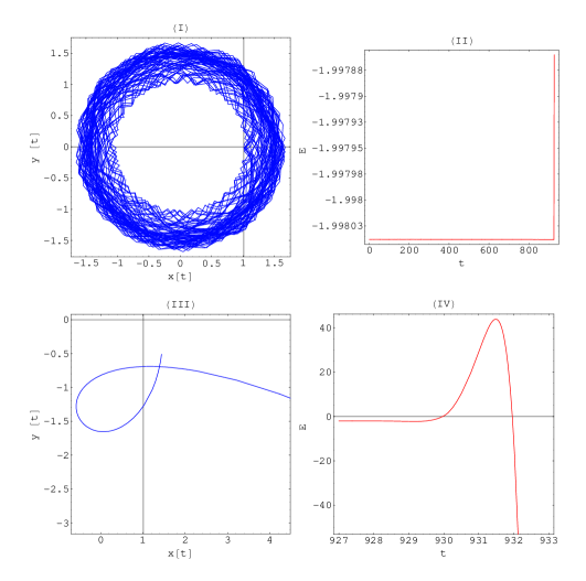
Figure 2: The Panels (I-II):$0<t<927.3$ and (III-VI):$927.3<t<933$ in which (I and III) show the trajectory of $L_{2}$, (II and IV) show energy-versus time, when T=0.1, $q_{1}=1$, $A_{2}=0$ and $M_{b}=0.25$.

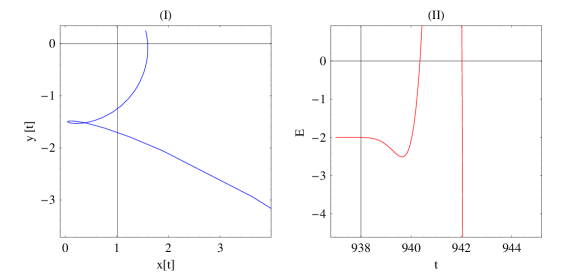
Figure 3: The Panels (I-II):$937<t<945$ in which (I) show the trajectory of $L_{2}$, (II) show energy-versus time when T=0.1, $q_{1}=1$, $A_{2}=0.0004$ and $M_{b}=0.25$.

The effect of Earth oblateness to the trajectory of $L_{2}$ is shown in figure 3 which is plotted for $q_{1}=1,M_{b}=0.25$ and $A_{2}=0.0004$. The behaviour of trajectory is almost same as in above case, and integral of energy is negative for $0<t<937.47$. It is clear from panels (I-II) the trajectory moves away from the Lagrangian point $L_{2}$ when $t\geq 940$. Initially energy integral has negative values for time $0\leq t\leq 940$ and it becomes positive for time $940\leq t\leq 942.02$, which attains maxima $E=25.2749$ at $t=941.6$, if $t\geq 942.03$ then $E<0$ is found.

Table 2: Maximum value of time $t_{m}$ for which trajectory of $L_{2}$ moves around the point when $A_{2}=10^{-j}$, pair ($q_{1},M_{b}$).

j	(1,0)	(1,0.25)	(1,0.50)	(0.75,0)	(0.75,0.25)	(0.75,0.50)	(0.50,0)	(0.50,0.25)	(0.50,0.50)
-10	1331.93101	922.79781	788.32512	180.74391	503.43326	505.77125	808.57010	420.18206	409.85720
-9	1293.30457	922.27673	790.59409	194.76252	681.94769	520.06460	420.18206	420.60738	401.85174
-8	1298.97760	921.81836	785.85800	419.97449	505.87022	521.37550	407.38452	407.38452	394.22863
-7	1245.34016	927.64717	787.31619	652.84935	656.81667	535.30463	414.11940	414.11940	405.16373
-6	1270.43530	929.71580	789.17206	606.81842	600.2735	521.63088	423.85070	423.85070	406.16332
-5	1.21501	929.21181	787.05192	388.61276	638.00066	537.18908	424.55070	424.55069	399.15415
-4	0.43533	924.27518	89.10469	596.68529	594.73322	516.01512	403.91467	403.91466	399.15415
-3	0.13977	0.18754	790.81103	0.18391	542.68447	493.82489	394.12204	394.12204	422.23115
-2	0.04427	0.045214	0.04624	0.04517	0.047163	0.04951	0.05098	0.05098	0.05088
-1	0.01400	0.01403	0.01406	0.01403	0.01408	0.01414	0.01417	0.01417	0.01417

The details of trajectory and energy are presented in Table 2 for various values of parameters and the effect of parameters on the stability is presented in Table 3, when $A_{2}=2.4337\times 10^{-12}$(for Sun-Earth system). One can see that maximum value $t_{m}$ of time for which trajectory moves around the points, which is an decreasing function of $M_{b}$. When $A_{2}$ is very small in ($10^{-10}-10^{-3}$) the value of $t_{m}$ is initially decreasing function of $A_{2}$ and increasing function of $q_{1}$. It is obtained that the value of $t_{m}$ is very small when $A_{2}>10^{-2}$.

4 Stability of $L_{2}$

Suppose the coordinates $(x_{1},y_{1})$ of $L_{2}$ are initially perturbed by changing $x(0)=x_{1}+\epsilon\cos(\phi),y(0)=y_{1}+\epsilon\sin(\phi)$, where

$$\phi=\arctan\left(\frac{y(0)-y_{1}}{x(0)-x_{1}}\right)\in(0,2\pi),$$

$0\leq\epsilon=\sqrt{(x(0)-x_{1})^{2}+(y(0)-y_{1})^{2}}<1$, and $\phi$ indicates the direction of the initial position vector in the local frame. If the $\epsilon=0$ means there is no perturbation. It is supposed that the $\epsilon=0.001$ and the $\phi=\frac{\pi}{4}$ to examine the stability of $L_{2}$. Figure 4 show the path of test particle and its energy with four panels i.e. the panels (I&III):$q_{1}=0.75,0.50,A_{2}=0.0$, in (I) trajectory of perturbed $L_{2}$ moves in chaotic-circular path around initial position without deviating far from it, then steadily move out of the region. It is found that the test particle moves in the stability region and returns repeatedly on its initial position. The blue solid curves represent $M_{b}=0.25$, for panel(I) $t\leq 530$ and for panel (II) $t\leq 425$. The red dashed curves represent $M_{b}=0.50$, for panel(III) $t\leq 510$ and panel (IV) $t\leq 350$.

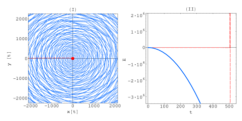
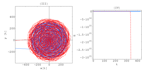
Figure 4: Panels (I & III) show the stability regions of $L_{2}$ (II & IV ) show the energy-versus time when T=0.1, $q_{1}=0.75,0.50$, $A_{2}=0.00$.

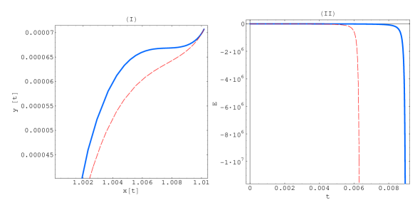
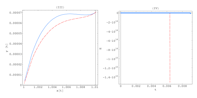
Figure 5: Show the stability of $L_{2}$ with panels (I-II):$q_{1}=0.75,M_{b}=.25$ and (III-IV):$q_{1}=0.50,M_{b}=0.25$ in which blue solid curves for $A_{2}=0.25$, red curves for $A_{2}=0.50$ when $T=0.1$.

The effect of oblateness of the second primary is shown in figure 5 when $q_{1}=0.75,M_{b}=0.25$. The panels (I&III) show the trajectory of perturbed point $L_{2}$ and (II&IV) show the energy of that point. The blue solid lines correspond to $A_{1}=0.25$ and red dashed lines correspond to $A_{2}=0.50$. One can see that the oblate effect is very powerful on the trajectory and on the stability of $L_{2}$. When $A_{2}$ is very small the $L_{2}$ is asymptotically stable for the value of $t$ which lies within a certain interval. But if oblate effect of second primary is grater than $10^{-2}$, the stability region of $L_{2}$ disappears.

Table 3: Time $t_{m}$ for the stability of $L_{2}$ when $T=0.1$, $A_{2}=2.4337\times 10^{-12}$

$q_{1}$	$M_{b}$=0.0	$M_{b}$=0.20	$M_{b}=0.40$	$M_{b}=0.60$	$M_{b}=0.80$	$M_{b}=1.00$
1.00	1330.94105	898.46095	740.63037	612.37135	476.86492	338.8331
0.90	822.12754	846.66095	695.75819	475.72650	384.90335	315.45105
0.80	872.68679	680.99491	577.52196	428.50822	357.90646	320.62530
0.70	645.16838	563.21770	581.43694	388.86721	355.88230	313.83184
0.60	599.14033	534.73979	446.02727	379.57860	350.15274	326.96167
0.50	821.08169	559.32274	432.84188	381.03250	343.84316	320.76820
0.40	720.76190	95.04409	429.40509	380.36035	343.26450	317.89680
0.30	651.26546	491.31201	425.49945	397.40864	333.97100	307.68910
0.20	640.84770	485.92301	435.45741	379.56781	344.58453	317.24080
0.10	609.87381	505.53178	413.39252	379.19007	328.82013	313.27721
0.00	600.63232	478.59863	416.37905	390.05165	334.88598	308.42592

5 Conclusion

The numerical computation presented in the manuscript provides remarkable results to design trajectories of Lagrangian point $L_{2}$ which helps us to make comments on the stability(asymptotically) of the point. We obtained the intervals of the time where trajectory continuously moves around the $L_{2}$, does not deviate far from the point but tend to approach (for some cases) it, the energy of perturbed point is negative for these intervals, so we conclude that the point is asymptotically stable. More over we have seen that after the specific time intervals the trajectory of perturbed point departs from the neighborhood and goes away from it, in this case the energy also becomes positive, so the Lagrangian point $L_{2}$ is unstable. Further the trajectories and the stability regions are affected by the radiation pressure, the oblateness of the second primary and mass of the belt.

References

- Chermnykh (1987) Chermnykh, S. V., 1987. Stability of libration points in a gravitational field. Vest. Leningrad Mat. Astron. 2, 73–77.
- Farquhar (1967) Farquhar, R. W., Oct. 1967. Lunar Communications with Libration-Point Satellites. Journal of Spacecraft and Rockets 4, 1383–1384.
- Farquhar (1969) Farquhar, R. W., 1969. Future Missions for Libration-Point Satellites. Astronautics Aeronautics, 52–56.
- Grebennikov and Kozak-Skoworodkin (2007) Grebennikov, E. A., Kozak-Skoworodkin, D., Sep. 2007. Numerical estimates for stability domains of Lagrangian solutions to the restricted three-body problem. Computational Mathematics and Mathematical Physics 47, 1477–1488.
- Jiang and Yeh (2004a) Jiang, I., Yeh, L., Sep. 2004a. Dynamical Effects from Asteroid Belts for Planetary Systems. International Journal of Bifurcation and Chaos 14, 3153–3166.
- Jiang and Yeh (2004b) Jiang, I.-G., Yeh, L.-C., Aug. 2004b. On the Chaotic Orbits of Disk-Star-Planet Systems. AJ128, 923–932.
- Jiang and Yeh (2006) Jiang, I.-G., Yeh, L.-C., Dec. 2006. On the Chermnykh-Like Problems: I. the Mass Parameter = 0.5. Ap&SS305, 341–348.
- Kushvah (2008) Kushvah, B. S., Nov. 2008. Linear stability of equilibrium points in the generalized photogravitational Chermnykh’s problem. Ap&SS318, 41–50.
- Kushvah (2009a) Kushvah, B. S., Sep. 2009a. Linearization of the Hamiltonian in the generalized photogravitational Chermnykh’s problem. Ap&SS323, 57–63.
- Kushvah (2009b) Kushvah, B. S., Sep. 2009b. Poynting-Robertson effect on the linear stability of equilibrium points in the generalized photogravitational Chermnykh’s problem. Research in Astronomy and Astrophysics 9, 1049–1060.
- Miyamoto and Nagai (1975) Miyamoto, M., Nagai, R., 1975. Three-dimensional models for the distribution of mass in galaxies. PASJ27, 533–543.
- Moore (1963) Moore, R. E., 1963. Interval arithmetic and automatic error analysis in digital computing. Ph.D. thesis, Stanford, CA, USA.
- Papadakis (2004) Papadakis, K. E., Oct. 2004. The 3D restricted three-body problem under angular velocity variation. A&A425, 1133–1142.
- Papadakis (2005) Papadakis, K. E., Sep. 2005. Motion Around The Triangular Equilibrium Points Of The Restricted Three-Body Problem Under Angular Velocity Variation. Ap&SS299, 129–148.
- Szebehely (1967) Szebehely, V., 1967. Theory of orbits. The restricted problem of three bodies. New York: Academic Press.
- Yeh and Jiang (2006) Yeh, L.-C., Jiang, I.-G., Dec. 2006. On the Chermnykh-Like Problems: II. The Equilibrium Points. Ap&SS306, 189–200.