Predicting phenological events using event-history analysis

Abstract

This paper presents an approach to phenology, one based on the use of a method developed by the authors for event history data. Of specific interest is the prediction of the so-called “bloom–date” of fruit trees in the agriculture industry and it is this application which we consider, although the method is much more broadly applicable. Our approach provides sensible estimate for a parameter that interests phenologists – $T_{base}$, the thresholding parameter in the definition of the growing degree days (GDD). Our analysis supports scientists’ empirical finding: the timing of a phenological event of a prenniel crop is related the cumulative sum of GDDs. Our prediction of future bloom–dates are quite accurate, but the predictive uncertainty is high, possibly due to our crude climate model for predicting future temperature, the time-dependent covariate in our regression model for phenological events. We found that if we can manage to get accurate prediction of future temperature, our prediction of bloom–date is more accurate and the predictive uncertainty is much lower.

1 Introduction

Phenology, in agricultural science, is the study of periodic plant developmental stages and their responses to climate (especially to seasonal and interannual variations in climate) and other physical variables (e.g. photoperiod). For example, an apple tree, in each of its development cycles, may go through developmental events from bud-bursting, blooming to fruiting. It is well known in the agricultural science community that climate variables, especially daily average temperature, and possibly photoperiod are major factors that influence the timings of phenological events. But one question remains: how to model their relationship so as to predict the timings of future phenological events?

Many empirical biological models have been built for representing the relationship between phenological events and climate variables (see Chuine, 2000, for a comprehensive review). These models are deterministic and the values of parameters in the models are either determined experimentally or obtained as point estimates given by least squares to yield best fits to observed data. The uncertainties associated with these parameter estimates and predictions are often not assessed.

Statistical models have also been applied to phenology. Ordinary least square (OLS) linear regression is widely used to study the linear association between timings of phenological events and climate variables. Survival data analysis techniques, such as the Cox model, have also been applied (e.g. Gienapp et al., 2005). However statistical issues arising in phenological data analysis are quite complicated. Firstly, the phenological events are irreversible progressive events – a tree cannot bloom without having gone through bud-bursting and leafing, and once it blooms, it cannot repeat the earlier stages in the same development cycle. Secondly, the climate variables are external time-dependent covariates (i.e. covariates not influenced by the occurrence of the events of central interest, Kalbfleisch and Prentice, 2002). When time-dependent covariates are present, OLS linear regression is not suitable for prediction since the covariates values at future event times are unknown. The Cox model is also not suitable for prediction because it does not extrapolate beyond the last observation. Furthermore, the Cox model may be subject to substantial loss of efficiency due to the strong trends in climate covariates.

This paper presents an approach to prediction of the bloom–dates of perennial crops based on time-dependent climate covariates using a regression model developed by authors for progressive event history data (Cai et al., 2010). This approach can incorporate all time-dependent covariate information, so there is no loss of efficiency. Also, prediction is easily formulated in this framework. Finally this approach can be applied in other areas of application, for example in medical research, to the analysis of survival data with progressive health outcomes.

The report is organized as follows. In Section 2 we describe the data used in our application along with its objectives. Then in Section 3 we describe the approach used in our analysis. That analysis is presented in Section 4. Finally conclusions are given in Section 5.

2 Data and objectives

The data represents the bloom–dates of six high-value perennial agricultural crops (apricot, cherry, peach, prune, pear, and apple) in Summerland, British Columbia, Canada, recorded during the years between 1937 and 1964 inclusive. Each year, the blooming event occurs at most once for each crop. The bloom date is then recorded as the number of days from the first day of a year to a “representative” bloom–date of all the trees in the area in that year. Daily maximum and minimum temperatures in the same area in the corresponding years are also recorded.

Phenological studies (e.g. Murray et al., 1989) suggest that the occurrence of a phenological event may be mainly influenced by the accumulation of the so-called growing degree days (GDD),

$$GDD\left(t\right)=\left\{\begin{array}[]{cc}\frac{T_{min}\left(t\right)+T_{max}\left(t\right)}{2}-T_{base}&\text{if}\enskip\frac{T_{min}\left(t\right)+T_{max}\left(t\right)}{2}>T_{base}\\ 0&\text{otherwise}\end{array}\right.,\ \text{for }t>t_{0}\;,$$ (1)

where the time $t$ is recorded in days, $t_{0}$ is a well-defined temporal origin, and $T_{min}\left(t\right)$ (respectively $T_{max}\left(t\right)$) is the daily minimum (respectively maximum) temperature, The constant $T_{base}$ is a unknown constant threshold temperature. The time origin $t_{0}$ is usually chosen as the start–date of a development stage (Chuine, 2000). Here, for blooming, we choose $t_{0}$ as January $1^{st}$. Although this choice may have an impact on the analysis we do not believe it to be significant. For as can be seen from (1), the actual start–date is controlled by $T_{base}$. If we choose some date earlier than that start–date, the daily average temperatures, $\frac{T_{min}\left(t\right)+T_{max}\left(t\right)}{2}$, in those earlier days will be smaller than $T_{base}$, and the corresponding GDDs will be 0. Therefore, that choice will not impact the results of the analysis. For the bloom–date, the choice of January $1^{s}t$ may be far earlier than the start–date of the blooming stage, and so its impact on results should be negligible.

The results of this paper aim to answer the following questions: (1) In what form of aggregation does the GDD most influence the date of the blooming event. More specifically, is it the cumulative sum of the GDD, a weighted cumulative sum, or something else? (2) What is the value of $T_{base}$? (3) Most importantly, how should the future bloom–date be best predicted the and how should the uncertainty associated with the prediction be best assessed? From a statistical scientist’s perspective, the first question is a model selection problem, the second, an estimation problem, and the last, a prediction problem.

3 Methodology

This paper uses a regression method for a single phenological event developed by authors (Cai et al., 2010). This method is based on a model that uses the observed (discrete) process that represents the state indicator of a phenological event. The blooming event is a single progressive event, i.e. in the development cycle of a plant, once it blooms, the plant stays in the “occurred” state and cannot return to the “not–occurred” state. At each time $t$, we denote the state of the event by an indicator $Y_{t}$, being $0$ or $1$ according as the event has “occurred” or not. It can be shown that for such an event, the process of the state indicator $Y_{t}$ is a Markov chain. Let $\mathcal{X}_{t}$ be an associated time-dependent covariate vector, and $\text{P}_{t}\equiv\text{P}\left(Y_{t}=1\lvert Y_{t}=0,\,\mathcal{X}_{t}\right)$, where $\text{P}\left(\cdot\right)$ is a probability set function. Then at each time point $t$, we can consider a model for the binary event $Y_{t}$:

$$g\left(\text{P}_{t}\right)=f\left(\mathcal{X}_{t};\,\beta\right)\ ,$$ (2)

where $g:\left(0,\,1\right)\rightarrow\left(-\infty,\,\infty\right)$ is a monotonic link function, and $f:\left(-\infty,\,\infty\right)\rightarrow\left(-\infty,\,\infty\right)$ is a function of $\mathcal{X}_{t}$ with parameter vector $\beta$, which encodes the relationship between $\text{P}_{t}$ and $\mathcal{X}_{t}$. Here we take $g$ to be the logit funcion and restrict $f$ to be a linear function of $\beta$. One then can derive the probability that a plant blooms at any time point $t$ after the time origin $t_{0}$. If there are $N$ independent observations, the likelihood function of the data then can be easily written down accordingly. Up to this point, the parameter vector $\beta$ can be estimated by the maximum likelihood (ML) method.

After the model parameters have been estimated, the fitted model can be used to predict future bloom–dates. For a new year, in which the bloom–date is unknown, take the time origin $t_{0}$ as January $1^{st}$ and suppose the current time is $t_{c}\geq t_{0}$, up to which the blooming event has not occurred. Denote the unknown bloom–date of this new year as $T^{*}$, with corresponding state indicator $Y^{*}_{t}$ at time $t\geq t_{0}$. Now, since the bloom date of a plant usually is related to the associated climate covariates up to the bloom–date itself, we need to predict the future values of the climate variables first. For this purpose we fit a ARIMA time series model. Then at any time $t\geq t_{0}$, we denote the covariate vector associated with $Y^{*}_{t}$ by $\mathcal{X}^{*}_{t}$. Because we have observed the value of $\mathcal{X}^{*}_{t}$ up to the current time $t_{c}$, we may decompose $\mathcal{X}^{*}_{t}$ into two parts: one part $\mathcal{X}^{*}_{t,\,obs}$ consists of covariates evaluated from time 0 to time $t_{c}$, which we have observed exactly, and the other part $\mathcal{X}^{*}_{t,\,pred}$ consists of predicted covariates values from $t_{c}+1$ to $t$, whose predictive distributions are given by the ARIMA model. Treating the maximum likelihood estimate (MLE) of the parameter vector $\hat{\beta}$ as if it were the true value of the parameter vector, we can obtain a “plug-in” formula for the predictive probability that the blooming event occurs at time $t_{c}+K$, for any $K>0$:

$$\text{P}_{\hat{\beta}}\left(T^{*}=t_{c}+K\left|\mathcal{X}^{*}_{t_{c}+K,\,obs}\right.\right)$$

$$= \int\text{P}_{\hat{\beta}}\left(T^{*}=t_{c}+K\left|\mathcal{X}^{*}_{t_{c}+K,\,obs},\;\mathcal{X}^{*}_{t_{c}+K,\,pred}\right.\right)d\text{P}\left(\mathcal{X}^{*}_{t_{c}+K,\,pred}\right)$$

$$= \int g^{-1}\left(f\left(\mathcal{X}^{*}_{t_{c}+K};\,\hat{\beta}\right)\right)\prod_{s=1}^{K-1}\left(1-g^{-1}\left(f\left(\mathcal{X}^{*}_{t_{c}+s};\,\hat{\beta}\right)\right)\right)d\text{P}\left(\mathcal{X}^{*}_{t_{c}+K,\,pred}\right)\ .$$ (3)

Generate a sample of large size $L$ (e.g. thousands or more) from the predictive distribution of $\mathcal{X}^{*}_{t_{c}+K,\,pred}$, and denote the sample points as $\mathcal{X}^{*}_{t_{c}+K,\,pred}\left(l\right)$ ($l=1,\,\cdots,\,L$). The above predictive probability then can be approximated by Monte Carlo (MC) integration,

$$\text{P}_{\hat{\beta}}\left(T^{*}=t_{c}+K\lvert\mathcal{X}^{*}_{t_{c}+K,\,obs}\right)\approx\frac{1}{L}\sum_{l=1}^{L}\text{P}_{\hat{\beta}}\left(T^{*}=t_{c}+K\left|\mathcal{X}^{*}_{t_{c}+K,\,obs},\;\mathcal{X}^{*}_{t_{c}+K,\,pred}\left(l\right)\right.\right)\ .$$ (4)

Note that in this “plug-in” approach, the uncertainties associated with the unknown parameters are not taken into account. However one may use a re-sampling method such as the bootstrap to assess their effect.

Cai et al. (2010) also provides a regression model for multiple phenological events, which will not be needed here.

4 Analysis

In this section, we apply the method described above to the bloom–dates of the six different crops separately, and present the results of the analysis.

4.1 Assumptions

For each crop, the bloom–date over years is a time series. However, sample auto-correlations suggest that the auto-correlations of the bloom–dates over years are negligible for all six crops. We therefore assume that for each crop, the bloom–dates of different years are independent realizations from the same population.

4.2 The relationship between bloom–dates and GDD

As mentioned above, scientists believe that the bloom–dates are related to the accumulation of GDD. In particular, empirical results suggest that it is the AGDD, the cumulative sum of GDD starting from the time origin $t_{0}$, that most influences the timing of the blooming event (e.g. Chuine 2000, Murray et al. 1989):

$$\text{AGDD}\left(t\right)=\sum_{k=t_{0}}^{t}\text{GDD}\left(k\right)\ ,$$ (5)

where $t_{0}$ is time origin and $t\geq t_{0}$ is recorded in days, the same time scale as that of the GDD.

Here we seek by statistical means, the form of GDD aggregation that best models our data. For example, one might conjecture that the GDD evaluated at times near the bloom–date would predict the blooming event better than those in the past. For this model, using a weighted sum of GDDs with weights increasing over time as a covariate may plausibly yield a better model fit than using AGDD, an unweighted sum of GDDs over time, as a covariate. To investigate this conjecture, we fitted the regression model described in Section 3 to the data with bloom–date as the response, and we consider the following alternative ways of incorporating GDD as a covariate $\mathcal{X}_{t}$:

Model AGDD

Take $f\left(\mathcal{X}_{t};\;\beta\right)$ in Equation (2) as a linear function of AGDD evaluated at the current time $t$:

$$f\left(\mathcal{X}_{t};\;\beta\right)=a+b\text{AGDD}\left(t\right)=a+b\sum_{k=t_{0}}^{t}\text{GDD}\left(k\right)\ ,$$ (6)

where $\mathcal{X}_{t}=\text{AGDD}$ and the subscript $T$ stands for the transpose of a vector or matrix.

Model ExpSmooth

Take $f\left(\mathcal{X}_{t};\;\beta\right)$ as a linear function of a weighted sum of GDD from the time origin $t_{0}$ to the current time $t$:

$$f\left(\mathcal{X}_{t};\;\beta\right)=a+b\sum_{k=0}^{t-t_{0}}\left(1-\gamma\right)^{k}\text{GDD}\left(t-k\right)\ ,$$ (7)

where $\mathcal{X}_{t}=\sum_{k=0}^{t-t_{0}}\left(1-\gamma\right)^{k}\text{GDD}\left(t-k\right)$, $\beta=\left(a,\;b,\;\gamma,\;T_{base}\right)^{T}$, and $0\leq\gamma\leq 1$. We call this model “ExpSmooth” because the weighted average term is similar to the exponential smoothing used in time series (Chatfield, 2004).

Model GDD

Take $f\left(\mathcal{X}_{t};\;\beta\right)$ as a linear function of GDD evaluated at the current time $t$:

$$f\left(\mathcal{X}_{t};\;\beta\right)=a+b\text{GDD}\left(t\right)\ ,$$ (8)

where $\mathcal{X}_{t}=\text{GDD}\left(t\right)$ and $\beta=\left(a,\;b,\;T_{base}\right)^{T}$.

Model 5Days

Take $f\left(\mathcal{X}_{t};\;\beta\right)$ as a linear function of the GDD evaluated at the 5 most recent days:

$$f\left(\mathcal{X}_{t};\;\beta\right)=a+\sum_{k=1}^{5}b_{k}\text{GDD}\left(t-k+1\right)\ ,$$ (9)

where $\mathcal{X}_{t}=\big{(}\text{GDD}\left(t\right),\;\text{GDD}\left(t-1\right),\;\text{GDD}\left(t-2\right),\;\text{GDD}\left(t-3\right),\;\text{GDD}\left(t-4\right)\big{)}^{T}$ and $\beta=\left(a,\;b_{1},\;b_{2},\;b_{3},\;b_{4},\;b_{5},\;T_{base}\right)^{T}$

Note that in each of the above models, $T_{base}$ is a parameter included in the expression of GDD.

Model AGDD incorporates the empirical results referred to above, and it serves as a basis of comparison. Model GDD is used to assess whether the probability of blooming is influenced mainly by the GDD evaluated at the current time. Model 5Days tests the theory that the GDD evaluated at each of many time points prior to the current time might be important predictors, each having a different effect on $P_{t}$. In the latter model, we give each GDD evaluated at several days prior to and at the current day a different regression coefficient. However we consider only GDD evaluated at the five most recent days, because given 28 years of bloom–dates, we won’t be able to get good estimates of model parameters, if the number of parameters is too large.

We found the most promising model to be Model ExpSmooth. This model, $f\left(\mathcal{X}_{t};\;\beta\right)$ is a linear function of the weighted sum of GDD evaluated from the time origin $t_{0}$ to the current time $t$. For a fixed $\gamma$ ($0\leq\gamma\leq 1$), $\left(1-\gamma\right)^{k}$, the weight on the GDD at lag $k$, the number of days prior to the current date, decays as $k$ increases. This reflects the idea that the GDD evaluated at recent time points contribute more to the probability of occurrence of the blooming event at the current time than do the GDD evaluated at time points long before the current time $t$.

In Model ExpSmooth, the value of $\gamma$ controls the speed of with which the weight decays. Figure 1 shows how the weight decays when the lag increases for different values of $\gamma$.

Figure 1: The actual weights in the weighted sum in Model ExpSmooth for different $\gamma$ parameter values. The weight decays when the lag (number of days prior to the current date) increases. A larger $\gamma$ corresponds to a faster speed of decaying.

When $\gamma$ becomes larger, the weight decays faster. In the extreme case of $\gamma=1$, the weighted sum is just GDD evaluated at the current time and so Model ExpSmooth becomes Model GDD. If $\gamma$ becomes smaller, the weight decays slower. In the extreme case of $\gamma=0$, i.e. no decay, Model ExpSmooth becomes Model AGDD. In other words, Model GDD and AGDD are only special cases of Model ExpSmooth. The value of $\gamma$, however, is not known in advance. Thus, we treat it as a model parameter, and estimate it using the maximum likelihood estimator (MLE).

Table 1: BICs of the fitted models

	AGDD	ExpSmooth	GDD	5Days
Apricot	148.70	147.53	249.65	239.01
Cherry	163.69	157.41	255.72	243.73
Peach	146.68	146.49	255.06	255.25
Prune	142.79	141.91	224.14	232.26
Pear	132.57	133.14	231.19	224.63
Apple	126.31	128.79	265.11	254.44

For every crop, we fit all the above models to the data, and compare the Bayesian information criterion (BIC) for each with the results in Table 1. Clearly, for all crops Model AGDD and ExpSmooth are essentially equivalent and both are much better than the other two models. The estimated smoothing parameter, $\hat{\gamma}$, in Model ExpSmooth for different crops are shown in Table 2.

Table 2: Estimated smoothing parameter $\gamma$ of Model ExpSmooth for different crops

Apricot	Cherry	Peach	Prune	Pear	Apple
0.014	0.020	0.0083	0.016	0.023	0.0036

All $\hat{\gamma}$’s are very small, which suggests that the weights in the fitted Model ExpSmooth’s decay very slow, and therefore that the fitted Model ExpSmooth resembles the fitted Model AGDD for our data. This statistical result supports scientists’ experimental result: the accumulation of GDD is roughly in the form of a sum with equal weights, in other words the AGDD.

Although the quality of the models, ExpSmooth and Model AGDD, seem roughly equivalent, we study only Model AGDD for the following reasons: (1) it has been the traditional choice; (2) it is more parsimonious, having one less parameter, making it preferable for the small samples we need to deal with.

4.3 Estimating model parameters

The estimates of parameters in Model AGDD in the above discussion were obtained by maximum likelihood (ML) and these are shown in Table 3.

Table 3: Estimated parameters of Model AGDD

Model	$\hat{a}$	$\hat{b}$	$\hat{T}_{base}$
Apricot	-13.49	0.061	2.65
Cherry	-11.72	0.043	3.35
Peach	-19.67	0.043	0.38
Prune	-18.23	0.057	2.80
Pear	-22.27	0.07	2.97
Apple	-26.77	0.07	2.82

Are these estimated parameters close to the true values of the parameters? Wald (1949) gave famous sufficient conditions that would ensure that at least as the sample size approaches infinity, the ML estimates converge to their true counterparts, a property called consistency. These conditions in turn lead to others that ensure not only consistency but as well, other desirable properties, namely an approximately normal distribution and asymptotic efficiency. However, one of those conditions requires that the likelihood function be a continuous function of parameters while the definition of the GDD (1) ensures that the likelihood function for Model AGDD is not a continuous function of $T_{base}$. Thus we cannot apply Wald’s theory and we use a different approach to assess estimator quality, namely simulation.

In the simulation study, we generate data as follows. First, we get one year of long term averaged daily average temperature series by taking the average of the daily average temperature from year 1916 to 2005 in the Okanagan region of British Columbia for each day of a year. We then add a noise process to this long term averaged series. This noise process is generated from an $ARMA(3,\,1)$ model:

$$X_{t}=1.83X_{t-1}-0.96X_{t-2}+0.12X_{t-3}+Z_{t}-0.96Z_{t-1}$$ (10)

where the white noise $Z$ has a normal distribution with mean 0 and variance 5.253 for any $t$. This ARMA model is fitted to the same daily average temperature used for extracting long term averaged series above. Now we get one year of simulated daily average temperature data. We calculate the GDD of the generated temperature data with parameter $T_{base}=3.5$. Now starting from day 1, we generate a random number $Y_{1}$ from a Bernoulli distribution $Ber\left(p\right)$ with parameter $p=logit^{-1}\left(-13+0.04\sum_{k=1}^{1}\text{GDD}_{k}\right)$. If $Y_{1}=0$, we generate

$$Y_{2}\sim Ber\Big{(}logit^{-1}\big{(}-13+0.04\sum_{k=1}^{2}X_{k}\big{)}\Big{)}\ .$$ (11)

Again, as long as $Y_{2}=0$, we will generate $Y_{3}$ similarly, and so on until we get a 1 at time $t$. This $t$ is the simulated bloom–date. Using this procedure, we generate one year of GDDs and a bloom–date for that year, as one year of data.

Now we generate 30 years of data as one sample (i.e. a sample of size 30), and we generate 1000 such samples. For each sample $i$ ($i=1,\,\cdots,\,1000$), we apply Model AGDD, and calculate the MLEs of the model parameters: $\hat{a}_{i}$, $\hat{b}_{i}$, and ${\hat{T}_{base}}_{i}$. For each parameter, say $a$, we calculate the estimated mean of the MLE,

$$\bar{\hat{a}}=\frac{1}{1000}\sum_{i=1}^{1000}\hat{a}_{i}\ ,$$ (12)

the estimated variance of the MLE,

$$\frac{1}{1000-1}\sum_{i=1}^{1000}\left(\hat{a}_{i}-\bar{\hat{a}}\right)^{2}\ ,$$ (13)

and the standard error of the mean of the MLE,

$$\sqrt{\frac{\frac{1}{1000-1}\sum_{i=1}^{1000}\left(\hat{a}_{i}-\bar{\hat{a}}\right)^{2}}{1000}}\ ,$$ (14)

which characterize how well the estimated mean approximate the true mean of the MLE.

We repeat the above procedure for sample sizes $S$ of 80, 150 and 400. If the MLEs were consistent, we would be able to see as the sample size becomes larger, that for each parameter the estimated mean comes closer to the true value of the parameter, while the estimated variance becomes smaller. Table 4 shows that when the sample size increases, the estimated means of the MLEs of $a$ and $b$ become closer to the true parameters values $a=-13$ and $b=0.04$. When the sample size reaches 400, the estimated means are basically the true values. For parameter $T_{base}$, the estimated means using different sample sizes are all fairly close to the true value of $T_{base}=3.5$. Standard errors of the means (Table 5) show that these estimated means are reliable. On the other hand, when the sample size increases, the estimated variances (Table 6) of all parameters become smaller. These facts suggest that in Model AGDD, the MLEs of all parameters might be consistent.

Table 4: Estimated means of the MLEs. When the sample sizes increases, the estimated means become closer to the true parameter values of $a=-13$, $b=0.04$ and $T_{base}=3.5$

	$S=30$	$S=80$	$S=150$	$S=400$
$\hat{a}$	-13.82	-13.23	-13.20	-13.07
$\hat{b}$	0.043	0.041	0.041	0.040
$\hat{T}_{base}$ ($\degree\text{C}$)	3.50	3.50	3.48	3.51

Table 5: Standard errors of the means the MLEs. Small standard errors imply that the estimated means of MLEs are reliable.

	$S=30$	$S=80$	$S=150$	$S=400$
$\hat{a}$	0.066	0.035	0.026	0.015
$\hat{b}$	0.0002	0.0001	0.0001	0.0001
$\hat{T}_{base}$ ($\degree\text{C}$)	0.027	0.015	0.010	0.0065

Table 6: Estimated variances of the MLEs. When the sample size increases, the estimated variances become smaller.

	$S=30$	$S=80$	$S=150$	$S=400$
$\hat{a}$	4.31	1.20	0.66	0.22
$\hat{b}$	0.0001	0.0000	0.0000	0.0000
$\hat{T}_{base}$ ($\degree\text{C}$)	0.70	0.21	0.11	0.04

4.4 Assessing the uncertainty of the MLEs

As noted above, we cannot use standard asymptotic results (e.g. in Cox and Hinkley, 1979) to find large sample approximations to the standard errors of parameter estimators, forcing us to use an alternative approach. The one we choose, the bootstrap (Efron and Tibshirani, 1994) if valid would allow us to not only estimate the standard error of the MLEs but as well to find quantile based confidence intervals for the model parameters. However we know of know general theory that would imply that validity in this particular application, leading us to again resort to simulation to explore this issue.

Using the simulated data seen in section 4.3, for each different sample size $S$, we estimate the true variances of the MLEs by the sample variances of the MLEs obtained using the 1000 samples. The standard deviation of the MLEs is then estimated by the square root of these sample variances. The results are shown in the “Sim.” fields in Table 7. We can then see how the bootstrap estimates the standard deviations of the MLEs compare with the corresponding estimates obtained from the simulated data.

To get these results, we randomly chose for each different sample size, one sample from the 1000 simulated samples and then 1000 bootstrap samples from this one sample of response and predictor pairs. For each such bootstrap sample, we calculated the MLEs of the parameters. For each parameter, we then took the square root of the sample variance of the MLEs obtained from the 1000 bootstrap samples, as the bootstrap estimate of the standard error of the MLE for that parameter. The results are shown in the “Boot.” fields in Table 7. We can see that for each parameter, when the sample size becomes large, the bootstrap estimates and the estimates obtained using the simulated data both become small. The bootstrap estimates are always larger than the estimates obtained from the simulated data, but when the sample size gets large, the difference between them becomes small. In fact, for a sample size of 400, the two estimates are fairly close. This may suggest the bootstrap estimates do converge to the true standard deviations of the MLEs, although the rate of convergence seems low.

Table 7: Comparison of bootstrap estimates of the standard deviations of the MLEs and the estimated standard deviations using simulated data. “Boot.” stands for the bootstrap estimates; “Sim.” stands for the estimates obtained using simulated data. As the sample size increases, the estimated standard deviations calculated using the two different approaches become smaller and also closer.

	$S=30$		$S=80$		$S=150$		$S=400$
	Boot.	Sim.	Boot.	Sim.	Boot.	Sim.	Boot.	Sim.
$\hat{a}$	2.23	2.08	1.55	1.10	0.71	0.81	0.54	0.46
$\hat{b}$	0.0102	0.0076	0.0050	0.0041	0.0034	0.0031	0.0017	0.0018
$\hat{T}_{base}($°C$)$	1.36	0.84	0.49	0.46	0.27	0.33	0.25	0.21

We also need to obtain 95% confidence intervals for the model parameters. Using the MLEs obtained from the simulated data, we can get quantile-based confidence intervals for the model parameters. We also can calculate quantile-based bootstrap confidence intervals using MLEs obtained from the bootstrap samples of one simulated sample. The results are shown in Table 8. We see that for each parameter, the lengths of confidence intervals obtained by the two approaches are roughly the same, and as sample size gets larger, they both become smaller. However, the confidence intervals obtained using the two different approaches do not always agree – the bootstrap intervals seem to always have a bias. Fortunately, when the sample size is large, the difference between the two kinds of intervals is pretty small – it is alway smaller than 1/20 of the length of the confidence interval obtained from the simulated data when sample size is 400. We tried a bias corrected version of quantile based bootstrap confidence interval (“BC” method in Efron and Tibshirani 1986), but the results are even slightly worse than this raw version. Overall, although a small bias may exist, use the quantile-based bootstrap confidence interval seems reasonable in our application.

Table 8: Comparison of quantile-based 95% confidence intervals based on bootstrap and simulated data. “Boot.” stands for the bootstrap estimates; “Sim.” stands for the estimates obtained using the simulated data. As the sample size increases, the confidence intervals calculated using the two different approaches both become smaller, but they do not always agree very well.

	$S=30$	$S=80$	$S=150$	$S=400$
$a$ (Boot.)	(-17.44, -10.25)	(-17.94, -12.54)	(-13.96, -11.47)	(-14.31, -12.51)
$a$ (Sim.)	(-17.60, -10.48)	(-15.16, -11.38)	(-14.63, -11.75)	(-13.82, -12.20)
$b$ (Boot.)	(0.034, 0.066)	(0.036, 0.054)	(0.038, 0.050)	(0.036, 0.042)
$b$ (Sim.)	(0.033, 0.061)	(0.035, 0.050)	(0.036, 0.047)	(0.038, 0.044)
$T_{base}($°C$)$ (Boot.)	(2.45, 5.43)	(2.02, 3.79)	(3.64, 4.60)	(2.82, 3.58)
$T_{base}($°C$)$ (Sim.)	(2.14, 5.13)	(2.72, 4.39)	(2.95, 4.12)	(3.16, 3.90)

Table 9 shows the observed range (minimum value to maximum value) of the bootstrap MLEs. We see that for each parameter and all the four choices of the sample sizes $S$, this range covers and is much larger than the 95% confidence interval obtained using the simulated data. Without knowing the actual coverage probability, this range cannot be directly used as a confidence interval. However, the usefulness of it is that if this range does not contain a value, say $\theta_{0}$, then we get stronger evidence of saying that the parameter value is not $\theta_{0}$ than the possibly biased 95% bootstrap confidence interval not containing $\theta_{0}$.

Table 9: Observed ranges of the bootstrap MLEs. These ranges always contain the quantile-based 95% confidence intervals based on the simulated data.

	$S=30$	$S=80$	$S=150$	$S=400$
$\hat{a}$	(-36.65, -6.43)	(-21.67, -8.55)	(-15.50, -8.98)	(-15.17, -7.68)
$\hat{b}$	(0.0055, 0.1527)	(0.0290, 0.0652)	(0.0324, 0.0575)	(0.0342, 0.0453)
$\hat{T}_{base}($°C$)$	(-19.00, 11.44)	(0.90, 6.71)	(3.11, 6.52)	(2.51, 7.09)

The bootstrap estimates of quantile-based 95% confidence intervals of the MLEs of Model AGDD for all crops are shown in Table 10. Given the data, we are interested in knowing whether the regression coefficients $a$ and $b$ are significantly different from 0. Since none of the 95% bootstrap confidence intervals of $a$ and $b$ contains 0, we have a strong evidence that neither $a$ and $b$ are 0 for all crops. The observed ranges of the bootstrap MLEs (Table 11) also support this conclusion – they do not cover 0.

Table 10: Quantile-based 95% bootstrap confidence intervals for the model parameters

	$a$	$b$	$T_{base}$
Apricot	(-22.43, -12.07)	(0.051, 0.096)	(0.95, 4.00)
Cherry	(-21.18, -10.72)	(0.030, 0.095)	(1.01, 5.15)
Peach	(-31.69, -16.37)	(0.030, 0.065)	(-2.51, 1.53)
Prune	(-31.04, -14.39)	(0.046, 0.093)	(0.18, 4.70)
Pear	(-37.95, -16.62)	(0.055, 0.122)	(1.93, 3.81)
Apple	(-39.54, -14.66)	(0.060, 0.111)	(1.84, 6.95)

Table 11: Observed ranges of the bootstrap MLEs

	$\hat{a}$	$\hat{b}$
Apricot	(-31.46, -9.49)	(0.029, 0.142)
Cherry	(-36.13, -7.56)	(0.015, 0.150)
Peach	(-40.64, -6.86)	(0.0090, 0.0871)
Prune	(-40.48, -7.48)	(0.018, 0.178)
Pear	(-62.80, -6.85)	(0.023, 0.170)
Apple	(-50.27, -8.90)	(0.034, 0.169)

4.5 Prediction

To use Model AGDD to predict the future bloom–dates of a crop, we need to first predict the future daily average temperature $\left(T_{min}\left(t\right)+T_{max}\left(t\right)\right)/2$. Here, we use the ARIMA model (10) to generate future temperatures. The parameters in the ARMIA model are estimated by fitting the model to the seasonality-removed daily average temperature series from year 1916 to 2005 in the Okanagan region of British Columbia. The order of this ARIMA model is selected by comparing the BICs of fitted ARIMA$\left(p,\,d,\,q\right)$ models with different orders: $p$ and $q$ range from 0 to 6, and $d$ ranges from 0 to 4.

To see how well the daily average temperatures generated from the fitted ARIMA model approximate the truth, we use diagnostic plots. Figure 2 shows the plots of the sample auto-correlation function (ACF) and the partial ACF (Chatfield, 2004) of the seasonality-removed series and simulated seasonality-removed series. These two series have similar correlation structures. However, the ACF and partial ACF do not uniquely determine a time series. The time series plots of the two series are shown in Figure 3. We see that, the magnitudes of variations in the seasonality-removed series are not symmetric about 0. At some time points, the seasonality-removed series have exceptionally low values, which we do not observe in the simulated seasonality-removed series. The cause of this difference might be that we didn’t account for the periodic signals other than seasonal variation in the ARMIA model, or may be that the noise in the seasonality-removed series are not inherently normal, issues to be addressed in future work.

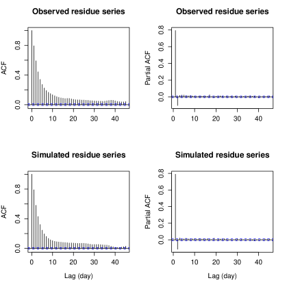
Figure 2: The sample ACF and PACF plots of the observed seasonality-removed daily average temperature series and simulated seasonality-removed daily average temperature series. The simulated seasonality-removed series have similar sample ACF and PACF as the observed seasonality-removed series.

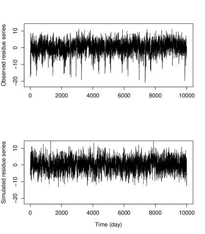
Figure 3: Time series plots of the observed seasonality-removed daily average temperature series and simulated seasonality-removed daily average temperature series. The magnitudes of variations in the observed seasonality-removed series do not match those in the simulated seasonality-removed series very well.

We now consider the prediction of bloom–dates. At the end of the current year, we generate 1000 series of the daily average temperatures of the whole next year using the fitted ARIMA model. For each crop, we then use (4) to obtain the probability of blooming on each successive day of the next year. This way we get a discrete predictive distribution for bloom–date of the new year.

Now suppose that we are at the end of the first day of the new year with its observed average daily temperature. We apply the fitted ARIMA model again to generate 1000 series of temperatures starting from the second day of the new year to the end of the year. We can then get another predictive distribution for the bloom–date of the new year. We repeat this procedure on each successive day, until the true bloom–date, at which time prediction ceases. If the true bloom–date of the new year were day 120 for example, we would get 120 successive predictive distributions. What we expect to see are increasingly more accurate predictions as the days progress toward the bloom–date and more and more information about the daily averages temperatures come to hand for that season. Growing confidence in that prediction would provide an increasingly strong basis for management decisions.

To see if our expectaions are realized, we perform a leave-one-out prediction procedure – at every step, for each crop, leave out one year of data for prediction assessment and use the remaining years for training the model. Let’s consider apple as an example. For each left-out year, we follow the above prediction scenario. We thus get 28 years (1937–1964) of assessments, with a total of 3643 predictive distributions. For each of these predictive distributions, we calculate the mean, median and mode as possible candidates for point predictions of the new bloom–date. Also, we calculate a quantile based 95% prediction interval (PI) for the new bloom–date. With all the 3643 predictive distributions, we can then estimate the root mean square error (RMSE) and the mean abosolute errors (MAE) of the point predictions, and the coverage probability and the average length of the 95% PI. The results are shown in Table 12.

Table 12: Cross validation results: The RMSEs and MAEs for point predictions using mode, median and mean are shown in column 2–7. The estimated coverages and average lengths of the 95% PIs are shown in the last two column respectively. The units for RMSE, MAE and average length of the 95% PI are day. The estimated coverage probabilities of these 95% PIs are generally too high.

	Mode		Median		Mean		95% PI
Crop	RMSE	MAE	RMSE	MAE	RMSE	MAE	Coverage	Ave. Len.
Apricot	6.74	5.12	6.58	5.06	6.62	5.14	0.99	33.24
Cherry	6.76	4.97	6.59	4.88	6.59	4.92	0.99	34.29
Peach	5.43	4.09	5.33	4.04	5.34	4.05	0.99	28.41
Prune	5.82	4.31	5.45	4.11	5.46	4.16	0.99	30.55
Pear	5.60	4.19	5.65	4.36	5.69	4.40	0.99	29.99
Apple	5.39	4.07	5.44	4.19	5.45	4.23	0.99	28.86

Table 13: Maximum, minimum and range of the observed bloom–dates for each crop in 1937–1964 in the Okanagan region

	Apricot	Cherry	Peach	Prune	Pear	Apple
Maximum (day)	126	136	135	138	139	146
Minimum (day)	94	102	105	111	110	115
Range (day)	32	34	30	27	29	31

We also provide in Table 13 the observed range of the bloom dates (the difference time between the maximal and minimal observed bloom dates) of each crop as a measure of natural variation of the bloom–dates for each crop. The mean, median and mode as point predictions perform roughly the same in terms RMSE and MAE. The RMSEs for all crops fall between 5.3 and 6.8 days, and the MAEs fall between 4.0 to 5.2 days. Considering the observed ranges of the bloom–dates, which vary from 27 to 34, our point predictions provide more useful information about the future bloom–dates. The estimated coverage probabilities of 95% PIs are too high for all crops, relative to the expected 95%. For each crop, the average length of the 95% PI is roughly the same as the observed range of the bloom–dates, in accord with the high estimated coverage probability. These imply that our 95% PIs incorporate too much uncertainty, possibly because that in the ARIMA model, we have included too much variability caused by periodic signals other than seasonal variation as the variability of the random noise.

We therefore reduce the variance of the white noise in the ARIMA model to half the estimated value, while keeping all the other estimated parameter unchanged. We use this new ARIMA model to generate daily average temperatures, and perform the above cross validation procedure again. The results (Table 14) show that while the accuracy of the point predictions is roughly the same as before, the estimated coverage probabilities and average lengths of the 95% PIs are reduced to reasonable values. This result does not confirm that the high estimated coverage probabilities are actually caused by the high uncertainty in the predicted daily average temperatures, but it at least adds weight to this explanation.

Table 14: Cross validation results when using variance reduced simulated daily average temperatures: The RMSEs and MAEs for point predictions using mode, median and mean are shown in column 2–7. The estimated coverages and average lengths of the 95% PIs are shown in the last two column respectively. The units for RMSE, MAE and average length of the 95% PI are day. The estimated coverage probabilities of these 95% PIs are reasonable.

	Mode		Median		Mean		95% PI
Crop	RMSE	MAE	RMSE	MAE	RMSE	MAE	Coverage	Ave. Len.
Apricot	6.91	5.20	6.78	5.12	6.72	5.08	0.94	24.87
Cherry	6.62	5.06	6.64	5.05	6.58	4.99	0.93	26.46
Peach	5.56	4.03	5.51	3.95	5.49	3.98	0.95	21.17
Prune	5.48	4.16	5.46	4.04	5.46	4.07	0.98	22.38
Pear	5.98	4.46	5.79	4.33	5.75	4.31	0.94	21.45
Apple	5.76	4.36	5.53	4.17	5.48	4.15	0.95	20.36

The above results for predictions derive from two models: Model AGDD for blooming event and the ARIMA model for daily average temperature. To check the performance of Model AGDD solely, we assume all the future daily average temperatures are known, and then perform the above leave-one-out procedure again. The results are reported in Table 15. Note that, in this case, since the uncertainty of the future daily average temperatures is totally eliminated, we can only get one predictive distribution for each test year. Therefore we cannot give a sensible estimate for the coverage probability of the 95% PIs. But we do see that the accuracies of these point predictions are much higher than those of our previous predictions, and the average lengths of the 95% PIs are much smaller. Although these are no longer real predictions, the results tend to validate our Model AGDD for blooming event. Also, this finding shows the importance of accurately modeling the covariate series and points to the need to improve the temperature forecasting models.

Table 15: Cross validation results if future daily average temperatures were known: The RMSEs and MAEs for point predictions using mode, median and mean are shown in column 2–7. The average lengths of the 95% PI are shown in the last column. The units for RMSE, MAE and average length of the 95% PI are day. The point predictions are very accurate, and the average lengths of the 95% PIs are short.

	Mode		Median		Mean		95% PI
Crop	RMSE	MAE	RMSE	MAE	RMSE	MAE	Average Length
Apricot	4.18	3.30	3.65	2.93	3.62	2.90	13.48
Cherry	3.74	2.93	3.39	2.43	3.46	2.42	18.43
Peach	3.43	2.85	3.35	2.78	3.27	2.76	12.67
Prune	3.06	2.54	2.98	2.50	2.93	2.36	11.46
Pear	2.93	2.11	2.64	1.89	2.67	2.00	9.21
Apple	2.12	1.86	2.04	1.71	1.97	1.61	8.29

4.6 More about predictive uncertainties

As noted above, we expected our point prediction to become more accurate and predictive uncertainty to become smaller as time approaches the true bloom date. To check this, for each crop, we calculate the MAE with median as point prediction and the average lengths of 95% PIs each day over the years of interest, starting from 90 days prior to the bloom–date (call it "lag -90") to 1 day prior to the bloom–date ("lag -1"). The results are shown in Figure 4 and 5 respectively. It is clear that for all crops, the MAE does become smaller and the average lenghth of 95% PIs becomes shorter as time approaches the true bloom–date. In fact, by the time we reach one month prior the bloom–date, the point prediction is quite accurate (the MAE is 3.5–5 days).

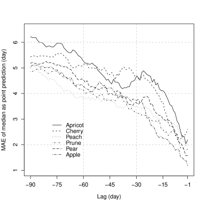
Figure 4: Change of the MAE of median with the change of lag. The point prediction becomes more accurate when time approaches the bloom date.

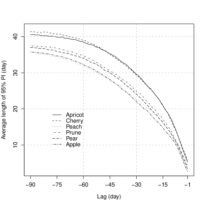
Figure 5: Change of the average length of 95% PIs with the change of lag. The predictive uncertainty decreases when time approaches the bloom date.

We now compare our predictor with two naive predictors: the first one being the 95% confidence interval (CI) of a normal fit to the observed data, i.e. $\pm 1.96$ standard deviation around the sample mean; the second one being an empirical quantile-based 95% CI of the observed data, i.e. 2.5%–97.5% sample quantiles. The length and percentage of the coverage of the normal fits are shown in Table 16. Although the length of the normal CIs are a few days shorter than our overall 95% PIs reported in Table 12, the coverages of the normal CIs are too low, especially for peach, prune and pear. Figure 6 shows that the histograms of the bloom dates of the crops are obviously skewed, which implies that the normal fit may not be a good choice. The length and coverage of the empirical quantile-based CIs are shown in Table 17. These CIs beat the Normal CIs in both length and coverage for most of the crops. However, the coverages of them are still lower than 95% except for Pear. The results reported in Table 12 for our predictor are calculated from the first day of a year to the actual bloom date, which have incorporated too much uncertainty. If we look at the predictions starting from one month prior to the bloom date to the actual bloom date, the results (Table 18) are much improved – the average lengths of the 95% PIs are much shorter and the estimated coverage probabilities now range from 95% to 98%. These results apparently are much better than those from both naive predictors.

Table 16: The length and the coverage of 95% CI of a normal fit to the observed bloom–dates for each crop in 1937–1964 in the Okanagan region

	Apricot	Cherry	Peach	Prune	Pear	Apple
Length	30.65	29.23	27.20	25.62	26.76	25.57
coverage	0.93	0.93	0.89	0.89	0.93	0.93

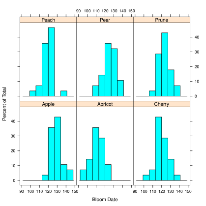
Figure 6: Histograms of the bloom dates of the corps. Most of the histograms are obviously skewed.

Table 17: The length and the coverage of the empirical quantile-based 95% CI of the observed bloom–dates for each crop in 1937–1964 in the Okanagan region

	Apricot	Cherry	Peach	Prune	Pear	Apple
Length	28.10	29.28	24.15	24.97	27.65	24.25
coverage	0.93	0.93	0.93	0.93	0.96	0.93

Table 18: The average length and the estimated coverage probability of 95% PIs of our predictions starting from one month prior to the bloom date to the actual bloom date

	Apricot	Cherry	Peach	Prune	Pear	Apple
Length	19.91	19.87	15.28	16.38	15.57	14.19
coverage	0.95	0.96	0.97	0.98	0.97	0.97

Another thing that interests us is the shape of the predictive distributions. To see this, we plot the predictive distribution of a “randomly” picked crop and test year – the predictive distribution of peach in year 1944 with daily average temperatures of the first 60 days of that year known (Figure 7). Note that the true bloom–date of peach in that year is day 125, and we have smoothed the discrete predictive distribution to a continuous curve. We see that the predictive distribution (the solid curve) is nearly bell-shaped which roughly looks like a normal distribution. Since this predictive distribution is calculated by plugging in the MLEs as if they were the true parameters, there is an uncertainty associated with this predictive distribution. Just as before, we use the bootstrap to assess this uncertainty – we calculate a quantile based 95% bootstrap confidence band (shown as the shaded area in Figure 7) for this predictive distribution. The plot shows that this confidence band is not too wide, so we basically can “trust” this predictive distribution.

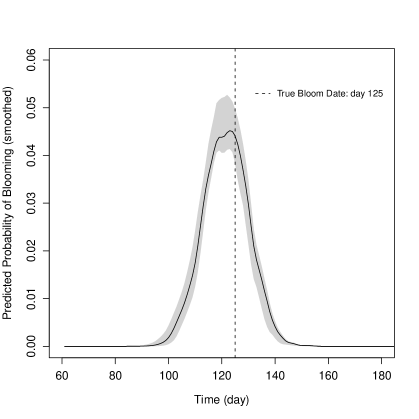
Figure 7: The predictive distribution (solid curve) of peach in year 1944 with daily average temperatures of the first 60 days of that year known. The shaded area is a 95% confidence band for this predictive distribution. The true bloom – date of peach in that year is day 125.

The validity of the bootstrap procedure arises again. Do the bootstrap estimates of the quantiles of the predictive probabilities reflect the true quantiles of the predictive probabilities? Again, we conduct a simulation study to answer this question. Take the same settings for the simulation as described in Section 4.3. For each sample size $S$, where $S\in\left\{30,\,80,\,150,\,400\right\}$, we now generate one more year of data as test data. For a fixed sample size $S$, for each sample, we estimate the model parameters, and we then use this set of of parameters to predict the bloom–date of the test year by assuming the first 60 days of temperatures are known. We then get 1000 predictive distributions for each sample size. For each future day, we take the 2.5% and 97.5% sample quantiles of the 1000 predictive probabilities to approximate a quantile based 95% confidence interval for the predictive probability. Now, randomly pick one sample, and then take 1000 bootstrap samples of this sample, and estimate model parameters using each bootstrap sample. With each set of estimated parameters obtained from the bootstrap, we can then make a prediction on the test year. With 1000 bootstrap samples, we get 1000 predictive distributions. For each future day, as with the simulated data, we can obtain a quantile based 95% bootstrap confidence interval for the predictive probability. We now compare the confidence intervals obtained in these two ways. Randomly picking one future day, the 95% confidence intervals for the predictive probability of blooming that day calculated using the simulated data and bootstrap are shown in Table 19. We can see that both types of confidence intervals become narrower when sample size becomes larger. For each sample size, the bootstrap interval is close to the interval obtained using the simulated data. Moreover, when the sample size reaches 400, the two types of intervals are basically identical. This result suggests that applying bootstrap might be a reasonable way to estimate the uncertainty of the predictive probabilities.

Table 19: Comparison of the 95% confidence intervals for predictive probabilities obtained using bootstrap and the simulated data.

	$S=30$	$S=80$	$S=150$	$S=400$
Bootstrap	(0.0300, 0.0350)	(0.0321, 0.0358)	(0.0300, 0.0320)	(0.0305, 0.0322)
Simulation	(0.0288, 0.0348)	(0.0298, 0.0332)	(0.0302, 0.0326)	(0.0307, 0.0320)

5 Conclusions

In this paper, we presented an application of our regression model for irreversible progressive events to a single phenological event – blooming event of six high-valued perennial crops. The approach we introduced here can be also widely applicable to the analysis of survival data and other similar time-to-event data.

For the blooming events of the six crops, our method provides a sensible way to estimate the important parameter $T_{base}$ in the definition of growing degree day (GDD) and our statistical analysis supports an earlier empirical finding – that the timing of a bloom event is related to AGDD, a cumulative unweighted sum of GDDs. Our method also provides useful point predictions of the future bloom–dates, as well as the assessment of the predictive uncertainties which is useful for risk analysts and policy makers. Our 95% PIs are excessively large however, quite probably because we have used a crude ARIMA model for predicting the future daily average temperatures. After reducing and then total eliminating the uncertainty about the daily average temperatures, we see increased accuracy of point predictions and much shortened 95% PIs. This observation validates our regression model for phenological events.

In our analysis, we did not consider the possible auto-correlation of the bloom date. In future, we will consider more complicated models to incorporate this. On the other hand, to improve estimation and prediction, we may build a multivariate model to encompass all crops as responses simultaneously. Moreover, if crops of multiple locations are involved, we will consider a spatial-temporal modeling approach for phenological events.

References

- Cai et al. (2010) Song Cai, James V. Zidek, and Nathaniel K. Newlands. Predicting sequences of progressive events times with time-dependent covariates. Technical report, Department of Statistics, The University of British Columbia, 333-6356 Agricultural Road, Vancouver, BC, V6T 1Z2, Canada, 2010.
- Chatfield (2004) Chris Chatfield. The Analysis of Time Series. Chapman & Hall / CRC, 6ed edition, 2004.
- Chuine (2000) Isabelle Chuine. A unified model for budburst of trees. Journal of Theoretical Biology, 207(3):337–347, December 2000.
- Cox and Hinkley (1979) D. R. Cox and D. V. Hinkley. Theoretical Statistics. Chapman & HallCRC, 1st edition, 1979.
- Efron and Tibshirani (1986) Bradley F. Efron and Robert J. Tibshirani. Bootstrap methods for standard errors, confidence intervals, and other measures of statistical accuracy. Statistical Science, 1(1):54–77, 1986.
- Efron and Tibshirani (1994) Bradley F. Efron and Robert J. Tibshirani. An Introduction to the Bootstrap. Chapman & HallCRC, 1st edition, 1994.
- Gienapp et al. (2005) Phillip Gienapp, Lia Hemerik, and Marcele Visser. A new statistical tool to predict phenology under climate change scenearios. Global Change Biology, 11:600–606, 2005.
- Kalbfleisch and Prentice (2002) John D. Kalbfleisch and Ross L. Prentice. The Statistical Analysis of Failure Time Data. Wiley-Interscience, 2nd edition, 2002.
- Murray et al. (1989) M. B. Murray, M. G. R. Cannell, and R. I. Smith. Date of budburst of fifteen tree species in britain following climatic warming. J. Appl. Ecol., 26:693–700, 1989.
- Wald (1949) Abraham Wald. Note on the consistency of the maximum likelihood estimate. Annal of Mathematical Statistics, 20:595–601, 1949.