Random Sequential Renormalization of Networks: Application to Critical Trees

Abstract

We introduce the concept of random sequential renormalization (RSR) for arbitrary networks. RSR is a graph renormalization procedure that locally aggregates nodes to produce a coarse grained network. It is analogous to the (quasi-)parallel renormalization schemes introduced by C. Song et al. [C. Song et.al., Nature (London) 433, 392 (2005)] and studied by F. Radicchi et al. [F. Radicchi et al., Phys. Rev. Lett. 101, 148701 (2008)], but much simpler and easier to implement. Here we apply RSR to critical trees and derive analytical results consistent with numerical simulations. Critical trees exhibit three regimes in their evolution under RSR. (i) For $N_{0}^{\nu}\lesssim N<N_{0}$, where $N$ is the number of nodes at some step in the renormalization and $N_{0}$ is the initial size of the tree, RSR is described by a mean-field theory, and fluctuations from one realization to another are small. The exponent $\nu=1/2$ is derived using random walk and other arguments. The degree distribution becomes broader under successive steps, reaching a power law $p_{k}\sim 1/k^{\gamma}$ with $\gamma=2$ and a variance that diverges as $N_{0}^{1/2}$ at the end of this regime. Both of these latter results are obtained from a scaling theory. (ii) For $N_{0}^{\nu_{\rm star}}\lesssim N\lesssim N_{0}^{1/2}$, with $\nu_{\rm star}\approx 1/4$ hubs develop, and fluctuations between different realizations of the RSR are large. Trees are short and fat with an average radius that is ${\cal O}(1)$. Crossover functions exhibiting finite-size scaling in the critical region $N\sim N_{0}^{1/2}\to\infty$ connect the behaviors in the first two regimes. (iii) For $N\lesssim N_{0}^{\nu_{\rm star}}$, star configurations appear with a central hub surrounded by many leaves. The distribution of stars is broadly distributed over this range. The scaling behaviors found under RSR are identified with a continuous transition in a process called “agglomerative percolation” (AP), with the coarse-grained nodes in RSR corresponding to clusters in AP that grow by simultaneously attaching to all their neighboring clusters.

I Introduction

Renormalization is a basic concept in statistical physics. It is a process whereby degrees of freedom in a system are successively eliminated by coarse graining. At the same time system parameters are rescaled to compensate for the decimation, and the smallest scale is reset to its original value amit . Since a series of such transformations is itself a transformation, the transformations $\{{\cal R}\}$ form a semi-group: the “renormalization group” (RG).

If the system is statistically invariant under $\{{\cal R}\}$, one speaks of RG invariance. An invariant system exhibits an asymptotic fixed point under the RG flow with scaling described by homogeneous functions. Prototypical RG fixed points are critical phenomena displayed at continuous phase transitions as for the Ising model, by a-thermal systems like directed Hinrich or ordinary Stauffer percolation, relativistic quantum field theories Zinn , or the Feigenbaum (period doubling) cascade in one-dimensional dynamical systems Feigenbaum . Systems with the same fixed point under RG are in the same universality class and share the same critical exponents.

It is natural to ask if similar concepts can be applied to glean meaningful information about complex networks. A positive answer was suggested in Ref. Song and has stirred much interest. In the present paper we start an investigation to further explore whether and in what sense this can be true.

For models on a lattice, coarse graining can be accomplished either in Fourier space or in real space. A typical real space RG proceeds heuristically by covering a spin lattice with a regular grid of boxes, and replacing the degrees of freedom in each box by a “super-spin” Stauffer . Interactions between spins in neighboring boxes are used to specify the couplings between super-spins.

However, many real world phenomena are better represented as complex networks rather than regular lattices. Although research in this area has exploded in recent years (for reviews see, e.g., Refs. newmanRev ; BA ; boccaletti ), our understanding of the statistical physics of complex networks has not caught up with the vast body of knowledge accrued over decades for lattice systems. Some phase transitions on networks (e.g., in the spreading of epidemics newman ; pastor ) are straightforward generalizations of critical phenomena on lattices. Yet it is not clear whether the RG, and real-space renormalization, in particular, can be applied systematically to complex networks.

Closely related to renormalization is the notion of fractal dimensions amit ; Zinn . Many complex networks are small world networks Milgram ; Watts , where the number of nodes within reach of any node via paths of length $r$ increases exponentially with $r$. Via any standard definition, this gives infinite fractal dimensions. However Song et al. Song , made claims to the contrary, finding finite fractal dimensions for several real-world networks based on a quasi-parallel renormalization scheme. A real-space RG for networks that is not based on the concept of fractal dimensions, but studied in terms of the flow under renormalization, was proposed by Radicchi et al. Radi1 ; Radi2 .

A fundamental issue pertinent to all the work up to now on renormalization of networks (see, for instance, Refs. Song ; Radi1 ; Radi2 ; Song2 ; Song3 ; Kim1 ; Kim2 ; Kim3 ) is that completely covering a network with equal size boxes leads to a number of unavoidable dilemmas that could lead to erroneous conclusions. Conceptually, covering the system with boxes of equal sizes is a flagrant violation of the original idea of Hausdorff Falconer , where the system ought to be covered with a partitioning whose elements have individually optimized sizes up to some largest size $r$. In most applications this is not a serious impediment, and a covering with equal size elements gives equivalent results. Thus most estimates of fractal dimensions in physics use fixed box sizes, although there are well known cases where this leads to erroneous results. The most famous one is given by any infinite but countable set of points, which according to Hausdorff, but not according to any covering algorithm with fixed box size, has zero dimension.

One reason why this problem can be neglected in many physical systems is that the number of points per box (or, more precisely, the weight of each box) has small fluctuations, in particular, relative to a distribution whose width increases exponentially with box size. For small world networks, where, indeed, the maximum number of nodes increases exponentially, the schemes of Refs. Song ; Song2 ; Song3 ; Kim1 ; Kim2 ; Kim3 may give misleading results because most boxes have only a few nodes. Then the problems associated with fixed box size become acute and there is no reason to believe that the results obtained are related to genuine fractal dimensions of the underlying graph.

Even with fixed box size, the covering should also be optimized with respect to the exact placement or tiling of the boxes, which is an NP hard problem Song3 . Heuristic methods for this optimization have been claimed to work Song ; Song2 ; Kim3 , but as a matter of fact they depend on the order in which boxes are laid down. Thus they are not true parallel substitutions of nodes by super-nodes, but quasi-parallel since the single step of tiling the whole network is implemented as a sequence of partial tilings. Combined with the problem of almost empty boxes, this means that the efficiency of the box covering algorithm changes both within each renormalization step (the boxes put down first contain in general more vertices than later boxes), and from one step to the next.

Another problem with the (quasi)parallel renormalization scheme is that each step of renormalization dramatically reduces the number of nodes in the network. Therefore few points and less statistics are obtained for analyzing renormalization flow. This becomes particularly serious in the case of small world networks which collapse to one node in a few steps, even when the initial network size is huge. This has been overcome to some extent in Ref. song10 by performing a renormalization where only parts of the network are coarse-grained at each step, at the cost of adding more parameters and making the results harder to interpret.

In view of these problems, we decided to study graph renormalization for unweighted, undirected networks by means of a purely sequential algorithm: At each step one node is selected at random, and all nodes within a fixed distance of it (including itself) are replaced by a single super-node. The super-node has links to all other nodes that were connected to the original subset absorbed into the super-node. This is repeated until the network collapses to a single node.

Our method avoids the problem of finding an optimum tiling as well as problems with almost empty boxes. A further advantage of our random sequential renormalization (RSR) procedure is that each step has a much smaller effect on the network, and thus the whole renormalization flow consists of many more single steps for a finite system and allows for a more fine grained analysis.

If there are fixed points underlying this RG flow, then they will manifest themselves in terms of (finite-size) scaling laws, which hold for large initial networks at intermediate times. Here time is measured by the number of steps in the RSR. At intermediate times, the system is far from both the initial network and the non-invariant final network composed of a single super node.

On any graph, including networks or lattices, the super-nodes can be viewed as clusters that grow by attaching to all of their neighboring clusters, up to a distance $b$ in the network of clusters. This process, called “agglomerative percolation”, has been solved exactly in one dimension and shown to exhibit scaling laws with exponents that depend on $b$ Son-2010 . On a square lattice in two dimensions, critical behavior is seen which is in a different universality class claire than ordinary percolation. Thus the scaling behavior seen in RSR occurs as a result of a type of percolation transition and is not restricted to cases where the underlying graph is fractal.

Here we apply our RSR methodology to critical trees and also find evidence for a critical point (which is, however, not a fixed point of the RSR!) where the number of links attached to any node (i.e., its degree) follows a power law and divergences appear for e.g. the variance of the degree distribution. The size of the networks at the transition point diverges as $N_{0}^{1/2}$, slower than the initial network size ($N_{0}$) in the limit of infinite system size. Below this transition, renormalized trees are short and fat with an average depth (or radius) which is ${\cal O}(1)$. We determine some critical exponents using random walk and other arguments, as well as a mean-field theory for the initial, uncorrelated phase. We use, in addition, the observation that all renormalized networks for $b=1$ eventually reach a star dominated by a central hub before they collapse to a single node. Our results are confirmed by means of finite-size scaling analyses of results from numerical simulations. These simulations also reveal scaling behavior for the probability distribution for the sizes of networks that first reach a star configuration. This turns out to be equivalent to the distribution of sizes one step before the network collapses to a single node. Stars first appear for renormalized networks when the size of the network is $N\lesssim N_{0}^{\nu_{\rm star}}$ with $\nu_{\rm star}\approx 1/4$.

In Sec. II, we define the general RSR procedure for any network as well as the specific ensemble of networks we analyze in this paper. Section III presents our theoretical and numerical results for RSR of critical trees. Finally, we end with conclusions and outlook for future work in Sec. IV.

II The Model

II.1 Random Sequential Renormalization

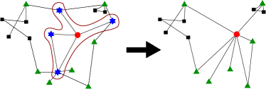
Figure 1: (Color online) One step of RSR with $b=1$. The randomly chosen target node (red circle), absorbs all its nearest neighbors (blue stars). All links to the absorbed nodes (from green triangular nodes) are then redirected to the target. Alternatively one can view the super-node as a cluster (bounded by the red curve) that subsequently grows by invading its neighboring clusters.

For any undirected, unweighted graph, RSR with radius $b$ ($b=1,2,\ldots$) is defined as follows: Starting with a graph with $N_{0}$ nodes, we produce a sequence of graphs of strictly decreasing sizes $N_{t}$ with $0<t\leq T$ and $N_{T}=1$. For each step $t\to t+1$ ($t$ is called “time” in the following):
(i) We choose randomly a target node $i\in[1,\ldots,N_{t}]$.
(ii) We delete all nodes that can be reached from $i$ by at least one path of length $1\leq\ell\leq b$.
(iii) We also delete all links between these chosen nodes, and all links connecting them to $i$.
(iv) Each link connecting any node outside this neighborhood to a deleted node is redirected towards the target. (v) If this creates a multiple link between any two nodes, it is replaced by a single link.

Hence the target node $i$ is replaced by a super-node that maintains all links to the outside. Its internal features, however, are erased from the network, consistent with coarse graining. Figure 1 shows an example of one step of RSR for $b=1$. After absorbing its neighbors the super-node is treated like any other node and the process repeats until the network collapses into a single node. One could also vary the probability of choosing a target node by a function of its mass (the number of nodes absorbed into it), or its degree (the number of links attached to it), but these aspects are not explored here.

When $b=1$, only nearest neighbors of the target node are deleted. For $b>1$ each step can be implemented by performing $b$ successive decimations with radius one on the same target. Although this method is slightly slower than an optimal coding where all nodes within distance $\leq b$ of the target are found and deleted in a single step, it reduces code complexity and potential sources of errors.

For any radius $b\geq 1$, RSR exhibits two trivial fixed points: a graph consisting of a single node, and an infinitely long chain. For a long but finite chain, the time until a single node is reached is $T=\lceil N_{0}/2b\rceil$. In one dimension, the exact probability to find any consecutive sequence of node masses for any $N_{0}$ and at any time has been determined Son-2010 . At late times, and for large $N_{0}$ the mass distribution of the nodes exhibits scaling both at small and large sizes with (different) exponents that depend on $b$. For $b=1$ another fixed point exists, which is a star with infinitely many leaves. In that limit, the probability to choose the central hub of the star as the target vanishes. With probability one, a single leaf is removed during each RSR step. For a finite number $N_{\rm star}-1$ of leaves, a star has an average life time $\bar{T}={\cal O}(N_{\rm star})$ before it collapses into a single node. Notice that simple stars are not fixed points for $b>1$, as any star reduces to a single node in one step with probability one. In this paper we study only the case of RSR with $b=1$.

II.2 Initial graph ensemble

The ensemble of critical trees is generated as follows: Starting with a single node, each node can have 0, 1, or 2 offspring with probabilities $1/4$, $1/2$ and $1/4$. (Hence the mean number of offspring is 1.) The process runs until it dies due to fluctuations. The sizes of trees obtained in this way are distributed according to an inverse power law $P(N_{0})\sim N_{0}^{-3/2}$ Stauffer . From these we pick a large ($\approx 10^{2}-10^{3}$) ensemble of trees with the desired (large) $N_{0}(\pm 10\%)$, and discard all others. Note that simply truncating trees that survive up to $N_{0}$ would give a biased sampling of the ensemble.

This construction generates a rooted tree, with important consequences for joint degree distributions of adjacent nodes. The direction of growth leaves its imprint on them. For ordinary undirected random graphs (Erdös-Renyi graphs), it is well known that the degree distribution for pairs of nodes obtained by randomly choosing a link is different from that obtained by choosing any two nodes at random. If the degree distribution is $p_{k}$, the distribution of degree pairs for linked nodes is not $p_{k}p_{k^{\prime}}$, but $kk^{\prime}p_{k}p_{k^{\prime}}/\langle k\rangle^{2}$, because higher degree nodes have a greater chance of being attached to a randomly chosen link. For the present model, two connected nodes are always in a mother - daughter relationship. In particular, all nodes have in-degree one; that is, they have one mother (except for the root). If $k$ is the out-degree of the mother and $k^{\prime}$ the out-degree of the daughter, then the distribution of degree pairs obtained by randomly choosing links is

$${kp_{k}p_{k^{\prime}}\over\sum_{l,l^{\prime}}lp_{l}p_{l^{\prime}}}={kp_{k}p_{k^{\prime}}\over\langle k\rangle}\quad.$$ (1)

While high degree mothers have a greater chance of appearing in a pair than low degree mothers, no such bias holds for daughters. Otherwise said, if we pick a random node, the out-degrees of its daughters will be distributed according to $p_{k^{\prime}}$, while the out-degree of its mother is distributed $\propto kp_{k}$. Notice that this implies that our ensemble of critical trees is not equivalent to the ensemble of critical Erdös-Renyi graphs.

In the following, we shall always denote by $p_{k}$ the distribution of out-degrees, and we will, for simplicity, always call $k$ the “degree” (even though the real degree is $k+1$).

III Analytical Calculations and Simulation Results

III.1 Evolution of the tree size, $N$

Let $n_{k}$ be the number of nodes with degree $k$, and $N=\Sigma_{k}n_{k}$ the total number of nodes in the tree (i.e., its size, at a given step). Both $N$ and $n_{k}$ are fluctuating functions of time $t$. Since target nodes are picked randomly, the average degree of the target is $\langle k\rangle\equiv N^{-1}\Sigma_{k}kn_{k}=1-1/N$, where the last equality follows from the fact that the total number of links in a tree is always $N-1$. Since all the target’s neighbors (both its mother, unless it is the root, and any daughters) are deleted in the subsequent renormalization step, we get the exact result

$$\overline{\frac{\Delta N}{\Delta t}}=-\langle k\rangle-1+{1\over N}=-2+{2\over N}\quad.$$ (2)

Here the overline denotes an average over the randomness of the last step only, while brackets denote ensemble averages (except for $\langle k\rangle$) including also the randomness from previous RSR steps. Approximating $t$ by a continuous variable and performing such an ensemble average gives

$$\langle N\rangle=N_{0}-2t+\ln\left({N_{0}-1\over\langle N\rangle-1}\right)\;.$$ (3)

(The integration can only be performed for $N>1$.) We have replaced $\langle 1/N\rangle$ on the right hand side of Eq. (3) by $1/\langle N\rangle$, which is a mean-field approximation. We show in Sec. III.5 that this mean-field regime extends up to a time when $N\sim{\cal O}(N_{0}^{1/2})$.

III.2 Evolution of the degree distribution

The probability that a randomly chosen node in a network has degree $k$ is $p_{k}=n_{k}/N$. The change of $n_{k}$ in one step of renormalization has three contributions,

$$\overline{\frac{\Delta n_{k}}{\Delta t}}=r_{k}+s_{k}+q_{k},$$ (4)

where:

• $r_{k}$ is a loss term associated with the possibility that the target had (old) degree $k$ before the considered renormalization step. It is

  $$r_{k}=-p_{k}\quad.$$ (5)

• $s_{k}$ is a loss term from the (old) neighbors of the target having degree $k$. Assuming no degree correlations, which is also a mean-field approximation, and summing over all (old) degrees $k^{\prime}$ of the target gives

  $$s_{k} = -\sum_{k^{\prime}}k^{\prime}p_{k^{\prime}}p_{k}-\sum_{k^{\prime}}p_{k^{\prime}}\Biggl{(}{kp_{k}\over\sum_{l}lp_{l}}\Biggr{)}$$ (6)

  $$= -\langle k\rangle p_{k}-{kp_{k}\over\langle k\rangle}$$

  $$\approx -(1+k)p_{k}\quad.$$

  Here the first term is the contribution of the daughters, while the second is due to the mother. This assumes that the target is not the root. For simplicity we shall neglect that possibility in the following, which makes errors of ${\cal O}(1/N)$. These are negligible for large $N$. The last line follows from $\langle k\rangle=1-1/N\approx 1$, which is a good approximation for the same reason.

• $q_{k}$ is a gain term arising from the possibility that the target acquires new degree $k$. Assume that the old degree of the target was $m$, that the degrees of its daughters were $k_{1},\ldots,k_{m}$, and that the degree of its mother was $k_{0}$ — and that all degrees are uncorrelated. Then

  $$q_{k}=\sum_{m}p_{m}\sum_{k_{0}\ldots k_{m}}{k_{0}p_{k_{0}}\over\langle k\rangle}\;\prod_{i=1}^{m}p_{k_{i}}\;\;\delta_{k_{0}+\ldots k_{m}-1,k}\;.$$ (7)

  This term is not very transparent. For a more tractable formulation we use the generating function methods discussed next.

III.3 Generating Functions

The generating function for $p_{k}$ is

$$G(x)=\sum_{k}p_{k}x^{k}\quad,$$ (8)

and moments of the distribution are given by

$$\langle k^{m}\rangle=\left[\left(x\frac{d}{dx}\right)^{m}G(x)\right]_{x=1}\quad.$$ (9)

Similarly, the generating function for the gain term is

$$Q(x)=\sum_{k}q_{k}x^{k}\quad.$$ (10)

If a variable has a given generating function, then the generating function for the sum of that variable over $m$ independent realizations is given by the $m^{th}$ power of that generating function newman01 . Hence, if the target node has degree $m$, the generating function for the sum of degrees of all its daughters is $[G(x)]^{m}$. Using the above definitions and $G^{\prime}(1)=\langle k\rangle\approx 1$, we get

$$Q(x)=\sum_{m}p_{m}G^{\prime}(x)G^{m}(x)=G^{\prime}(x)G(G(x))\;.$$ (11)

This, together with Eqs. (2) through (6), leads to

$$\overline{\frac{\Delta G(x)}{\Delta t}}={1\over N}[G^{\prime}(x)G(G(x))-xG^{\prime}(x)]+{\cal O}(1/N^{2})\;\;.$$ (12)

A more tedious calculation, which requires generating functions for the root of the tree – arrives at the neglected ${\cal O}(1/N^{2})$ terms. The exact result (assuming no correlations) is

$$\overline{\frac{\Delta G(x)}{\Delta t}} = {1\over N}[G^{\prime}(x)G(G(x))-xG^{\prime}(x)]$$ (13)

$$+ {1\over N^{2}}[G(G(x))-G(x)]\quad.$$

One checks easily that this satisfies the conditions that $G(1)$ is constant and $G^{\prime}(1)=1-1/N$ for all $t$.

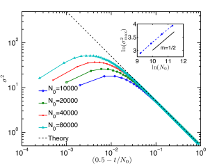
Figure 2: (Color online) Comparison between the variance of the degree distribution obtained from Eq. (16) and simulations for different system sizes, $N_{0}$. The mean-field theory extends over a larger range for increasing $N_{0}$. The inset shows that the maximum variance in RSR observed numerically scales as $N_{0}^{1/2}$, in agreement with our scaling ansatz Eq. (17).

III.4 Variance of the degree distribution

Obtaining the time evolution of the variance of the degree distribution requires an expression for the time evolution of the second derivative of $G$. From Eq. (12) it follows that

$$\overline{\frac{\Delta G^{\prime\prime}(1)}{\Delta t}}={2G^{\prime\prime}(1)\over N}+{\cal O}(1/N^{2})\;\;.$$ (14)

Making the same steps and approximations as in subsection III.1 gives

$${dG^{\prime\prime}(x)\over dt} = {d\langle k^{2}-k\rangle\over dt}$$ (15)

$$= {\frac{2\langle k^{2}-k\rangle}{\langle N\rangle}}+{\cal O}(1/\langle N\rangle^{2})$$

$$\approx {2\langle k^{2}-k\rangle\over N_{0}-2t}\;.$$

Integrating, fixing the integration constant by the condition $\langle k^{2}\rangle_{0}=3/2+{\cal O}(1/N_{0})$, and rewriting the result in terms of the variance of the degree distribution $\sigma^{2}$ gives

$$\sigma^{2}\equiv\langle k^{2}\rangle-\langle k\rangle^{2}\approx{N_{0}\over 2(N_{0}-2t)}\approx{N_{0}\over 2N}\quad.$$ (16)

In Fig. 2 we compare Eq. (16) for the variance of the degree distribution with numerical simulations of RSR for different initial sizes of critical trees. We see perfect agreement at early times, but increasingly larger disagreement at later times. This is only in part due to the neglected higher order terms in $1/N$. Another source of error at late times is that $N$ exhibits large fluctuations compared to its average. Also, degree correlations develop. Hence, the mean-field approximation breaks down for large $t$. But we also see from Fig. 2 that agreement between theory and numerical results extends over a broader range for increasing system size $N_{0}$.

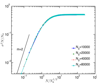
Figure 3: (Color online) Scaling of the variance of the degree distribution obtained from RSR. The data are the same as in Fig. 2, but the axes are different. They are chosen according to the scaling ansatz Eq. (17), and give excellent data collapse. The straight line has slope $m=2$.

To understand better the behavior at late times (small $N/N_{0}$), we replot the same data using a finite-size scaling (FSS) method in Fig. 3. This plot demonstrates that the scaling ansatz

$$\sigma^{2}=\frac{N_{0}}{N}g\Bigl{(}\frac{N}{N_{0}^{\nu}}\Bigr{)}\quad,$$ (17)

with scaling exponent $\nu=1/2$ gives excellent data collapse. We derive the result $\nu=1/2$ in the next subsection. The scaling function $g(x)$ satisfies $g(x)\to 1/2$ for $x\to\infty$, in agreement with Eq. (16). In addition, the network must, by definition, end up as a star before it collapses. Assuming that the star consists of a central hub surrounded by low degree nodes (which is verified numerically), its variance will scale with its size as $\sigma^{2}\sim N$. Also, the variance of the degree distribution of the star must be independent of the initial size $N_{0}$. These considerations lead to the conclusion that $g(x)\to x^{2}$ as $x\to 0$. Finally, in the scaling ansatz, $g$ and its derivative are continuous functions. As a result the maximum variance occurs when $N\sim N_{0}^{1/2}$ so that the maximum value of $\sigma^{2}\sim N_{0}^{1/2}$, in agreement with the inset of Fig. 2. Scaling laws like Eq. (17) in terms of homogeneous functions are well known from critical phenomena amit ; Zinn , where they describe finite-size scaling with several control parameters such as temperature and magnetic field.

III.5 Fluctuations of the system size and the relaxation time

In this subsection we derive the result $\nu=1/2$ by considering fluctuations around the average value of $\Delta N/\Delta t$, and the resulting fluctuations both of $N_{t}$ and of the relaxation time $T$. (Recall that the latter is defined as the time when the tree is first reduced to a single node.) Here we explicitly label the fluctuating number of nodes with its time dependence $N_{t}$.

Generalizing Eq. (2) and neglecting the ${\cal O}(1/N)$ term, we make the ansatz

$${\Delta N_{t}\over\Delta t}=-2+\epsilon_{t}\quad.$$ (18)

Here $\epsilon$ is a random variable with zero mean and with variance equal to the variance of the degree distribution $\sigma^{2}_{t}$, which, on average, increases with time $t$. Assuming no degree correlations, the random variables $\epsilon_{t}$ at different times are also uncorrelated, and

$$\langle\epsilon_{t}\epsilon_{t^{\prime}}\rangle=\delta_{t,t^{\prime}}\sigma^{2}_{t}\;.$$ (19)

Thus the fluctuations of $N_{t}$ are given by

$$\delta N_{t}\equiv N_{t}-\langle N_{t}\rangle=\sum_{t^{\prime}=0}^{t-1}\epsilon_{t^{\prime}}.$$ (20)

Since $\sigma_{t}$ is finite for all $t$, the central limit theorem implies that $\delta N_{t}$ is Gaussian for large $t$ with variance

$${\rm Var}[\delta N_{t}] = \sum_{t^{\prime}=0}^{t-1}\sigma^{2}_{t^{\prime}}\approx\sum_{t^{\prime}=0}^{t-1}{N_{0}\over 2(N_{0}-2t^{\prime})}$$ (21)

$$\approx {N_{0}\over 4}\ln{N_{0}\over\langle N_{t}\rangle}\;.$$

This estimate has to break down when typical fluctuations of $N_{t}$ are as big as its average, or when ${\rm Var}[\delta N_{t}]\approx\langle N_{t}\rangle^{2}$. We claim that this happens at a time when $\langle N_{t}\rangle\sim N_{0}^{1/2}$, explaining the fact that $\nu=1/2$. Indeed, when $\langle N_{t}\rangle\sim N_{0}^{\nu}$ with some positive exponent $\nu$, then ${\rm Var}[\delta N_{t}]\sim N_{0}\ln N_{0}>N_{0}$ for large $N_{0}$, implying that it is larger than $\langle N_{t}\rangle^{2}$ for any $\nu<1/2$. On the other hand, ${\rm Var}[\delta N_{t}]$ increases less quickly than $\langle N_{t}\rangle^{2}$ for any $\nu>1/2$, showing that the initial scaling regime breaks down when $\langle N_{t}\rangle\sim N_{0}^{\nu}$ with $\nu=1/2$.

Fluctuations of the relaxation time $T$ are obtained by demanding that $N_{T}=1$, which gives

$$2T-\sum_{t^{\prime}=0}^{T-1}\epsilon_{t^{\prime}}=N_{0}\;.$$ (22)

Hence, for large $N_{0}$, $T$ is distributed as an inverse Gaussian variate which is well approximated in the large $N_{0}$ limit by an ordinary Gaussian. Strictly, its variance cannot be calculated exactly, since the summation extends beyond the limit of applicability of our theory. To take this into account, we first convert the summation over $t^{\prime}$ to an integral over $N$ and truncate the integral at $N_{0}^{1/2}$, where the mean-field theory breaks down. Integration gives

$${\rm Var}[\delta T]={1\over 32}N_{0}\ln N_{0}\;$$ (23)

plus lower order terms. This is compared with the simulation results shown in the inset of Fig. 4, finding good agreement.

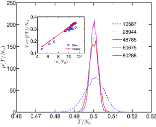
Figure 4: (Color online) Distributions of relaxation times for various values of $N_{0}$. The inset compares the variance of these distributions to Eq. (23) finding good agreement.

III.6 Scaling of maximum degree

A simple way to track the formation of hubs under RSR is to measure the maximum degree in the network $k_{\rm max}$. A naive scaling assumption is that when a few large hubs together with many low degree nodes dominate, $\sigma^{2}\sim k_{\rm max}^{2}/N$. Using Eq. (17) gives

$$k_{\rm max}\sim N_{0}^{1/2}f\left(\frac{N}{N_{0}^{1/2}}\right)\quad\;.$$ (24)

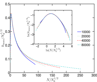
Figure 5: (Color online) FSS analysis of $k_{\rm max}$ using Eq. (24). There is perfect data collapse in the region $N\sim N_{0}^{1/2}$.

Figure 5 compares this equation to results from numerical simulations. While there are clear (and expected) deviations for $N/N_{0}^{1/2}\to\infty$, the collapse in the intermediate region $N\sim N_{0}^{1/2}$, where $\sigma^{2}$ achieves its maximum, is perfect. As before, assuming that the tree evolves to a star with a hub at its center suggests that $f(x)\sim x$ as $x\to 0$. However in Fig. 5 we do not observe this behavior as the fitting region is small and there is still some curvature in the scaling function. As for $\sigma^{2}$, our theory predicts that the largest value of $k_{\rm max}$ observed under RSR scales as $N_{0}^{1/2}$ and agrees with the data seen in the inset of Fig. 5.

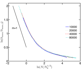
Figure 6: (Color online) FSS analysis of $k_{\rm max}/k_{\rm max,2}$. This ratio increases as one large hub separates from the rest of the degree distribution. The data show good agreement with the scaling ansatz Eq. (25). The line with slope $-1$ indicates the theoretical prediction as the network approaches a star.

III.7 Ratio of the largest degree to the second largest degree

The ratio of $k_{\rm max}$ to the second largest degree $k_{{\rm max},2}$ (provided that $k_{{\rm max},2}>0$) is shown in Fig. 6. It agrees with an FSS analysis using the same exponent $\nu=1/2$,

$${k_{\rm max}\over k_{{\rm max},2}}=h\left(\frac{N}{N_{0}^{1/2}}\right)\quad.$$ (25)

Once again the extreme limits of the scaling function $h$ can be determined. For the initial network the largest and second largest degree are equal, so $h(x\to\infty)\to 1$. For a pure star of size $N$, $k_{\rm max}/k_{{\rm max},2}=N$. As shown in Section III.10, stars first appear when $N\sim N_{0}^{\nu_{\rm star}}$ with $\nu_{\rm star}\approx 1/4$. In that case $k_{\rm max}/k_{{\rm max},2}\sim N_{0}^{1/4}$. Hence $h(N_{0}^{-1/4})\sim N_{0}^{1/4}$, or $h(x\to 0)\sim 1/x$. Figure 6 shows that $h$ is increasing in this limit, although the asymptotic regime is not yet reached for the system sizes studied.

III.8 Degree distribution

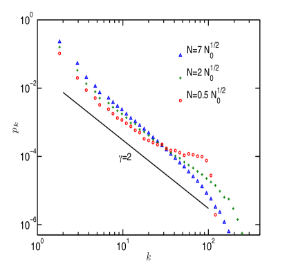
Figure 7: (Color online) Log-log plot of the degree distribution $p_{k}$ for trees with $N_{0}=8\times 10^{4}$ at three values of $N$: $N=7N_{0}^{1/2}$, $N=2N_{0}^{1/2}$ and $N=0.5N_{0}^{1/2}$. These distributions are obtained by averaging over different initial networks and different realizations of RSR. The distribution widens and then becomes more narrow on decreasing $N$ as hubs separate from the rest of the nodes during the transition. The data are consistent with our theoretical prediction that at the critical point $p_{k}\sim k^{-\gamma}$ with $\gamma=2$.

Degree distributions for large initial trees at three points in the evolution are shown in Fig. 7. Critical trees start with a narrow degree distribution, which becomes broader and broader under RSR. The degree distribution gradually transforms into a power law distribution as $N$ approaches $\sim N_{0}^{1/2}$. For a power law degree distribution $p(k)\sim k^{-\gamma}$, the variance obeys

$$\sigma^{2}\sim\int^{k_{\rm max}}k^{2-\gamma}dk\sim k_{\rm max}^{3-\gamma}\quad.$$ (26)

From the scaling result at the transition, $\sigma^{2}\sim k_{\rm max}\sim N_{0}^{1/2}$, we get $\gamma=2$, consistent with the data shown.

With the formation of a giant hub at the transition, a bump appears at large $k$ in $p_{k}$. This is clearly visible for $N=0.5N_{0}^{1/2}$ in Fig. 7. Note that the distributions shown in this figure are obtained by averaging over many initial networks and many realizations of RSR. In the degree distribution of a single network a gap emerges between the largest hub and the rest of the nodes, for $N\sim N_{0}^{1/2}$ as demonstrated in Fig. 6.

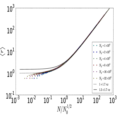
Figure 8: (Color online) Mean radius $r$ of trees as a function of $N/N_{0}^{1/2}$. Agreement with Eq. 32 is excellent with $\alpha=1.7$ as indicated. Fluctuations cannot be ignored for small $N/N_{0}^{1/2}$ when mean-field theory breaks down and the bounds are no longer valid.

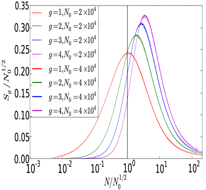
Figure 9: (Color online) The evolution of the number of nodes in the first four shells as a function of $N/N_{0}^{1/2}$ for two different system sizes. Note that $S_{1}$ crosses $S_{2}$ to become the largest shell at $N=N_{0}^{1/2}$. The other shells vanish increasingly faster as $N$ decreases further.

III.9 Mean-field theory for average radius of trees

The sum of the distances of nodes from the root in a tree of size $N$ can be written as

$$R=\sum_{x=1}^{N-1}g_{x}\quad,$$ (27)

where $g_{x}$ is the distance of node $x$ from the root. It is simplest to consider that (except for the root) the mother of a target node absorbs her (target) daughter plus all of that daughter’s daughters. Consider node $x$ at distance $g_{x}>1$. If the root is the target in the next RSR step, $g_{x}$ is reduced by $1$. If an ancestor of $x^{\prime}s$ mother is hit, which is not the root, then $g_{x}$ is reduced by $2$. If either $x$ or her mother is the target, then $x$ disappears, contributing zero to $R$. Hence the position of $x$ evolves in the continuous time approximation on average as

$$N{\partial g_{x}\over\partial t}=-1-2(g_{x}-2)-2g_{x}=-4g_{x}+3\quad,$$ (28)

for $x>1$. For $x=1$

$$N{\partial g_{x}\over\partial t}=-2\quad.$$ (29)

We can write the evolution in terms of the average number of nodes instead of time. As before, in mean-field we ignore fluctuations in $N$ about its average $\langle N\rangle$, in $R$ about its average $\langle R\rangle$, and in the number of nodes at distance $1$ in the tree $S_{1}$ about its average $\langle S_{1}\rangle$. This gives, after dropping all angular brackets,

$${dR\over dN}={2R\over N}-{3\over 2}(1-{1\over N})+{S_{1}\over 2N}\quad.$$ (30)

Defining the average radius $r=R/N$ with initial value $r_{0}=\alpha N_{0}^{1/2}$ for large $N_{0}$, the constant $\alpha\sim{\cal O}(1)$ depends on the precise rule for constructing critical trees. Equation (30) can be solved to get

$$r(N)={3\over 2}\Bigl{(}1-{N\over N_{0}}\Bigr{)}+\alpha{N\over N_{0}^{1/2}}-{N\over 2}\int_{N}^{N_{0}}dy\Bigl{(}{S_{1}\over y^{3}}\Bigr{)}\;.$$ (31)

Bounds on $r(N)$ can be placed based on the fact that $1\leq S_{1}<N$ to get

$$1+\alpha\Bigl{(}{N\over N_{0}^{1/2}}\Bigr{)}-{N\over 2N_{0}}<r\leq$$

$${3\over 2}\Bigl{(}1-{N\over N_{0}}\Bigr{)}+\alpha\Bigl{(}{N\over N_{0}^{1/2}}\Bigr{)}-{1\over 4N}+{N\over 4N_{0}^{2}}\quad.$$ (32)

These bounds are tested against numerical data in Fig. 8 showing excellent agreement, up until the regime where $N$ becomes small compared to $N_{0}^{1/2}$. At that point mean-field theory breaks down. As the trees start to exit the mean-field regime, their average radius becomes order unity even for $N\sim N_{0}^{1/2}\to\infty$. Figure 9 shows the evolution of the average number of nodes at distances 1, 2, 3, and 4 from the root, ($S_{1},\;S_{2},\;S_{3},\;{\rm and}\;S_{4}$, respectively). At $N=N_{0}^{1/2}$, $S_{1}$ becomes the largest shell, and $S_{2}$ seems to be exactly equal to $S_{1}$ at that point. All other shells vanish compared to $S_{1}$ for smaller $N$. This is the origin of the finite radius of renormalized trees near the end of the mean-field regime.

III.10 Distribution of last sizes and the star regime

Before the network reaches the trivial fixed point at $N=1$ it must first turn into a star. The star eventually collapses into a single node when the central node is hit as the target.

We define the quantity $N_{\ell}$ to be the size of the network one step before it dies. Figure 10 shows an FSS plot for the probability distribution of $N_{\ell}$. More precisely, it shows $N_{\ell}^{1.4}\;p(N_{\ell})$ against $N_{\ell}/N_{0}^{1/4}$. The data collapse seen suggests a scaling form

$$p(N_{\ell})\sim\frac{1}{N_{\ell}^{\tau}}\Phi(N_{\ell}/N_{0}^{D}),$$ (33)

with $\tau=1.4\pm 0.1$, $D=0.25\pm 0.05$. The scaling function $\Phi(x)$ seems to approach a constant for $x\to 0$, suggesting that $p(N_{\ell})$ tends to a power law, $p(N_{\ell})\sim N_{\ell}^{-\tau}$, for $N_{\ell}\ll N_{0}^{1/4}$.

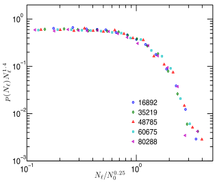
Figure 10: (Color online) FSS analysis for the distribution of last sizes based on Eqs. (33)-(36) with $\tau=1.4\pm 0.1$ and $D=0.25\pm 0.07$. In view of the comment after Eq. (34), $p(N_{\ell})$ is replaced with $p(N_{\ell})/2$ for $N_{\ell}=2$.

From the distribution of $N_{\ell}$ we can determine the distribution of sizes when the tree first turns into a star. Let us call $s$ the size when the renormalized tree first reaches a star configuration, and $p_{s}(s)$ its distribution. In each subsequent time step the star can either shrink by exactly one node (probability $1-1/N$), or it can be reduced immediately to a single node (probability $1/N$). Starting with a star of size $s$, the conditional probability to end up at final size $N_{\ell}$ is

$$p(N_{\ell}|s)=\left\{\begin{array}[]{l c c}{\displaystyle{1\over s}}&,&N_{\ell}=s\\ \\ \displaystyle\prod_{t=1}^{s-N_{\ell}}\frac{s-t}{s-t+1}\frac{1}{N_{\ell}}=\frac{1}{s}&,&2<N_{\ell}<s\\ \\ {\displaystyle{2\over s}}&,&N_{\ell}=2\end{array}\right.$$ (34)

where the last line comes from the degeneracy of a star with two nodes and is required for proper normalization. Assuming that $p_{s}(s)$ has a scaling form with possibly new exponents and a new scaling function $\phi$,

$$p_{s}(s)\sim\frac{1}{s^{\alpha}}\phi(s/N_{0}^{\beta})\;,$$ (35)

we obtain

$$p(N_{\ell}) = \sum_{s\geq N_{\ell}}p(N_{\ell}|s)p_{s}(s)$$ (36)

$$\approx \int_{N_{\ell}}^{\infty}ds{\phi(s/N_{0}^{\beta})\over s^{1+\alpha}}$$

$$= {1\over N_{\ell}^{\alpha}}\Psi(N_{\ell}/N_{0}^{\beta})$$

with $\Psi(x)=x^{\alpha}\int_{x}^{\infty}dx^{\prime}\;\phi(x^{\prime})/x^{\prime 1+\alpha}$. This agrees with Eq. (33), if we identify $\alpha=\tau$, $\beta=D$, and $\Psi(x)=\Phi(x)$. Thus the distributions of $s$ and of $N_{\ell}$ have the same exponents, if they obey FSS, which we verified numerically.

IV Conclusion

To study invariant properties of graphs under coarse graining, we have introduced the random sequential renormalization (RSR) method, where in each step only a part of the network within a fixed distance $b$ from a randomly chosen node collapses into one node. RSR is easy to implement and eliminates the problem of finding an optimum tiling of the network. In addition, the small effect of each decimation gives a much more detailed statistical picture of the renormalization flow. We applied the RSR with $b=1$ to critical trees and derived results analytically, finding good agreement with numerical simulations.

Under renormalization a critical regime appears when the size of the tree $N\sim N_{0}^{\nu}$ with $\nu=1/2$. The behavior of the tree before this regime is reached is described using a mean-field theory based on generating functions. There is a constant $c\simeq 1$ such that the degree distribution of the network is scale free, $p_{k}\sim k^{-\gamma}$ with $\gamma=2$, in the limit $N_{0}\to\infty$ and $N/N_{0}^{1/2}=c$. Both the variance of the degree distribution $\sigma^{2}$ and the maximum degree in the network $k_{\rm max}$ diverge as $N_{0}^{1/2}$ in this limit. Both of these quantities are described by crossover functions exhibiting finite-size scaling that connect the mean-field regime to a regime for $N_{0}^{1/4}\lesssim N\lesssim N_{0}^{1/2}$ when hubs start to emerge. Results from numerical simulations agree with a scaling theory we develop to describe this fixed point. Trees are short and fat near this point with an average depth ${\cal O}(1)$. As RSR proceeds further, star configurations start to appear for $N\sim N_{0}^{\nu_{\rm star}}$ with $\nu_{\rm star}\approx 1/4$. The distribution of star sizes seems to obey FSS, characterized by its own critical exponents, which we were not able to derive analytically.

We began this investigation to study in a more controlled way claims made in the literature about real-space renormalization of complex networks Song ; Radi1 ; Radi2 . In the most detailed previous study Radi1 ; Radi2 many of the findings are similar to ours, with the caveat that unlike previous works, the results presented here are for critical trees rather than for general networks. The most striking and robust agreement is the emergence of hubs under renormalization – which leads to a final star regime. Associated with the emergence of hubs is a fixed point that gives rise to a power law degree distribution.

An alternative way to describe RSR is the following: Instead of removing nodes in each coarse graining step and replacing them by a new “super”-node, we keep them and join them into a cluster. At each subsequent RSR step, entire clusters are joined into new “superclusters.” This process, where clusters grow by attaching to all the neighbors is an aggregation process Son-2010 is called “agglomerative percolation” (AP) in Ref. claire . The original network has only clusters of size one, but larger and larger clusters appear as the RG flow goes on. At the critical point, an infinite cluster (in the limit $N_{0}\to\infty$) appears. In this interpretation, the critical behavior seen in this paper (and in Refs. Radi1 ; Radi2 ) is just a novel type of percolation.

If the original network is a simple chain, the probability distribution to find any sequence of masses for any $b$, initial size $N_{0}$, and time $t$ have been derived exactly. In this case, AP exhibits critical exponents different from ordinary percolation. These exponents depend on $b$ Son-2010 . In two dimensions on a square lattice, AP is in a different universality class than ordinary percolation claire .

In future work nextpaper we plan to study RSR on networks that are more complex than trees. For Erdös-Renyi graphs we have found a fixed point at finite ratio $N/N_{0}$ associated with the emergence of hubs, which in the case of critical trees and of simple chains is driven to zero. This difference between trees and Erdös-Renyi graphs is intuitively most easily understood in the percolation picture discussed above. Trees having topological dimension one, any percolation transition on them can only happen when the probabilities for establishing bonds goes to one.

It remains to be seen whether RSR (or equivalently AP) can be used as a generic tool to uncover universality classes in large networks (in the usual renormalization group sense) by eliminating irrelevant degrees of freedom. On a more speculative note, our results point to another way to create scale free networks that is not based on an explicit generative mechanism for power law behavior at the microscopic scale, but result from hubs being aggregates of many microscopic nodes. That would suggest the view that networks are emergent collections of smaller networks made up of even smaller ones down to the lowest scales.

Acknowledgements: We thank Claire Christensen for very helpful discussions, in particular for pointing out the connection with percolation processes.

References

- (1) D. J. Amit, Field Theory, the Renormalization Group, and Critical Phenomena, 2nd ed. (World Scientific, 2005)
- (2) H. Hinrichsen, Adv. Phys. 49, 815 (2000)
- (3) D. Stauffer and A. Aharony, Introduction to Percolation Theory, 2nd ed. (Taylor & Francis, 1994)
- (4) J. Zinn-Justin, Quantum Field Theory and Critical Phenomena, 4th ed. (Oxford Univ. Press, 2002)
- (5) M. J. Feigenbaum, J. Stat. Phys. 19, 25 (1978)
- (6) C. Song, S. Havlin, and H. A. Makse, Nature 433, 392 (2005)
- (7) M. J. E. Newman, SIAM Rev. 45, 167 (2003)
- (8) A.-L. Barabási and R. Albert, Science 286, 509 (1999)
- (9) S. Boccaletti, V. Latora, Y. Moreno, M. Chavez, and D. U. Hwang, Phys. Rep. 424, 175 (2006)
- (10) M. E. J. Newman, Phys. Rev. E 66, 016128 (2002)
- (11) R. Pastor-Satorras and A. Vespignani, Phys. Rev. E 63, 066117 (2001)
- (12) S. Milgram, Psychology Today 1, 61 (1967)
- (13) D. J. Watts and S. H. Strogatz, Nature 393, 440 (1998)
- (14) F. Radicchi, J. J. Ramasco, A. Barrat, and S. Fortunato, Phys. Rev. Lett 101, 148701 (2008)
- (15) F. Radicchi, A. Barrat, S. Fortunato, and J. J. Ramasco, Phys. Rev. E 79, 026104 (2009)
- (16) C. Song, S. Havlin, and H. A. Makse, Nature Physics 2, 275 (2006)
- (17) C. Song, L. K. Gallos, S. Havlin, and H. A. Makse, J. Stat. Mech., P03006(2006)
- (18) J. S. Kim, K. I. Goh, G. Salvi, E. Oh, B. Kahng, and D. Kim, Phys. Rev. E 75, 016110 (2007)
- (19) J. S. Kim, K. I. Goh, B. Kahng, and D. Kim, New J. Phys. 9, 177 (2007)
- (20) J. S. Kim, K. I. Goh, B. Kahng, and D. Kim, Chaos 17, 026116 (2007)
- (21) K. J. Falconer, The Geometry of Fractal Sets (Cambridge Univ. Press, 1985)
- (22) H. D. Rozenfeld, C. Song, and H. A. Makse, Phys. Rev. Lett. 104, 025701 (2010)
- (23) S.-W. Son, G. Bizhani, P. Grassberger, and M. Paczuski, eprint arXiv:1011.0944(2010)
- (24) C. Christensen, G. Bizhani, S.-W. Son, M. Paczuski, and P. Grassberger, eprint arXiv:1012.1070v1(2010)
- (25) M. E. J. Newman, S. H. Strogatz, and D. J. Watts, Phys. Rev. E 64, 026118 (2001)
- (26) G. Bizhani et al., to be published.(2011)