Low temperature thermodynamic properties of a polarized Fermi gas in a quartic trap

Abstract

We study low temperature thermodynamic properties of a polarized Fermi gas trapped in a quartic anharmonic potential. We use a semi classical approximation and a low temperature series expansion method to derive analytical expressions for various thermodynamic quantities. These quantities include the total energy, particle number, and heat capacity for both positive and negative anharmonic confinements.

Keywords: anharmonic potential, chemical potential, Fermi-Dirac statistics, Fermi energy, fermions, polarized fermi gas, statistical mechanics, thermodynamics, Thomas-Fermi semi-classical approximation, specific heat

I I. Introduction

Since its realization in dilute atomic gases, superfluidity of alkali atoms has been studied extensively in various externally controllable environments ex . As a controllable parameter, the external trapping potential of a cold atomic system plays an important constrained role in current experimental setups. Most of the experiments are carried out in either magnetic or optical harmonic traps. A negative, but small quartic term is always present with the Gaussian optical potentials in current experimental setups. For the case of rapidly rotating Fermi gasses in harmonic traps, the force due to the trapping frequency almost balances the centrifugal force and the atomic cloud spreads in the plane perpendicular to the rotation axis. Therefore, an added positive quartic potential term ensures the stability of the fast rotating regime qu ; dali . Adding a positive quartic term is very important for a two-component superfluid Fermi system where the system is expected to be in the quantum Hall regime at the limit of extreme larger rotations fqh .

Although the interaction between the atoms is extremely important in a system, the problems are made tractable and the essential physics is retained by assuming fully polarized non-interacting atoms. Experimentally such a system can be prepared by trapping a single component (single hyperfine spin state) of atomic species. Because of the large spin relaxation time of the atoms compared to the other experimental time scales, single species can be retained over the entire time of the experiments. For a system of fully polarized Fermi gas, the s-wave scattering is prohibited due to the Pauli exclusion principle, while higher order partial wave scattering is negligible at low temperatures. Therefore, we model the system as a collection of non-interacting atoms obeying Fermi-Dirac statistics confined by quadratic and quartic potentials given as

$$V(r,z) = \frac{1}{2}M\omega_{r}^{2}r^{2}+\frac{1}{2}M\omega_{z}^{2}z^{2}+\gamma r^{4}$$ (1)

$$= br^{2}+b_{z}z^{2}+\gamma r^{4}$$

where $M$ is the atom mass, $\omega_{i}$’s are the harmonic trapping frequencies ($i=r,z)$, and $r^{2}=x^{2}+y^{2}$. Notice that we are using the cartesian coordinate system with coordinates $(x,y,z)$. We use Thomas-Fermi semiclassical approximation to derive various low temperature thermodynamic properties as a function of anharmonic confinement $\gamma$ for both positive and negative values. Fast growing progress in the current experiments to manipulate quantum many body states in rotating Fermi gases motivated us to study the effect of positive $\gamma$ values dali . Experiments in harmonic traps are limited by the loss of confinement. This loss is due to centrifugal force when the rotation frequency approaches the axial harmonic trapping frequency. One can overcome this loss by adding a quartic term to the trap potential as already implemented in experiments dali . On the other hand, the small negative quartic term present with the Gaussian optical potential can be canceled by adding an extra quartic term. We will show later, that the minimum negative $\gamma$ value at which the atomic cloud is confined depends on the total number of atoms present in the system. Thermodynamic properties of Fermi gases confined in a harmonic trap have been studied in Ref. fermi . In a recent work, interplay between rotation and anharmonicity of a Fermi gas has been studied extensively in Ref. howe . In the superfluid phase of a two-component gas, the effect of anharmonicities on breathing mode frequencies in the Bardeen-Cooper-Schriefer- BEC crossover regime has been presented in Ref. theja . Thermodynamic properties of a Bose gas confined in a quartic potential trap can be found in ref. bose .

This paper is organized as follows. In section II, we present the derivation of thermodynamic quantities within our framework of semiclassical approximation. In section III, we present our results discussing how these thermodynamic quantities depend on trap potential parameters. Finally in section IV, we draw our conclusions.

II II. Formalism

We consider a polarized Fermi atomic system trapped in an external potential which has both harmonic and radial quartic components given in Eq. 1. For the atoms at thermal equilibrium, the average number of atoms in the single particle state $|\alpha>$ with energy $\epsilon_{\alpha}$ is given

$$n_{\alpha}=\frac{1}{e^{\beta(\epsilon_{\alpha}-\mu)}+1}$$ (2)

where $\mu$ is the chemical potential and $\beta=1/(k_{B}T)$, with $k_{B}$ the Boltzmann constant and $T$ the temperature. The average number $N=\sum_{\alpha}gn_{\alpha}$ of atoms of the system fixes the chemical potential. The total energy $U=\sum_{\alpha}g\epsilon_{\alpha}n_{\alpha}$, where the spin degenerate factor $g=1$ because the fermions are polarized. When the number of atoms in the system is large and the average potential energy of atoms in the trap is much smaller than the kinetic energy of the atoms, Thomas-Fermi semiclassical approximation can be used. The semiclassical approximation means that, instead of $\epsilon_{\alpha}$, we can use the classical single-particle phase space energy $\epsilon(r,p)=p^{2}/(2M)+V(r,z)$. In general, at high enough temperatures, the particles are classical so that the semiclassical approximation is valid. In the present paper, we are considering a spin polarized Fermi system. As a result of the Pauli exclusion principle, when the temperature goes to zero, Fermi atoms fill every energy level up to the Fermi energy $E_{F}$ (the energy of the highest occupied state). If the system has large number of atoms, then the Fermi energy $E_{F}$ of the system is larger than the single atom ground state energy. Therefore, a spin-polarized Fermi gas can be well described in the semiclassical approximation even at very low temperatures. This is drastically different for bosons where thermal energy $k_{B}T$ has to be compared with the ground state energy.

Using the quantum elementary volume of the single-particle phase space, $h^{3}$, where $h$ is the Plank constant, the total number of atoms and the energy of the system have the forms

$$N=\frac{g}{h^{3}}\int\frac{d^{3}rd^{3}p}{Z^{-1}e^{\beta\epsilon(r,p)}+1}$$ (3)

and

$$U=\frac{g}{h^{3}}\int\frac{\epsilon(r,p)d^{3}rd^{3}p}{Z^{-1}e^{\beta\epsilon(r,p)}+1}.$$ (4)

Here $Z=e^{\beta\mu}$. Writing the volume of the momentum element $d^{3}p=4\pi p^{2}dp$ and changing of variables $\beta p^{2}/(2M)\rightarrow x$, these two equations can be written in the forms,

$$N=\frac{g}{h^{3}}\biggr{(}\frac{2M\pi}{\beta}\biggr{)}^{3/2}\int d^{3}rf_{3/2}(z_{r})$$ (5)

and

$$U=\frac{3g}{2h^{3}}(2M\pi)^{3/2}\frac{1}{\beta^{5/2}}\int d^{3}rf_{5/2}(z_{r})+\frac{g}{h^{3}}\biggr{(}\frac{2M\pi}{\beta}\biggr{)}^{3/2}\int d^{3}rV(r,z)f_{3/2}(z_{r}).$$ (6)

Here $z^{-1}_{r}=Z^{-1}e^{\beta V(r,z)}$, and the Fermi integral $f_{l}(z_{r})$ is given by

$$f_{l}(z_{r})=\frac{1}{\Gamma(l)}\int^{\infty}_{0}\frac{x^{l-1}dx}{z_{r}^{-1}e^{x}+1}$$ (7)

where $\Gamma(l)=\int^{\infty}_{0}t^{l-1}e^{-t}dt$ is the Gamma function. For low temperatures (or large $z_{r}$ values), we expand $f_{l}(z_{r})$ as an asymptotic series-commonly known as Sommerfeld’s lemma pathria ,

$$f_{l}(z_{r})=\frac{\ln z_{r}}{\Gamma(l+1)}\biggr{[}1+l(l-1)\frac{\pi^{2}}{6}\frac{1}{(\ln z_{r})^{2}}+l(l-1)(l-2)(l-3)\frac{7\pi^{2}}{360}\frac{1}{(\ln z_{r})^{4}}+...\biggr{]}.$$ (8)

Writing the volume element $\int d^{3}r=2\int_{0}^{z_{0}}dz\int_{0}^{r_{\perp}(z)}2\pi r_{\perp}dr_{\perp}$, with the edges of the atomic cloud $r_{\perp}^{2}(z)=\sqrt{b^{2}/(4\gamma^{2})+(\mu-b_{z}z^{2})/\gamma}-b/(2\gamma)$ and $z_{0}=\sqrt{\mu/b_{z}}$ [note $b$ and $b_{z}$ are defined in Eq (1)], we can perform the spatial integration to obtain analytical expressions for the number of atoms and the total energy;

$$N=\frac{g\lambda}{\sqrt{\pi|\tilde{\gamma}}|}\biggr{[}\frac{4}{3\pi}\tilde{\mu}^{5/2}I_{N1}(A)+\frac{\pi^{3/2}}{6}\tilde{\mu}^{1/2}\tilde{T}^{2}I_{N2}(A)+{\cal O}(\tilde{T}^{3})\biggr{]}$$ (9)

and

$$\tilde{E}=\frac{g\lambda}{\sqrt{|\tilde{\gamma}|}}\tilde{\mu}^{7/2}I_{E1}(A)+\frac{g\pi\lambda}{\sqrt{|\tilde{\gamma}|}}\tilde{\mu}^{3/2}\tilde{T}^{2}I_{E2}(A)+{\cal O}(\tilde{T}^{3})$$ (10)

where we have defined the dimensionless variables $\tilde{E}\equiv U/(\hbar\omega_{r})$, aspect ratio of the harmonic trap $\lambda\equiv\omega_{r}/\omega_{z}$, $\tilde{\gamma}\equiv\hbar\gamma/(M^{2}\omega_{r}^{3})$, $\tilde{\mu}\equiv\mu/(\hbar\omega_{r})$, $\tilde{T}\equiv k_{B}T/(\hbar\omega_{r})$, and $A\equiv(1/16)[1/(|\tilde{\gamma}|\tilde{\mu})]$. The dimensionless functions $I_{N1}(x)$, $I_{N2}(x)$, $I_{E1}(x)=4I_{U1}(x)/5+4[I_{U3}(x)+I_{U4}(x)]/3$, and $I_{E2}(x)=I_{U2}(x)/2+[I_{U5}(x)+I_{U6}(x)]/6$ are defined below. The upper sign is for positive values of $\gamma$ while the lower sign is for negative values of $\gamma$.

$$I_{N1}(x)=\frac{1}{80}\biggr{(}\pm 8(\pm 1+x)^{5/2}\pi\mp\sqrt{x}(15\pm 20x+8x^{2})\pi\biggr{)}$$ (11)

$$I_{N2}(x)=\pm\frac{\sqrt{x}\pi}{2}\pm\frac{\sqrt{\pm 1+x}\pi}{2}$$ (12)

$$I_{U1}(x)=\frac{1}{96}\biggr{(}\mp\frac{15}{16}\sqrt{x}\pi\left(8x^{2}\pm 16x+11\right)\mp\frac{3}{112}\sqrt{x}\left(\pm 256x^{3}+616x^{2}\pm 560x+175\right)\pi$$

$$+\frac{48\left(x^{9/2}\pm 4x^{7/2}+6x^{5/2}\pm 4x^{3/2}+\sqrt{x}\biggr{)}\pi\right)}{7\sqrt{x}\sqrt{x\pm 1}}\biggr{)}$$ (13)

$$I_{U2}(x)=\frac{1}{4}\left(\frac{2\left(x^{5/2}\pm 2x^{3/2}+\sqrt{x}\right)\pi}{3\sqrt{x}\sqrt{x\pm 1}}-\frac{1}{3}\sqrt{x}(2x\pm 3)\pi\right)$$ (14)

$$I_{U3}(x)=\frac{1}{280}\biggr{(}24x^{7/2}-24\sqrt{x\pm 1}x^{3}\pm 56x^{5/2}\mp 44\sqrt{x\pm 1}x^{2}+35x^{3/2}$$

$$-16\sqrt{x\pm 1}x\pm 4\sqrt{x\pm 1}\biggr{)}\pi$$ (15)

$$I_{U4}(x)=\frac{1}{560}\left(8(x\pm 1)^{7/2}\pi-\frac{1}{2}\sqrt{x}\left(16x^{3}\pm 56x^{2}+70x\pm 35\right)\pi\right)$$ (16)

$$I_{U5}(x)=\frac{\left(-2x^{2}+2\sqrt{x\pm 1}x^{3/2}\mp x+1\right)\pi}{6\sqrt{x\pm 1}}$$ (17)

$$I_{U6}(x)=\frac{2\mp 3\sqrt{x(x\pm 1)}\pm 4x-2\sqrt{x\pm 1}x^{3/2}+2x^{2}}{12\sqrt{x\pm 1}}.$$ (18)

The recurring $\pm$ sign originates from the sign of $\gamma$ in the integrals. Finally, we derive heat capacity $C=(\partial U/\partial T)|_{N}$ of the system using Eq. (10). First, we write

$$\frac{\partial U}{\partial T}\biggr{|}_{N} = \frac{k_{B}}{\hbar\omega_{r}}\frac{\partial U}{\partial\tilde{T}}\biggr{|}_{N}$$ (19)

$$= \frac{dU}{d\tilde{T}}+\frac{\partial U}{\partial\tilde{\mu}}\frac{\partial\tilde{\mu}}{\partial\tilde{T}}.$$

As the number of atoms in the trap is fixed, using the condition $\partial N/\partial\tilde{\mu}=0$, we find $\partial\tilde{\mu}/\partial\tilde{T}$ to obtain the heat capacity,

$$\frac{C}{k_{B}}=\frac{2g\pi\lambda\tilde{\mu}^{3/2}}{\sqrt{|\tilde{\gamma}|}}\tilde{T}I_{E2}(A)-\frac{\pi^{2}}{10}\frac{\tilde{T}}{\tilde{\mu}}\biggr{(}\frac{7g\lambda\tilde{\mu}^{5/2}}{2\pi\sqrt{|\tilde{\gamma}|}}I_{E1}(A)-\frac{g\lambda\tilde{\mu}^{3/2}}{16\pi|\tilde{\gamma}|^{3/2}}\frac{\partial I_{E1}(A)}{\partial A}\biggr{)}\frac{I_{N2}(A)}{I_{N1}(A)}+{\cal O}(\tilde{T}^{3})$$ (20)

III III. results

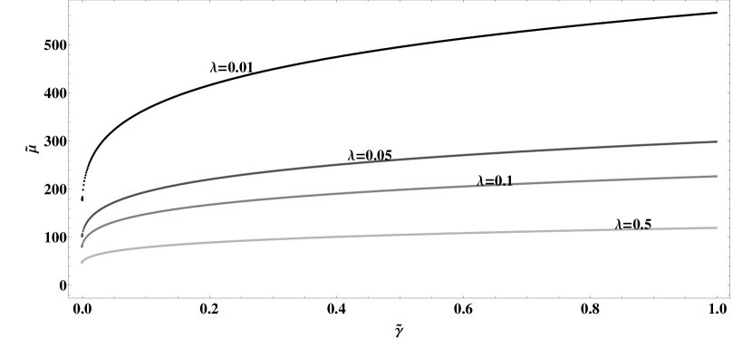
Figure 1: Chemical potential as a function of anharmonic term $\gamma$ for fixed number of atmos $N=1.0\times 10^{4}$. We fixed the temperature to be $k_{B}T=\hbar\omega_{r}$. Different lines represent different aspect ratios $\lambda$.

In this section we present thermodynamical properties as a function of temperature and trap potential parameters. For our calculations, we use a large number of atoms ($1.0\times 10^{4}$) to ensure the validity of our semi-classical treatment. First we solve Eq. 5 for $\tilde{\mu}$ for given $N$, $T$, and $\lambda$. As can be seen from FIG. 1, while the chemical potential increases with the anharmonic term, it decreases as the aspect ratio($\lambda$) increases. As more energy is needed to excite the fermions in low aspect ratio traps, the chemical potential in low aspect ratio traps is larger than that of higher aspect ratio traps. As we are using large number of atoms for our calculations, anharmonic term cannot be too negative. If the anharmonic term is too negative relative to the harmonic confinement, the trapped atoms cannot be confined as the potential is not bounded from below. The value of the anharmonicity at the point where it dominates over the harmonic confinement will be called critical anharmonicity hereafter. This critical anharmonicity depends on the number of atoms in the trap. For a set of representative parameters, this critical anharmonic value as a function of atom number is given in FIG. 2. Chemical potential for a range of negative anharmonic potential is given in FIG. 3.

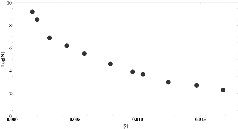
Figure 2: The critical negative anharmonic dependence on number of atoms in the trap for $k_{B}T=\hbar\omega_{r}$ and $\lambda$ =1. The atomic cloud is unstable below this critical value.

Figure 3: Chemical potential for negative anharmonic potentials. We fixed the temperature, number of atoms, and aspect ratio to be $k_{B}T=\hbar\omega_{r}$, $N=1.0\times 10^{4}$, and $\lambda=0.5$. For $\tilde{\gamma}<-0.001$, the system is unstable.

In FIG. 4, we plot the total energy as a function of anharmonic term. For given values of atomic number $N$, temperature $T$, and aspect ration $\lambda$, we first calculate the chemical potential from Eq. 9, and then we use this chemical potential to calculate the energy from Eq. 10. As can be seen in FIG. 4, for fixed number of atoms and fixed aspect ratio $\lambda$, dimensionless energy increases as we increase the anharmonic term $\gamma$. This is because of the trapping potential energy increases with increasing $\gamma$.

Figure 4: Total energy as function of anharmonic term $\gamma$ for fixed number of atmos $N=1.0\times 10^{4}$. We fixed the temperature to be $k_{B}T=\hbar\omega_{r}$ and the aspect ratio $\lambda$ = 0.5. For these selected parameters, absolute value of critical $|\gamma|$ is 0.001.

The low temperature behavior of the heat capacity calculated from Eq. (20) is shown in FIGS. 5-7. The temperature dependence of the heat capacity for different values of $\gamma$ and $\lambda$ is shown in FIG. 5 and FIG. 6. As we have considered up to the linear order in temperature, the specific heat is linear with temperature, however, the slope change significantly as we change the values of $\gamma$ or $\lambda$. The heat capacity of the polarized Fermi gas increases monotonically as the temperature increases. This behavior is completely different from a Bose gas cb where the heat capacity shows a maximum at supefluid-normal phase transition point. As can be seen from the figures, the heat capacity decreases with increasing anharmonic term $\gamma$. This decrease is due to the confinement effects which can be clearly seen from Eq. 20.

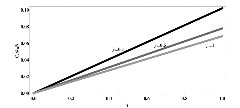
Figure 5: Specific heat as function of temperature for fixed number of atmos $N=1.0\times 10^{4}$. We fixed the aspect ratio to be $\lambda=0.5$.

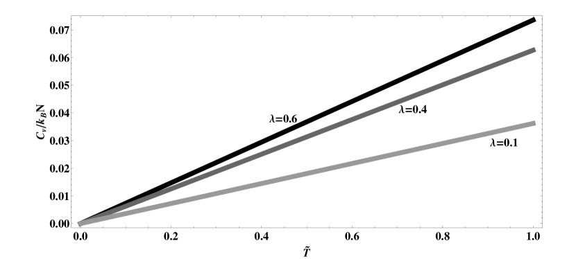
Figure 6: Specific heat as function of temperature for fixed number of atmos $N=1.0\times 10^{4}$ and $\tilde{\gamma}$ = 0.5.

Figure 7: Specific heat as function of $\gamma$ for negative $\gamma$’s. We fixed the number of atmos $N=1\times 10^{4}$. We fixed the $k_{B}T=\hbar\omega_{r}$.

IV IV. Conclusions

We have considered a spin-polarized Fermi gas trapped in an anharmonic potential. Applying a semiclassical treatment to the particle number and energy, and using a low-temperature series expansion method, we have derived analytical expressions for several thermodynamic quantities. We have discussed the trap parameter dependence on these quantities and the results were presented as a function of anharmonic trap parameter and temperature. The results of our paper can be tested in a lab by a similar experimental procedure carried out by Bretin et al. dali for Bose-Einstein condensates in a quartic trap.

In the present work, we considered fully polarized fermions. At low temperatures and low densities, s-wave short-range interactions are prohibited and higher wave scattering are strongly suppressed. The most natural extension of this work would be the inclusion of interaction. This can be done by adding another Zeeman state of atoms and consider the system as a two component fermions. A particular interesting regime is so called uintarity regime, where the scattering length between atoms is infinite. This regime is located near the Feshbach resonance fb . At this point, the interaction parameter disappears from the physical quantities. Therefore, all thermodynamic quantities are universal function of the dimensionless temperature $k_{B}T/\epsilon_{F}$, where $\epsilon_{F}$ is the Fermi energy ho . However, as there is no small parameter, it is difficult to reliably calculate thermodynamic quantities close the the unitarity regime. Therefore, one has to rely on good experimental data of energy, heat capacity, etc. duke . Then by comparing experimental data at unitarity regime with non-interacting calculation of thermodynamic quantities allows one to find the scaling factors. An accurate determination of these scaling factors of unitary Fermi gases is one of the challenging and fascinating theoretical problem at the moment mc .

References

- (1) M. H. Anderson, J. R. Ensher, M. R. Matthews, C. E. Wieman, E. A. Cornell, Science 269, 198-201, (1995); K.B. Davis, M.-O. Mewes, M.R. Andrews, N.J. van Druten, D.S. Durfee, D.M. Kurn, and W. Ketterle, Phys. Rev. Lett. 75, 3969, (1995); C. C. Bradley, C. A. Sackett, J. J. Tollett, and R. G. Hulet, Phy. Rev. Lett. 75, 1687 (1995); B. DeMarco, D. S. Jin, Science 285, 1703-1706 (1999); A. G. Truscott, K. E. Strecker, W. I. McAlexander, G. B. Partridge, R. G. Hulet, Science 291, 2570-2572 (2001); K. M. O’Hara, S. L. Hemmer, M. E. Gehm, S. R. Granade, J. E. Thomas, Science 298, 2179-2182, (2002); C. A. Regal, M. Greiner, and D. S. Jin, Phys. Rev. Lett. 92, 040403 (2004); M. W. Zwierlein, C. A. Stan, C. H. Schunck, S. M. F. Raupach, A. J. Kerman, and W. Ketterle, Phys. Rev. Lett. 92, 120403 (2004); C. Chin et al., Science 305, 1128-1130 (2004); T. Bourdel, L. Khaykovich, J. Cubizolles, J. Zhang, F. Chevy, M. Teichmann, L. Tarruell, S. J. J. M. F. Kokkelmans, and C. Salomon, Phys. Rev. Lett. 93, 050401 (2004); J. Kinast, S. L. Hemmer, M. E. Gehm, A. Turlapov, and J. E. Thomas, Phys. Rev. Lett. 92, 150402 (2004); J J. Kinast, S. L. Hemmer, M. E. Gehm, A. Turlapov, and J. E. Thomas, Phys. Rev. Lett. 92, 150402 (2004); M. Bartenstein, A. Altmeyer, S. Riedl, S. Jochim, C. Chin, J. H. Denschlag, R. Grimm, Phys. Rev. Lett. 92, 203201 (2004).
- (2) A. L. Fetter, Phys. Rev. A 64, 063608 (2001).
- (3) V. Bretin, S. Stock, Y. Seurin, and J. Dalibard, Phys. Rev. Lett. 92, 050403 (2004).
- (4) H. Zhai and T. -L. Ho, Phy. Rev. Lett. 97, 180414 (2006); M. Y. Veillette, D. E. Sheehy, L. Radzihovsky, and V. Gurarie, Phys. Rev. Lett. 97, 250401 (2006); G. Moller and N. R. Cooper, Phys. Rev. Lett. 99, 190409 (2007); N. R. Cooper, N. K. Wilkin, and J. M. Gunn, Phys. Rev. Lett. 87, 120405 (2001); B. paredes, P. Zoller, and J. I. Cirac, Sol. S. Com. 127, 155 (2003).
- (5) V. Bretin, S. Stock, Y. Seurin, J. Dalibard, Phys. Rev. Lett. 92, 050403 (2004)
- (6) G. M. Bruun and K. Burnett, Phys. Rev. A 58 (1998); E. J. Mueller, Phys. Rev. Lett. 93, 190404 (2004); X. X. Yi and J. C. Su, Physica Scripta, 60, 117 (1999); L. Salasnich, B. Pozzi, A. Parola, and L. Reatto, J. Phys. B: At. Mol. Opt. Phys. 33, 3943 (2000).
- (7) K. Howe, A. R. P. Lima, and A. Pelster, Eur. Phys. J. D 54 (2009).
- (8) T. N. De Silva. Phys. Rev. A 78, 023623 (2008).
- (9) E. Lundh, Phys. Rev. A 65, 043604 (2002); K. Kasamatsu, M. Tsubota, and M. Ueda, Phys. Rev. A 66, 053606 (2002); G. Kavoulakis and G. Baym, New J. Phys. 5, 51 (2003); E. Lundh, A. Collin, and K. A. Suominen, Phys. Rev. Lett. 92, 070401 (2004); T. K. Ghosh, Phys. Rev. A 69, 043606 (2004); T. K. Ghosh, Eur. Phys. J. D 31, 101 (2004); G. M. Kavoulakis, A. D. Jackson, and Gordon Baym, Phys. Rev. A 70, 043603 (2004); I. Danaila, Phys. Rev. A 72, 013605 (2005); A. Collin, Phys. Rev. A 73, 013611 (2006); S. Bargi, G. M. Kavoulakis, and S. M. Reimann, Phys. Rev. A 73, 033613 (2006); Michiel Snoek and H. T. Stoof, Phys. Rev. A 74, 033615 (2006); S. Gautam, D. Angom, Eur. Phys. J. D 46, 151 155 (2008).
- (10) R.K. Pathria, Statistical Mechanics, 2nd ed., Page 510 (Butterworth-Heinemann, 1996).
- (11) S. Kling and A. Pelster, Phys. Rev. A 76, 023609 (2007).
- (12) U. Fano, Phys. Rev. 124, 1866 (1961); H. Feshbach, Ann. Phys. 5, 357 (1958).
- (13) T. -L. Ho, Phys. Rev. Lett. 92, 090402 (2004).
- (14) J. Kinast, A. Turlapov, J. E. Thomas, Q. Chen2 J. Stajic, and K. Levin, Science, 307, 1296-1299 (2005).
- (15) J. Carlson et al., Phys. Rev. Lett. 91, 050401 (2003); S. Y. Chang et al., Phys. Rev. A 70, 043602 (2004); J. Carlson and S. Reddy, Phys. Rev. Lett. 95, 060401 (2005); G. E. Astrakharchik et al., Phys. Rev. Lett. 93, 200404 (2004); A. Bulgac, J. E. Drut, and P. Magierski, Phys. Rev. Lett. 96, 090404 (2006); A. Bulgac, J. E. Drut, and P. Magierski Phys. Rev. Lett. 99, 120401 (2007).