On Moduli Stabilisation and de Sitter Vacua in MSSM Heterotic Orbifolds

Abstract:

We study the problem of moduli stabilisation in explicit heterotic orbifold compactifications, whose spectra contain the MSSM plus some vector-like exotics that can be decoupled. Considering all the bulk moduli, we obtain the 4D low energy effective action for the compactification, which has contributions from various, computable, perturbative and non-perturbative effects. Hidden sector gaugino condensation and string worldsheet instantons result in a combination of racetrack, KKLT-like and cusp-form contributions to the superpotential, which lift all the bulk moduli directions. We point out the properties observed in our concrete models, which tend to be missed when only “generic” features of a model are assumed. We search for interesting vacua and find several de Sitter solutions, but so far, they all turn out to be unstable.

1 Introduction

In searching for the Standard Model (SM) of particle physics and its supersymmetric generalisations within String Theory, a myriad of constructions have been explored. Promising models have been built using heterotic orbifold compactifications, intersecting D-branes or D-branes at singularities and F-theory GUTs, to name a few. What all these models have in common, is that progress was made by focussing on the realisation of phenomenologically viable gauge groups and chiral matter spectra and, in particular, by neglecting gravity and the dynamics of the compactification.

Eventually, however, it will be necessary to embed the supersymmetric standard model (SSM) into globally consistent and stable string theory constructions. For example, supersymmetry breaking is usually associated with the dynamics of the moduli, and therefore in order to make predictions for the soft masses we require an understanding of how the moduli are stabilised. Ideas abound also in how to address the moduli stabilisation problem, and some progress has also been made towards dove-tailing these constructions with those of the SSM, particularly in Type IIB models [1]. So far though, the possibility of realising the SSM in a genuine metastable string compactification seems out of reach.

In this paper we continue towards this objective within the context of heterotic orbifold compactifications. Heterotic orbifolds are arguably amongst the simplest frameworks for such studies. They have had a long history as candidates for realistic string theory constructions, particularly in the eighties and nineties, and as such, much effort was also put towards understanding supersymmetry breaking and moduli stabilisation there. Recent years have seen a significant revival in this class of models, since it was realised that the idea of orbifold GUTs applied to heterotic orbifolds makes an effective tool to uncover the MSSM in the latter [2].

This progress is marked by the studies of a particularly fertile patch in the heterotic landscape, in which around 300 models were found containing the MSSM spectrum, together with only some vector-like exotics that can be decoupled [3]. They are built using a $\mathbbm{Z}_{6}$–II orbifold compactification, with a non-standard gauge embedding (leading to ${\mathcal{N}}=(0,2)$ worldsheet supersymmetry) and some number of discrete Wilson lines. We shall consider the problem of moduli stabilisation in some of these concrete promising models.

In their totality, these models contain, as well as the MSSM and the supergravity multiplets, a hidden gauge sector, a number of vector-like exotics, SM singlets (typically charged at least under Abelian factors of the hidden gauge sector), and the bulk moduli. Amongst the twisted fields there are also flat directions, and some of these may have a geometric interpretation as blow-up modes. The latter are known as twisted moduli, but, interestingly for the possibility that our universe is an orbifold, they are not always present [4]. As a first step, our focus will be on all the bulk moduli. Therefore, although we will begin by treating all degrees of freedom, at the end we shall assume that the vector-like exotics and SM singlets are decoupled at some scale close to the string scale, consistently with supersymmetry, e.g. due to dynamics such as those discussed in [3].

In order to study the bulk moduli dynamics, it is first necessary to construct the low energy effective field theory for the given orbifold compactification. Fortunately, there is a good knowledge of the effective Lagrangian for orbifold compactifications (for some nice reviews see [5, 6]). The relevant quantities can be computed using dimensional reduction and conformal field theory techniques [7, 8]. Another powerful tool [9, 10, 11] is modular invariance, which in the simplest models corresponds to an $SL(2,\mathbbm{Z})$ symmetry for each geometric modulus, and which is expected to hold even non-perturbatively. In what follows we shall compute the leading terms in the low energy effective field theory that describes concrete MSSM orbifold compactifications. Then, building on the work of the eighties and nineties, since all directions can be lifted, it seems natural to expect that (meta)stable vacua can exist.

Indeed, although the dilaton and geometric moduli are all flat directions at tree level, non-perturbative effects tend to lift them all. Since the dilaton describes the tree level gauge couplings, gaugino condensation in a hidden non-Abelian sector leads to a non-trivial potential for that field [12]. A racetrack potential [14, 15, 13] or KKLT-type potential [16, 17, 18] may then be sufficient to stabilise it. The gauge couplings also receive threshold corrections from massive string states that depend, via certain cusp-forms, on several of the Kähler moduli and all the complex structure moduli [8, 19], and thus a gaugino condensate may also stabilise those fields or even force compactification [20, 21, 15, 22]. Yukawa couplings between twisted fields arise thanks to worldsheet instantons [7], and are suppressed with the Kähler moduli that describe their separation. This lifts all the remaining Kähler moduli directions [23]. The most complete and general analysis to date on some of these effects can be found in the seminal work [15], which showed the success of racetrack dilaton stabilisation in the presence of hidden matter, together with the stabilisation of a universal Kähler modulus. Another interesting explicit analysis was performed in [22], where it was shown that a single gaugino condensate is sufficient to stabilise several geometrical moduli via a cusp-form mechanism, although the vacuum expectation value (vev) of the dilaton was set by hand.

The present work is a first attempt at treating all the bulk moduli together in explicit models that give rise to the MSSM. Our models have three Kähler moduli, one complex structure modulus plus the dilaton, giving a total of 10 real degrees of freedom. The various ingredients just described, give rise to a superpotential for all the fields, composed of a mixture of three types of terms, which have often been used in three popular stabilisation mechanisms: racetrack, KKLT and cusp-form stabilisation.

Several differences occur when considering concrete models compared to the inspiring toy models of the past, however. Some of these are: (i) the terms in the action are almost completely determined with very few free parameters (which come mainly from the little studied physics that decouples exotics), (ii) the modular symmetry groups are generically broken from $SL(2,\mathbbm{Z})$ to some congruence subgroup due to the presence of Wilson lines [24, 25], (iii) it is typically difficult to find more than one condensing gauge group, especially without decoupling hidden matter (since the latter tends to destroy asymptotic freedom), and subsequently, it is hard (but not impossible) to find dilatonic racetrack models, (iv) the moduli-dependent threshold corrections to the gauge couplings often do not appear with the required sign to force compactification, (v) it is not justified to take a universal Kähler modulus, and moreover the dynamics of all the bulk moduli are highly coupled together. All these features make the search for a metastable (de Sitter) vacuum more challenging than previously thought and our results underline this.

Due to the complexity of the system, our search for minima is largely numerical. We do find many de Sitter vacua, but all of them have unstable directions. We study their properties, including the presence of almost flat directions. Whether or not a metastable de Sitter vacuum might be waiting to be found is currently under investigation.

The organisation of the paper is as follows. In the next section, we review briefly the orbifold construction in heterotic strings. Expert orbifolders can skip this introduction, and go directly to Section 3, where we describe the low energy effective theory arising from generic heterotic orbifolds, which takes the form of an ${\mathcal{N}}=1$ supergravity. In particular, we recount the various perturbative and non-perturbative effects that can contribute to the dynamics of the moduli. Building on this discussion, Section 4 is devoted to the detailed study of the problem of moduli stabilisation in two concrete $\mathbbm{Z}_{6}$–II orbifold models, which contain the MSSM. We present explicit de Sitter vacua. Finally in Section 5 we discuss our results and the prospects to resolve the important open questions.

Throughout the paper we take $\kappa_{4}=1$ and use dimensionless quantities. Whenever units are necessary, we say so explicitly.

2 An Invitation to Heterotic Orbifolds

In this section we review briefly the compactification of the $\mathrm{E}_{8}$$\times$$\mathrm{E}_{8}$ heterotic string on non-freely acting, symmetric $\mathbbm{Z}_{N}$ toroidal orbifolds [6, 5], which are the setting for our investigation.

An orbifold is obtained by modding out a discrete set of isometries $P$ of a 6D torus $T^{6}$, characterised by a lattice $\Lambda$. $P$ is called the point group and we assume the torus $T^{6}$ to be factorisable, i.e. $T^{6}=T^{2}\times T^{2}\times T^{2}$. In general, the basis vectors $e_{\alpha}$ of the lattice $\Lambda$ can be chosen to be the simple roots of a Lie group, whose metric is $g_{\alpha\beta}=e_{\alpha}\cdot e_{\beta}$. The action of the point group generator $\vartheta$ on $\Lambda$ is given by

$$\vartheta\,:~{}e_{\alpha}\rightarrow e_{\beta}\ \Theta_{\beta\alpha}\,,$$ (1)

where $\Theta$ is the Coxeter element of the corresponding Lie algebra. In terms of the lattice metric, Eq. (1) becomes

$$\vartheta\,:~{}g_{\alpha\beta}\rightarrow\Theta^{T}g_{\alpha\beta}\Theta\,.$$ (2)

An admissible lattice should be invariant under $P$. This restricts the choice of $\Lambda$, but leaves some free parameters, which correspond to the geometric moduli of the compactification.

In $\mathbbm{Z}_{N}$ orbifolds, the generator $\vartheta$ can be made diagonal, such that

$$\vartheta=\mathrm{diag}(e^{2\pi\mathrm{i}v_{1}},\,e^{2\pi\mathrm{i}v_{2}},\,e^{2\pi\mathrm{i}v_{3}})$$

where $v=(0,\,v_{1},\,v_{2},\,v_{3})$ is the twist vector that parametrises the action of the orbifold on the compact space . Since $\vartheta$ is of order $N$, it follows that $N\,v_{i}=0\mod 1$. Additionally, $v$ is subject to the constraint $\sum_{i}v_{i}=0$ that guarantees the holonomy to be a (discrete) subgroup of $\mathrm{SU}(3)$ (but larger than $\mathrm{SU}(2)$) and consequently, $\mathcal{N}=1$ in 4D.

In the bosonic formulation, points of the torus are given by six real or, equivalently, three complex coordinates $Z_{i}$, $i=1,2,3$. Under $\vartheta$, the torus coordinates transform as

$$Z_{i}\stackrel{{\scriptstyle\vartheta}}{{\longrightarrow}}\vartheta_{i}Z_{i}\,.$$ (3)

In order to include the fact that $Z$ is a point on $T^{6}$, i.e. $Z\equiv Z+\lambda$ with $\lambda\in\Lambda$, it is customary to define the space group $S$ as the semidirect product $S=P\ltimes\Lambda$. An arbitrary space group element $g=(\vartheta^{k},\,n_{\alpha}e_{\alpha})$ acts then on the coordinates of the compact space as

$$Z\stackrel{{\scriptstyle g}}{{\longrightarrow}}\vartheta^{k}Z+n_{\alpha}e_{\alpha},\quad\qquad n_{\alpha}\in\mathbbm{Z}\,.$$ (4)

It is easy to see that the action of a non-trivial space group element leaves invariant the points $f$ satisfying

$$(\mathbbm{1}-\vartheta^{k})\,f=n_{\alpha}e_{\alpha},\quad\qquad n_{\alpha}\in\mathbbm{Z}\,.$$ (5)

Such points are called fixed points. Sometimes, instead of $f$, one uses the associated space group element $g$ to refer to the fixed points. Since all elements from the conjugacy class of $g$, defined as $\{h\,g\,h^{-1}\,|\,h\in S\}$, have an equivalent action on the compact space, then the corresponding fixed points are equivalent in the orbifold.

For each point group element $\vartheta^{k}$, one obtains a different number of inequivalent fixed points. Therefore, usually one refers collectively to the set of fixed points for a given $k$ as the $\vartheta^{k}$ twisted sector. For $k=0$, the twist action is trivial and therefore there are no fixed points. This sector is called the untwisted sector. The action of the point group on the $\vartheta^{k}$ twisted sector is conveniently encoded in the local twist vector $\boldsymbol{k}=k\,v$. In orbifolds with non-prime $N$, there are some sectors in which the twist acts trivially on one of the three two-torii. In these cases, we get fixed torii instead of fixed points. The holonomy in these sectors is a subgroup of $\mathrm{SU}(2)$, which leaves $\mathcal{N}=2$ supersymmetry unbroken.

Modular invariance requires the action of the space group to be accompanied by a corresponding action on the 16 gauge degrees of freedom $X_{I}$ of the heterotic string. The action of $\vartheta$ can be described by a shift 

$$X\stackrel{{\scriptstyle\vartheta}}{{\longrightarrow}}X+\pi V\,,$$ (6)

where $V$ is the shift vector. The lattice translations $e_{\alpha}$ are translated to the gauge degrees of freedom as discrete Wilson lines ${\cal A}_{\alpha}$. Thus, an arbitrary space group element $g=(\vartheta^{k},\,n_{\alpha}e_{\alpha})$ affects the gauge degrees of freedom as

$$X\stackrel{{\scriptstyle g}}{{\longrightarrow}}X+\pi(k\,V+n_{\alpha}{\cal A}_{\alpha})\,.$$ (7)

Not every shift and Wilson lines are compatible with the space group. First, from $\vartheta^{N}=\mathbbm{1}$ it follows that $N\,V$ must be a vector in the weight lattice of $\mathrm{E}_{8}$$\times$$\mathrm{E}_{8}$, i.e. the shift has to be of order $N$ too. Also the Wilson lines are constrained. Since the space group elements $g=(\mathbbm{1},\,n_{\alpha}e_{\alpha})$ and $\vartheta^{\ell}\,g\,\vartheta^{-\ell}=(\mathbbm{1},\,\vartheta^{\ell}n_{\alpha}e_{\alpha})\equiv(\mathbbm{1},\,m_{\beta}e_{\beta})$ are in the same conjugacy class, the Wilson lines $n_{\alpha}{\cal A}_{\alpha}$ and $m_{\beta}{\cal A}_{\beta}$ must coincide. Direct consequences of this are that not all the Wilson lines are non-trivial nor independent, they can take only quantised values, and their order $N_{\alpha}$ is restricted by the geometry of the compact space.

Demanding modular invariance of the one-loop vacuum-to-vacuum amplitudes imposes additional constraints on the orbifold parameters which, for $\mathbbm{Z}_{N}$ orbifolds without Wilson lines, read [26]

$$N(V^{2}-v^{2})=0\mod 2\,.$$ (8)

In the presence of non-trivial Wilson lines, Eq. (8) has to be amended by [27] (no summation implied)

$$N_{\alpha}\,{\cal A}_{\alpha}\cdot V = 0\mod 2\,,$$ (9a)

$$N_{\alpha}\,{\cal A}_{\alpha}^{2} = 0\mod 2\,,$$ (9b)

$$\gcd(N_{\alpha},N_{\beta})\,{\cal A}_{\alpha}\cdot{\cal A}_{\beta} = 0\mod 2\qquad(\alpha\neq\beta)\,,$$ (9c)

where $\gcd$ stands for the greatest common denominator. These conditions guarantee anomaly freedom of the low energy effective theory.

The simplest gauge embedding of the orbifold action corresponds to identifying the shift vector $V$ with the twist vector $v$ and setting ${\cal A}_{\alpha}=0$ or, in the context of supergravity, to embed the spin connection into the gauge connection. This is the trivial solution to the modular invariance condition (8) and it is called standard embedding (SE). On the string theory side, the standard embedding preserves $(2,2)$ worldsheet supersymmetry. From the phenomenological point of view, the SE is not very attractive, since it is not possible to get realistic spectra . Therefore, we work with non-trivial solutions to  (8), or non-standard embedding (NSE) models. On the string theory side, these correspond to $(0,2)$ supersymmetric theories on the worldsheet. Moreover, also from phenomenological requirements, we are interested in models with non-trivial discrete Wilson lines. Indeed, all orbifold models with promising phenomenological properties correspond to this category [3]. We describe below the massless spectrum of this type of models.

2.1 Massless orbifold spectrum

The massless spectrum of an orbifold is comprised of two kinds of closed strings. The untwisted states stem from the original spectrum of closed strings of the heterotic string. In the supergravity limit, they correspond to the components of the 10D supergravity multiplet and the $\mathrm{E}_{8}$$\times$$\mathrm{E}_{8}$ vector multiplets that are left invariant by the orbifold action. The twisted states arise from closed strings attached to the fixed points. These strings exist only due to the orbifold, i.e. they cannot be identified as part of the supergravity limit of the heterotic string. It is natural to associate each state with a space group element commonly called constructing element. E.g. states in the untwisted sector are “constructed” by the element $(\mathbbm{1},\,0)$ whereas those lying at the fixed point of the origin in the $k=2$ twisted sector are associated with $(\vartheta^{2},\,0)$.

The general form of an orbifold state associated with $g=(\vartheta^{k},\,n_{\alpha}e_{\alpha})$ can be written as

$$|\psi\rangle=|q_{\rm sh}\rangle_{R}\otimes\beta\,|p_{sh}\rangle_{L}\otimes|f\rangle\,.$$ (10)

In this formalism, $q_{\rm sh}=q+\boldsymbol{k}$ encodes the quantum numbers of the (right-moving) string in the physical degrees of freedom of the compact and Minkowski space, where $q$ is an $\mathrm{SO}(8)$ weight (e.g. for $k=0$ $q$ is a weight of either $\boldsymbol{8}_{v}$ or $\boldsymbol{8}_{s}$) and $\boldsymbol{k}=k\,v$ is the local twist vector defined above. $\beta$ denotes a product of (left-moving) oscillator excitations $\widetilde{\beta}^{I}_{-1}$ in the 16 gauge dimensions, $\widetilde{\beta}^{\mu}_{-1}$ in the Minkowski space, $\widetilde{\beta}^{i}_{-\eta_{i}}$ and $\widetilde{\beta}^{\bar{\imath}}_{-1+\eta_{i}}$ in the holomorphic $i$ and antiholomorphic $\bar{\imath}$ directions of the compact space, respectively. Here $\eta_{i}=\boldsymbol{k}_{i}\mod 1$, such that $0<\eta_{i}\leq 1$. Further, $p_{\rm sh}=p+k\,V+n_{\alpha}\,{\cal A}_{\alpha}$ (with $p$ a weight of $\mathrm{E}_{8}$$\times$$\mathrm{E}_{8}$) is a 16D vector that carries the information on the gauge quantum numbers. Finally, the component $|f\rangle$ contains the geometric information regarding the localisation in the compact space of the orbifold state.

The quantum numbers of a massless state must fulfill

$$\begin{array}[]{rl}\frac{1}{4}m_{L}^{2}=&\frac{1}{2}p^{2}_{\rm sh}+\widetilde{N}-1+\delta c\stackrel{{\scriptstyle!}}{{=}}0\,,\\[5.69054pt] \frac{1}{4}m_{R}^{2}=&\frac{1}{2}q^{2}_{\rm sh}-\frac{1}{2}+\delta c\stackrel{{\scriptstyle!}}{{=}}0\,,\end{array}$$ (11)

where $\delta c=\frac{1}{2}\sum_{i}\eta_{i}(1-\eta_{i})$ corresponds to a change in the zero point energy due to (twisted) oscillators. The oscillator number $\widetilde{N}$ is given by

$$\widetilde{N}=\sum_{i=1}^{3}\eta_{i}\widetilde{N}^{i}_{g}+\bar{\eta}_{i}\widetilde{N}^{*i}_{g}$$ (12)

with $\bar{\eta}_{i}=-\boldsymbol{k}_{i}\mod 1$, such that $0<\bar{\eta}_{i}\leq 1$. Here, $\widetilde{N}^{i}_{g}$ and $\widetilde{N}^{*i}_{g}$ count the number of excitations related to the constructing element $g$ in the $i$ and $\bar{\imath}$ directions.

Massless states $|\psi\rangle$ with constructing element $g=(\vartheta^{k},\,n_{\alpha}e_{\alpha})$ acquire in general a non-trivial phase under the action of an arbitrary space group element $h=(\vartheta^{l},\,m_{\alpha}e_{\alpha})$,

$$|\psi\rangle\stackrel{{\scriptstyle h}}{{\longrightarrow}}e^{2\pi\mathrm{i}\,[p_{\text{sh}}\cdot(lV+m_{\alpha}{\cal A}_{\alpha})-{\mathcal{R}}\cdot lv-\frac{1}{2}\,\left((kV+n_{\alpha}{\cal A}_{\alpha})\cdot(lV+m_{\alpha}{\cal A}_{\alpha})-\boldsymbol{k}\cdot lv\right)]}\,|\psi\rangle\,,$$ (13)

where we have defined the vector of ${\mathcal{R}}$-charges

$${\mathcal{R}}=q_{\rm sh}-\widetilde{N}_{g}+\widetilde{N}^{*}_{g}\,.$$ (14)

The orbifold projection consists of letting space group elements $h$ such that $[g,h]=0$ act on the states $|\psi\rangle$. Only invariant states under this action are retained in the orbifold spectrum.

2.1.1 Untwisted sector

In the untwisted sector, $\boldsymbol{k}=0$ implies that the masslessness condition (11) reduces to

$$\frac{1}{2}p^{2}+\widetilde{N}-1=0=\frac{1}{2}q^{2}-\frac{1}{2}\,.$$ (15)

Therefore, the solutions to this equation are given by $q^{2}=1$ and $p^{2}=2,\,\widetilde{N}=0$ or $p^{2}=0,\,\widetilde{N}=1$. The resulting massless states can be gathered together in the following categories:

Gravity multiplet and dilaton.

The states of the form $|q\rangle_{R}\otimes\widetilde{\beta}_{-1}^{\mu}|0\rangle_{L}$ ($\mu$ runs in the Minkowski coordinates) such that $q\cdot v=0\mod 1$ correspond to a) the degrees of freedom of the graviton $g^{\mu\nu}$, b) the dilaton $\phi$, and c) one surviving component of the 10D $B$ 2-form, whose dual is the so-called model independent axion, $a$. Since the orbifold preserves $\mathcal{N}=1$ supersymmetry, also the superpartners are included in this notation. We can build an $\mathcal{N}=1$ chiral supermultiplet from the dilaton and axion, whose bosonic component is given by

$$S=\sqrt{\det g}\,e^{-2\phi}+ia$$ (16)

with $g$ the internal metric.

Geometric moduli.

The geometric moduli in the effective theory are the pure internal components of the 10D supergravity multiplet that survive the orbifold projection. In our notation, they are expressed as $|q\rangle_{R}\otimes\widetilde{\beta}_{-1}^{j}|0\rangle_{L}$ and $|q\rangle_{R}\otimes\widetilde{\beta}_{-1}^{\bar{\jmath}}|0\rangle_{L}$ with $(q-\widetilde{N}+\widetilde{N}^{*})\cdot v=0\mod 1$. Traditionally, the states $|q\rangle$ have been denoted as $|i\rangle$ or $|\bar{\imath}\rangle$ depending on the position and sign of the vectorial $\mathrm{SO}(8)$ weight $q$. For instance, $|1\rangle$ denotes $q=(0,1,0,0)$ and $|\bar{2}\rangle$ denotes $q=(0,0,-1,0)$. In this notation, states with $|q\rangle=|i\rangle$ and antiholomorphic oscillator index $\bar{\jmath}$ are the $h^{1,1}$ Kähler moduli. Since we will be working in the case with one Kähler modulus per 2-torus, then $i$ and $j$ coincide and the moduli are denoted as $T_{i}$. States with $|q\rangle=|i\rangle$ and holomorphic oscillator index $j$ are the $h^{2,1}$ complex structure moduli $U$.

A more useful notation to illustrate the geometric origin of these moduli is achieved through the torus metric. This can be rewritten as $g_{\alpha\beta}=e_{\alpha}\cdot e_{\beta}=R_{\alpha}R_{\beta}\cos\varphi_{\alpha\beta}$, with $R_{\alpha}$ being the “radius” of the cycle $e_{\alpha}$, and $\varphi_{\alpha\beta}$ the angle between $e_{\alpha}$ and $e_{\beta}$. According to Eq. (2), imposing $P$ invariance amounts to requiring

$$\Theta^{T}g_{\alpha\beta}\Theta=g_{\alpha\beta}\,.$$ (17)

This requirement fixes some of the parameters $R_{\alpha}$ and $\varphi_{\alpha\beta}$. The remaining free parameters are combined to build the $h^{2,1}$ Kähler moduli and $h^{1,1}$ complex structure moduli. To this purpose, let us define the metric of the $i^{th}$ $T^{2}_{(i)}$ plane as

$$g^{(i)}\equiv\left(\begin{array}[]{cc}g_{2i-1,\,2i-1}&g_{2i-1,\,2i}\\ g_{2i-1,\,2i}&g_{2i,\,2i}\\ \end{array}\right)\,.$$ (18)

In terms of this metric, the complex structure and Kähler moduli of the $i^{th}$ plane are given, respectively, by

$$U_{i}=\frac{\sqrt{\det g^{(i)}}}{g^{(i)}_{11}}+\mathrm{i}\,\frac{g^{(i)}_{12}}{g^{(i)}_{11}}\,,\qquad\qquad T_{i}=\frac{1}{2}\left(\sqrt{\det g^{(i)}}+\mathrm{i}B_{2i-1,2i}\right)\,.$$ (19)

Since $U_{i}$ contain only ratios of terms in the metric, they describe deformations in the shape of the 2-torii. Information about the overall size of the torii is carried by $T_{i}$.

4D gauge group.

The states of the form $|q\rangle_{R}\otimes|p\rangle$ with $q\cdot v=0\mod 1$ and $p\cdot V=0=p\cdot{\cal A}_{\alpha}$ together with the 16 Cartan generators of $\mathrm{E}_{8}$$\times$$\mathrm{E}_{8}$ $|q\rangle_{R}\otimes\widetilde{\beta}_{-1}^{I}|0\rangle_{L}$, $I=1,\ldots,16$, correspond to the gauge bosons of the unbroken 4D gauge group $G_{4D}$. Notice that since $\beta_{-1}^{I}|0\rangle_{L}$ does not transform under the orbifold action, the rank of the gauge group is always preserved . However, out of the 480 original charged gauge bosons ($p\neq 0$) only a subset of them survives the orbifold projection. Therefore, the gauge group is in general a subgroup of $\mathrm{E}_{8}$$\times$$\mathrm{E}_{8}$. For instance, SE induces the breaking $\mathrm{E}_{8}\rightarrow\mathrm{E}_{6}\times G_{2d}$, with $G_{2d}=\mathrm{SU}(3),\,\mathrm{SU}(2)\times\mathrm{U}(1)$ or $\mathrm{U}(1)^{2}$ depending on the $\mathbbm{Z}_{N}$ orbifold. In non-standard embedding with Wilson lines, the breaking takes a more complex form.

Chiral multiplets.

Untwisted charged matter arises from the states $|q\rangle_{R}\otimes|p\rangle$ where the orbifold projection is given by $p\cdot(lV+m_{\alpha}{\cal A}_{\alpha})-q\cdot lv=0\mod 1$ with arbitrary integers $l$ and $m_{\alpha}$. Their gauge transformation properties with respect to $G_{4D}$ are encoded in $p$.

2.1.2 Twisted sector

Zero modes of the $\vartheta^{k}$ twisted sectors ($k\neq 0$) are associated to the constructing elements $g=(\vartheta^{k},\,n_{\alpha}e_{\alpha})$ and, therefore, attached to the corresponding fixed points. These are matter states that take the form (10) and are constrained by the general masslessness condition (11). As before, their gauge transformation properties are encoded in the gauge momenta $p_{\rm sh}$. Note that, since at the fixed points the gauge symmetry can be larger than the one in 4D, from a local perspective, at the fixed points, the orbifold-invariant states transform as complete multiplets of the local gauge symmetry. This observation has been useful to develop the concept of local GUTs [2, 29, 30].

In the appendices we give the complete 4D massless spectrum for specific heterotic orbifold compactifications. For all models of interest, the spectrum is composed of the supergravity multiplet and the MSSM spectrum, together with some “hidden” gauge groups, hidden matter, a number of vector-like exotic matter multiplets and the bulk moduli.

2.2 String selection rules

Couplings among matter fields are constrained by the symmetries of the orbifold. All invariant interactions with non-vanishing strength can be identified by using the so-called selection rules [7, 31], which arise from those symmetries. In this discussion , we consider the coupling $c=\prod_{\alpha}A_{\alpha}$, where the matter fields $A_{\alpha}$ are characterised by the gauge momenta $p_{{\rm sh},\alpha}$, ${\mathcal{R}}$-charges ${\mathcal{R}}_{\alpha}$ and constructing element $g_{\alpha}$.

Gauge invariance.

Since the gauge quantum numbers of all matter states are encoded in the gauge momenta $p_{\rm sh}$, $c$ is gauge invariant as long as it fulfills

$$\sum_{\alpha}p_{{\rm sh},\alpha}=0\,.$$ (20)

${\mathcal{R}}$-charge conservation.

This selection rule of stringy origin arises from the discrete symmetries of the 6D compactification lattice $\Lambda$ that are left unbroken under the orbifold action. In factorisable orbifolds, $c$ preserves these symmetries if it satisfies

$$\sum_{\alpha}{\mathcal{R}}_{\alpha}^{i}=-1\mod N_{i}\,,\qquad\text{ for all }i\,,$$ (21)

where $N_{i}$ are the orders of the $T^{2}$ orbifold twists, i.e. $N_{i}$ are the smallest positive integers such that $N_{i}v_{i}=0\mod 1$ (no summation over $i$).

Space group selection rule.

String interactions are only possible if the closed strings involved can join and form other closed strings. The constructing element $g_{\alpha}$ not only characterises the fixed point $f_{\alpha}$ of the matter state $A_{\alpha}$ but also describes the boundary conditions of the associated strings. Based on this,

$$\prod_{\alpha}[g_{\alpha}]=(\mathbbm{1},\,0)\,,$$ (22)

where $[g_{\alpha}]$ denotes some element of the conjugacy class of $g_{\alpha}$. The rotational part of this equation reads $\prod_{k_{\alpha}}\vartheta^{k_{\alpha}}=\mathbbm{1}$ or analogously $\sum_{\alpha}k_{\alpha}=0\mod N$, which is called point group selection rule.

For trilinear couplings, it is convenient to express the space group selection rule in terms of the fixed points $f_{\alpha}$

$$(\mathbbm{1}-\Theta^{k_{\alpha}})(\Theta^{p}f_{\alpha}-\tau_{\alpha})+\Theta^{k_{\alpha}}(\mathbbm{1}-\Theta^{k_{\beta}})(\Theta^{q}f_{\beta}-\tau_{\beta})=(\mathbbm{1}-\Theta^{k_{\alpha}+k_{\beta}})\Theta^{r}f_{\gamma}\,,$$ (23)

where $\tau_{\alpha,\beta}$ are arbitrary lattice vectors and the integers $p,q,r$ lie between $0$ and $N/2$.

In the appendices, we give the Yukawa couplings allowed by the above selection rules for specific models.

3 Low Energy Effective Supergravity Theory

To study the dynamics of the moduli fields, we construct the low energy effective field theory, which describes the physics at energies well below the compactification scale. This is described by a 4D ${\mathcal{N}}=1$ supergravity theory and thus we must identify the corresponding Kähler potential, $K$, gauge kinetic functions, $f_{a}$, and superpotential, $W$.

For the purely untwisted fields of the orbifold compactification, the action can be identified simply by directly truncating the low energy 10D supergravity action describing the heterotic string. Things are a bit more complicated for twisted sectors, which emerge due to the compactification. The approach, pioneered in [7, 8], is to construct an effective field theory that yields the same scattering amplitudes as the full string theory does in the low energy limit. Since orbifolds represent exactly solvable superconformal field theories, all quantities can, in principle, be computed.

The low energy effective action receives corrections from two perturbative expansions: the string loop corrections, in $e^{2\phi}$, and the supergravity approximation, in $\alpha^{\prime}$. These corrections depend on the dilaton and volume moduli respectively. However, 4D ${\mathcal{N}}=1$ supersymmetry gives rise to powerful “non-renormalisation theorems”. The tree-level superpotential cannot receive corrections from (string loop or $\alpha^{\prime}$) perturbative effects, and is corrected only by non-perturbative effects [32]. Similarly, the gauge kinetic function receives string loop corrections only at one-loop, and no higher [33].

Finally, the low energy effective theory enjoys a further constraint from the discrete target-space modular invariance, which is inherited from the underlying conformal field theory. This provides a valuable check on all computations.

In this section, we first describe in detail the modular symmetry, and then present the terms of the low energy effective action for the light fields in a generic orbifold compactification. We consider the untwisted moduli, $S,T_{i},U_{m}$, gauge sector and matter fields, $A_{\alpha}$. When relevant, we distinguish between charged matter fields (charged under the SM or hidden non-abelian groups), $Q_{I}\subset A_{\alpha}$, and SM and non-abelian singlets (charged only under hidden $\mathrm{U}(1)$s), $\Phi_{\Gamma}\subset A_{\alpha}$.

3.1 Target space modular symmetry

The spectrum of states in an orbifold string compactification is invariant under certain discrete transformations on the moduli, together with the winding numbers and momenta. In the simplest orbifold compactifications, without Wilson lines, the corresponding target space duality group is $SL(2,\mathbb{Z})_{T}^{h_{(1,1)}}\times[SL(2,\mathbb{Z})]_{U}^{h_{(2,1)}}$. Under this symmetry, the moduli, $\phi_{j}=(T_{i},U_{m})$, and matter fields, $A_{\alpha}$, transform as follows  [34, 11]

$$\phi_{j}\rightarrow\frac{a_{j}\phi_{j}-\mathrm{i}b_{j}}{\mathrm{i}c_{j}\phi_{j}+d_{j}}\qquad a_{j},b_{j},c_{j},d_{j}\in\mathbbm{Z},\qquad a_{j}d_{j}-b_{j}c_{j}=1$$ (24)

$$A_{\alpha}\rightarrow M_{\alpha\beta}A_{\beta}\prod_{j}^{h^{1,2},h^{1,1}}(\mathrm{i}c_{j}\phi_{j}+d_{j})^{n_{\alpha}^{j}}\,.$$ (25)

The modular weights $n^{j}_{\alpha}=(n_{\alpha}^{i},\ell^{m}_{\alpha})$ are given by  [11]

$$n^{i}=\left\{\begin{array}[]{lcl}q_{{\rm sh},i}&\phantom{....}&\text{for }q_{{\rm sh},i}=0,-1\,,\\ -1-q_{{\rm sh},i}+\widetilde{N}_{g}^{i}-\widetilde{N}_{g}^{*i}&&\text{for }q_{{\rm sh},i}\neq 0,-1\,,\end{array}\right.$$ (26a)

and

$$\ell^{m}=\left\{\begin{array}[]{lcl}q_{{\rm sh},m}&\phantom{....}&\text{for }q_{{\rm sh},m}=0,-1\,,\\ -1-q_{{\rm sh},m}-\widetilde{N}_{g}^{m}+\widetilde{N}_{g}^{*m}&&\text{for }q_{{\rm sh},m}\neq 0,-1\,,\end{array}\right.$$ (26b)

where the internal momenta $q_{{\rm sh}}$ and oscillator numbers $\widetilde{N}_{g},\widetilde{N}_{g}^{*}$ have been defined in Section 2.1. The matrices $M_{\alpha\beta}$ are field-independent, and describe how the twisted fields with the same weights and charges transform amongst each other. Although in the supergravity basis this transformation is not unitary, it is so for the canonically normalised fields.

Together with the sigma-model symmetries, the target space modular symmetry can be anomalous. Part of this anomaly can be cancelled by a Green-Schwarz mechanism, which implies that the dilaton $S$ transforms at 1-loop, as [35]

$$S\rightarrow S-\frac{1}{8\pi^{2}}\sum_{j}^{h^{1,2},h^{1,1}}\delta_{GS}^{j}\log(\mathrm{i}c_{j}\phi_{j}+d_{j})\,,$$ (27)

where $\delta_{GS}^{j}$ are the gauge group independent Green-Schwarz coefficients describing 1-loop mixing between the dilaton and the geometric moduli. The remainder of the anomaly is cancelled by threshold corrections due to massive string states, which we discuss below.

The Kähler potential, $K$, transforms at both tree and 1-loop level as

$$K\rightarrow K+\sum_{j}^{h^{1,2},h^{1,1}}\log|\mathrm{i}c_{j}\phi_{j}+d_{j}|^{2}\,,$$ (28)

and, in order to obtain invariant matter couplings, the superpotential has to transform (up to a field-independent phase) as [23]

$$W\rightarrow\frac{W}{\prod_{j}^{h^{1,2},h^{1,1}}(\mathrm{i}c_{j}\phi_{j}+d_{j})}\,.$$ (29)

Modular invariance means that several terms in the action can be written in terms of modular forms, which transform covariantly with some weight ${\rm k}$. The most common of these is the well-known Dedekind eta function

$$\eta(\phi)=e^{-\pi\phi/12}\prod_{n=1}^{\infty}(1-e^{-2n\pi\phi})\,,$$ (30)

which is a cusp-form of weight ${\rm k}=1/2$. This means that it vanishes at real infinity  and its modular transformation reads (up to a field-independent phase factor)

$$\eta(\phi)\rightarrow(\mathrm{i}c\phi+d)^{1/2}\,\eta(\phi)\,.$$ (31)

The presence of discrete Wilson line backgrounds breaks the modular symmetries down to the subgroup that leaves the Wilson line invariant [24, 25]. Typically, the surviving modular symmetries are congruence subgroups of $SL(2,\mathbb{Z})$, which further restrict the integer parameters, $a,\,b,\,c,\,d$, of the transformations. They can be computed by solving the constraints found in [25]. For instance, the groups that we encounter below are

$$\Gamma_{0}(N):c=0\,\,{\rm{mod}}\,\,N$$ (32)

$$\Gamma^{0}(N):b=0\,\,{\rm{mod}}\,\,N\,\,$$ (33)

$$\Gamma_{1}(N):a,d=1\,\,{\rm{mod}}\,\,N\quad{\rm{and}}\,\,c=0\,\,{\rm{mod}}\,\,N\,\,$$ (34)

$$\Gamma^{1}(N):a,d=1\,\,{\rm{mod}}\,\,N\quad{\rm{and}}\,\,b=0\,\,{\rm{mod}}\,\,N$$ (35)

with of course also $a,b,c,d\in\mathbbm{Z}$ and $ad-bc=1$. It is easy to show  that, for instance, $\eta(N\phi)$ transforms covariantly under $\Gamma_{0}(N)$ but not under the full modular group $SL(2,\mathbb{Z})$. For $\Gamma^{0}(N)$, the corresponding function is $\eta(\phi/N)$.

We close this subsection by noting that modular invariance represents a powerful means to check the low energy effective theory that one computes. Moreover, identifying modular functions with the required weights and zero/singularity structure provides a way to infer the moduli-dependence of various terms in the action, when direct computations are lacking.

In the remainder of this section, we introduce the different contributions to the low energy $\mathcal{N}=1$ 4D effective theory below the compactification scale. When reviewing previous computations, we present only the final results and refer the reader to the original literature for further details.

3.2 Moduli and matter kinetic terms

The kinetic terms for the moduli and matter fields are encoded in the Kähler potential. For the twisted fields they have been computed to lowest order in the matter fields $A_{\alpha}$, with

$$|A_{\alpha}|^{2}\prod_{j}^{h^{1,1},h^{2,1}}(\phi_{j}+\bar{\phi}_{j})^{n_{\alpha}^{j}}\ll 1\,.$$ (36)

Then, including one-loop effects, we have [15, 23, 22, 11, 42]

$$\hskip-2.84544ptK = -\log\left[S+\bar{S}-\frac{1}{8\pi^{2}}\sum_{j}^{h^{1,1},h^{2,1}}\delta_{GS}^{j}\log(\phi_{j}+\bar{\phi}_{j})\right]$$ (37)

$$\hskip 85.35826pt-\sum_{j}^{h^{1,1},h^{2,1}}\log(\phi_{j}+\bar{\phi}_{j})+\,|A_{\alpha}|^{2}\prod_{j}^{h^{1,1},h^{2,1}}(\phi_{j}+\bar{\phi}_{j})^{n_{\alpha}^{j}}\,.$$

Here $n_{\alpha}^{j}$ are the modular weights as defined before. It is easy to show that (37) transforms in the required way (28) under the modular symmetry. The Kähler potential receives further perturbative corrections as well as non-perturbative ones. These, however, should be small compared with the leading contribution above.

3.3 Matter interactions

At tree-level, there may be couplings between bulk fields, bulk fields and twisted fields, or twisted fields located at the same fixed points. All these interactions can be understood within field theory, and are of order one. At the same time, recalling the stringy nature of the twisted fields, even though their center of masses are localised, they can stretch away from the corresponding fixed points. This leads to non-perturbative corrections to the interactions between twisted fields, which can be interpreted as world-sheet instantons and which are exponentially suppressed in the Kähler moduli that measure the area of the wrapped instantons.

We now discuss in detail the trilinear Yukawa couplings, and their contributions to the superpotential. Our focus here is on twisted fields only, which have a non-trivial dependence of the Kähler moduli. Then we briefly comment on the aspects of higher order couplings that are relevant for our purposes.

3.3.1 Yukawa couplings

The computation of trilinear Yukawa couplings was started in [7, 36] and completed in [37]. They were also explicitly computed for several orbifolds in [38].

Selection rules for permitted couplings were discussed in Section 2.2. A generic coupling allowed between three twisted fields from the sectors $(\vartheta^{k},\,\vartheta^{l},\,\vartheta^{-(k+l)})$, located respectively at fixed points $(f_{\alpha},\,f_{\beta},\,f_{\gamma})$, is given by ,

$$\hskip-56.9055ptY^{kl}_{\alpha\beta\gamma}=F_{\alpha\beta\gamma}g_{s}\,\sqrt{V_{\Lambda}}\sum_{u}\prod_{i\notin{\mathcal{J}}}\sqrt{2\pi}\sqrt{\Gamma_{\boldsymbol{k}_{i},\,\boldsymbol{l}_{i}}}\exp{\left(-\pi\,|\cot{\boldsymbol{k}_{i}\pi}+\cot{\boldsymbol{l}_{i}\pi}|^{-1}|u_{i}|^{2}\right)}\,,$$ (38)

where the local twists are $\boldsymbol{k}=k\,v$ and $\boldsymbol{l}=l\,v$, and $\mathcal{J}$ is the set of indices $j$ labelling invariant planes, with $\boldsymbol{k}_{j},\,\boldsymbol{l}_{j}$ or $\boldsymbol{k}_{j}+\boldsymbol{l}_{j}=0$ (mod 1). The summation is over the components of $u$ orthogonal to the planes $j\in{\mathcal{J}}$ and is due to contributions from fixed points equivalent to $f_{\alpha,\beta,\gamma}$ thanks to lattice translations. Furthermore, $F_{\alpha\beta\gamma}=\sqrt{l_{\alpha}l_{\beta}l_{\gamma}}$ is a normalisation factor, which counts the degeneracy due to fixed points related to the $f_{\alpha}$ by rotations, with $l_{\alpha}$ being the number of fixed points within the fundamental torus domain that are related to $f_{\alpha}$ by powers of $\Theta$. Also, $V_{\Lambda}$ is the volume of the unit lattice orthogonal to the invariant planes, with $V_{\Lambda}=\sqrt{\det{g}}$, and $|u|^{2}=u^{t}\,g\,u$. Finally,

$$u_{i} \in [f_{\beta}-f_{\alpha}-\tau_{\beta}+\tau_{\alpha}+(\mathbbm{1}-\Theta^{k+l})(\mathbbm{1}-\Theta^{\gcd(k,\,l)})^{-1}\Lambda]_{i}\,,$$ (39)

$$\Gamma_{\boldsymbol{k}_{i},\,\boldsymbol{l}_{i}} = \left\{\begin{array}[]{lcl}\frac{\Gamma(1-\boldsymbol{k}_{i})\Gamma(1-\boldsymbol{l}_{i})\Gamma(\boldsymbol{k}_{i}+\boldsymbol{l}_{i})}{\Gamma(\boldsymbol{k}_{i})\Gamma(\boldsymbol{l}_{i})\Gamma(1-\boldsymbol{k}_{i}-\boldsymbol{l}_{i})}\,,&&0<\boldsymbol{k}_{i}+\boldsymbol{l}_{i}<1\,,\\ \Gamma_{1-\boldsymbol{k}_{i},\,1-\boldsymbol{l}_{i}}\,,&&1<\boldsymbol{k}_{i}+\boldsymbol{l}_{i}<2\,,\end{array}\right.$$ (42)

where $\boldsymbol{k}_{i}\rightarrow\boldsymbol{k}_{i}\mod 1$ so that $0<\boldsymbol{k}_{i}<1$, and $\tau_{\alpha}$ denotes vectors in $\Lambda$ satisfying the space group constraint for non-vanishing trilinear couplings 

$$(\mathbbm{1}-\Theta^{k})(f_{\alpha}-\tau_{\alpha})+\Theta^{k}(\mathbbm{1}-\Theta^{l})(f_{\beta}-\tau_{\beta})=(\mathbbm{1}-\Theta^{k+l})f_{\gamma}\,.$$ (43)

Let us briefly comment on how this result meets with our intuition on the couplings. As one can see from the expression (38), the coupling strengths depend on the orbifold, the fixed points and the precise coupling considered. Moreover, the dependence on the $T_{i}$ moduli is also determined by the particulars of the coupling, which are encoded in the vector $|u|^{2}$ as well as in $V_{\Lambda}$. One can also see from this expression that, when the three twisted fields are located at the same fixed point, the leading contribution is perturbative and of order one. Instead, when one or all three fields lie on different fixed points, the coupling is exponentially suppressed. We calculate these couplings for concrete examples in Section 4, and observe all these features directly.

We are now ready to construct a holomorphic superpotential from the above Yukawa couplings. For this we note that we have set to zero possible backgrounds in the antisymmetric tensor, $B_{2i-1,2i}$, which provide the holomorphic completion for the argument of the exponential in (38). Recall also that Eq. (38) was computed for canonically normalised matter fields. The supergravity formula, relating these physical couplings to the superpotential is [39] (we suppress the $k,l$ indices)

$$Y_{\alpha\beta\gamma}=e^{\hat{K}/2}\frac{h_{\alpha\beta\gamma}}{(K_{\alpha\bar{\alpha}}K_{\beta\bar{\beta}}K_{\gamma\bar{\gamma}})^{1/2}}\,,$$ (44)

where $\hat{K}$ is the tree-level Kähler potential for the (untwisted) moduli fields. Inverting this expression, we obtain the holomorphic superpotential

$$W_{\it yuk}=\sum_{\alpha,\beta,\gamma}h_{\alpha\beta\gamma}(T_{i})A_{\alpha}A_{\beta}A_{\gamma}\,.$$ (45)

Finally we note that, according to the modular symmetry transformations for $A_{\alpha}$ (25) and $W$ (29), the Yukawa couplings must transform as [23, 34]

$$h_{\alpha\beta\gamma}(T_{i})\rightarrow M^{-1}_{\alpha^{\prime}\alpha}\,M^{-1}_{\beta^{\prime}\beta}\,M^{-1}_{\gamma^{\prime}\gamma}\,h_{\alpha^{\prime}\beta^{\prime}\gamma^{\prime}}(T_{i})\prod_{j}^{h^{1,1}}(\mathrm{i}c_{j}\phi_{j}+d_{j})^{-1-n^{j}_{\alpha}-n^{j}_{\beta}-n^{j}_{\gamma}}\,,$$ (46)

that is, the couplings transform, up to a non-trivial weight factor, amongst themselves for fields with the same modular weights and charges.

3.3.2 Higher order couplings

Higher order couplings are in principle also computable [40]. Any allowed couplings of order $N$, will have the generic form in the superpotential (in this section we put back explicitly the units)

$$W_{\it int}=M_{P}^{3}\,h_{\alpha_{1}\alpha_{2}\dots\alpha_{N}}(T_{i})A_{\alpha_{1}}A_{\alpha_{2}}\dots A_{\alpha_{N}}\,.$$ (47)

where $h_{\alpha_{1}\alpha_{2}\dots\alpha_{N}}(T_{i})$ has the required modular transformation properties and the fields $A_{\alpha_{i}}$ are dimensionless in Planck units.

The higher order terms $N>3$, are non-renormalisable. However, they may give rise to effective mass terms if the coupling features $N-2$ non-Abelian singlet matter fields, $\Phi_{\Gamma}$, which acquire a vev at some high scale. In this way, we may assume that all SM exotics and charged hidden matter, $Q_{I}$, acquire an effective mass with the mass matrix taking the form

$$\mathcal{M}_{IJ}=\sum_{r}M_{P}\,{h}_{{\Gamma}_{1}\ldots{\Gamma}_{r}IJ}(T_{i})\,\langle{\Phi_{\Gamma}}_{1}\dots\Phi_{\Gamma}{}_{r}\rangle\,.$$ (48)

This may be important to allow for gaugino condensation, discussed below. Assuming singlet vevs that lead to a universal mass scale for the SM exotics and charged hidden matter, the decoupling mass can be defined as

$$M_{d}=\det\mathcal{M}^{1/\dim\mathcal{M}}\,,$$ (49)

and $M_{d}\lesssim M_{s}\lesssim M_{P}$ ($M_{s}=\alpha^{\prime-1/2}$ is the string scale) for singlet vevs slightly below $M_{s}$. We discuss this in a little more detail at the end of this section.

3.4 Gauge sector dynamics

The final sector that we need is the gauge sector. We focus on the hidden gauge group, $G=\prod_{a}G_{a}$. The corresponding gauge couplings are field-dependent, and encoded in the gauge kinetic functions. In many cases, particularly when any charged hidden matter is decoupled at some intermediate high scale, $M_{d}\lesssim M_{s}$, the gauge coupling becomes strong at some scale, $\Lambda<M_{d}$. Below $\Lambda$, the gauginos condense, leading to another (field theoretical) non-perturbative contribution to the superpotential.

3.4.1 Gauge kinetic function

The tree-level gauge kinetic function, $f_{tree}=k_{a}S$, with $k_{a}$ the level of the Kač-Moody algebra, receives corrections at one-loop, due to massive charged particles running in the loop:

$$f_{a}~{}=k_{a}S+\Delta^{M_{d}}_{a}(T_{i})+\Delta^{M_{s}}_{a}(T_{i},U_{m})\,.$$ (50)

Here, $\Delta^{M_{d}}_{a}(T_{i})$ are the field theoretical threshold corrections due to the massive charged hidden matter, and $\Delta^{M_{s}}_{a}(T_{i},U_{m})$ are stringy threshold corrections due to massive and winding string states. The field theory contributions take the form [23]

$$\Delta^{M_{d}}_{a}(T_{i})=-\frac{b_{a}-b_{a}^{0}}{8\pi^{2}}\,\log\frac{M_{d}}{M_{P}}\,,$$ (51)

where the beta function coefficient,

$$b_{a}=-3C(G_{a})+\sum_{I}T(Q^{a}_{I})\,,$$ (52)

includes the charged matter, whilst $b_{a}^{0}=-3C(G_{a})$ is that of the pure Yang Mills theory, valid below $M_{d}$. Here, $C(G_{a})$ and $T(Q^{a}_{I})$ are the quadratic Casimirs in the adjoint and matter representations, respectively.

The stringy thresholds turn out to receive contributions only from ${\mathcal{N}}=2$ sectors in the string spectrum. In the absence of Wilson lines, they were computed in  [42, 19], and can be written in terms of the Dedekind eta function as follows

$$\Delta_{a}(T_{i},U_{m})=-\frac{1}{8\pi^{2}}\sum_{j\in\mathcal{J}}\frac{|P_{j}|}{|P|}\,(b_{a}^{j})^{{\mathcal{N}}=2}\log{\eta(\phi_{j})^{2}}\,.$$ (53)

Here $j$ runs over all the complex structure and Kähler moduli associated to ${\mathcal{N}}=2$ planes. The $P_{j}$ refers to the subgroup of the point group $P$, which leaves unrotated the $j^{th}$ complex plane of $T^{6}$. Then $T^{6}/P_{j}$ is an orbifold with ${\mathcal{N}}=2$ 4D supersymmetry and $(b_{a}^{j})^{{\mathcal{N}}=2}$ are the corresponding ${\mathcal{N}}=2$ beta function coefficients, given by

$$(b^{j}_{a})^{{\mathcal{N}}=2}=-2C(G_{a})+\sum_{\alpha}T(R_{\alpha}^{a})\,,$$ (54)

where $R_{\alpha}^{a}$ denote the representations w.r.t. the non-abelian group $G_{a}$, and the summation runs over all half-hypermutiplets of the theory. We discuss the modifications of these formulae due to the presence of Wilson lines in the following section.

Notice that, since the Dedekind function vanishes at infinity, the threshold corrections diverge there. This divergence is due to the fact the Kaluza-Klein modes all become massless as the torus volume goes to infinity, signalling a breakdown of the 4D effective theory. The modular symmetry ensures there is a similar divergence as the torus volume goes to zero, when the winding modes become massless. If there are special points in the moduli space where extra charged modes become massless, we expect additional, milder singularities in the thresholds at those points.

Recalling that the stringy threshold corrections help to cancel the modular and $\sigma$-model anomalies, we can relate their coefficients to those of the anomalies, $b_{a}^{{}^{\prime}j}$, in the following way [42, 19]

$$\frac{|P_{j}|}{|P|}\,(b_{a}^{j})^{{\mathcal{N}}=2}=b_{a}^{{}^{\prime}j}-k_{a}\delta_{GS}^{j}\,.$$ (55)

The anomaly coefficients are computed to be

$$b_{a}^{{}^{\prime}j}=-C(G_{a})+\sum_{I}T(Q^{a}_{I})(1+2n_{I}^{j})\,$$ (56)

and so the relation (55) provides a way to calculate $\delta_{GS}^{j}$.

Having established the holomorphic gauge kinetic function, the expression for the running, loop corrected gauge coupling constant $g_{a}$ at a scale $\mu$ is [23]

$$\frac{1}{g_{a}^{2}(\mu)}= \frac{1}{g_{s}^{2}}+\frac{b_{a}^{0}}{16\pi^{2}}\,\log{\left(\frac{M^{2}_{d}}{\mu^{2}}\right)}+\frac{b_{a}}{16\pi^{2}}\,\log{\left(\frac{M_{s}^{2}}{M_{d}^{2}}\right)}$$ (59)

$$-\frac{1}{16\pi^{2}}\sum_{j\in\mathcal{J}}\left(\frac{b_{a}^{0}}{3}-k_{a}\delta_{GS}^{j}\right)\log{(\phi_{j}+\bar{\phi}_{j})}$$

$$-\frac{1}{16\pi^{2}}\sum_{j\in\mathcal{J}}\left(b_{a}^{{}^{\prime}j}-k_{a}\delta_{GS}^{j}\right)\log{|\eta(\phi_{j})|^{4}}\,,$$

where the gauge coupling at the string scale is given by

$$\frac{2}{g_{s}^{2}}=S+\bar{S}-\frac{1}{8\pi^{2}}\sum_{j\in\mathcal{J}}\delta_{GS}^{j}\log{(\phi_{j}+\bar{\phi}_{j})}\,,$$ (60)

and again, the sum over $j$ runs over $h^{2,1}$ moduli and Kähler moduli associated to ${\mathcal{N}}=2$ planes. Notice that, whereas in the supergravity holomorphic gauge kinetic function the threshold corrections kick in at the fundamental Planck scale, for the real gauge couplings $g_{a}$ the relevant scale is the string scale. Moreover, the gauge couplings must not only be real, but also modular invariant. Modular invariance is guaranteed by the effect of massless gauginos running in the loop, which give rise to the fourth term in (59). For an enlightening discussion on holomorphic gauge kinetic functions and modular invariant gauge couplings, see [43].

3.4.2 Gaugino condensation

In the effective theory below the decoupling scale, $M_{d}$, we are left with pure Yang-Mills groups. In this case, the gauge couplings generically become strong at some scale $\Lambda_{a}$ and the following superpotential is generated

$$W_{\it gc}\approx\sum_{a}\,d_{a}\,\exp\left(\frac{24\pi^{2}}{b_{a}^{0}}f_{a}\right)\,,$$ (61)

where $d_{a}$ is a constant that arises in the process of integrating out the condensate, and is given, up to an unknown constant $c$, by

$$d_{a}=\frac{c}{e}\frac{b_{a}^{0}}{96\pi^{2}}$$ (62)

in Planck units (see e.g. [5]) and $e$ is just the Euler number.

It is a simple exercise to show how $W_{gc}$ transforms under modular transformations (29). Using the above expressions for $f_{a}$ (50)-(56), the definition of $M_{d}$ (49) and the modular transformation of $\det\mathcal{M}$ that follows from (25) and (46),

$$\det\mathcal{M}\rightarrow\det\mathcal{M}\prod_{j}^{h^{1,2},h^{1,1}}(\mathrm{i}c_{j}\phi_{j}+d_{j})^{-\sum_{I}(1+2n^{j}_{I})}\,,$$ (63)

one can verify that $W_{gc}$ transforms in the required way (29), provided that the charged hidden matter is such that

$$\sum_{I}T(Q_{I})\sum_{J}\left[(1+2n^{j}_{J})\right]-\dim\mathcal{M}\sum_{J}\left[(1+2n_{J}^{j})T(Q_{J})\right]=0\,.$$ (64)

This appears to be a stringy constraint on the matter content, which explicit models – consistent with all our assumptions – should fulfill. In the models analysed in Section 4, we show that this non-trivial condition is indeed satisfied.

3.5 The scalar potential

With the Kähler potential, $K$, superpotential, $W$, and gauge kinetic functions, $f_{a}$, in hand, we can now compute the scalar potential of the action. There are two kinds of contributions:

$$V=V_{F}+V_{D}\,.$$ (65)

The F-term potential is given by

$$V_{F}=e^{K}\left(K^{A\bar{B}}D_{A}W{D_{\bar{B}}\bar{W}}-3|W|^{2}\right)\,,$$ (66)

where the indices $A,B$ label all the chiral supermultiplets present and $D_{A}W=\partial_{A}W+\partial_{A}K\,W$. For our generic Kähler potential, Eq. (37), and a general $W$, (66) takes the form

$$V_{F}=e^{K}\Bigg{[}\left|YW_{S}-W\right|^{2}+\sum_{\alpha}\frac{1}{\prod_{j}(\phi_{j}+\bar{\phi_{j}})^{n^{j}_{\alpha}}}\left|W_{A_{\alpha}}+\overline{A}_{\alpha}\prod_{i}(\phi_{i}+\bar{\phi_{i}})^{n^{i}_{\alpha}}W\right|^{2}$$

$$\hskip 28.45274pt+\sum_{i}\frac{Y}{Y-\delta^{i}-Y\sum_{\alpha}|A_{\alpha}|^{2}\,n^{i}_{\alpha}\prod_{j}(\phi_{j}+\bar{\phi_{j}})^{n^{j}_{\alpha}}}\times$$

$$\hskip 71.13188pt\bigg{|}\delta^{i}\,W_{S}+(\phi_{i}+\bar{\phi_{i}})W_{\phi_{i}}-W-\sum_{\alpha}n_{\alpha}^{i}A_{\alpha}W_{A_{\alpha}}\bigg{|}^{2}-3|W|^{2}\,\,\Bigg{]}\,,$$ (67)

where we have defined $Y=S+\bar{S}-\sum_{j}\delta^{j}\log{(\phi_{j}+\bar{\phi}_{j})}$ and $\delta^{j}=\frac{\delta_{GS}^{j}}{8\pi^{2}}$.

Additionally, there are $D$-term contributions to the scalar potential from each gauge multiplet, abelian and non-abelian alike. In general, these can be written as

$$V_{D_{a}}=-\frac{1}{2}({\rm Re}f_{a})^{-1}\left(K_{\alpha}t^{\alpha\beta}_{a}A_{\beta}\right)^{2}\,,$$ (68)

where $t^{\alpha\beta}_{a}$ are the generators of the gauge group, appropriate to the representation in which the chiral superfields $A_{\alpha}$ lie. However, amongst all the gauge multiplets, there is one special one, which is associated to a pseudo-anomalous $\mathrm{U}(1)_{X}$ gauge symmetry. The would-be anomaly is cancelled by a Green-Schwarz mechanism, which requires the dilaton $S$ to transform non-linearly under the $\mathrm{U}(1)_{X}$ at one-loop, and which is associated to a field-dependent Fayet-Iliopoulos term. In this case, the contribution to the $D$-term potential is

$$V_{D_{X}}=-\frac{1}{2}({\rm Re}f_{X})^{-1}\left(K_{\alpha}q_{\alpha}A_{\alpha}+\frac{\delta_{GS}}{Y}\right)^{2}\,.$$ (69)

Here, $q_{\alpha}$ are the $\mathrm{U}(1)_{X}$ charges, and $\delta_{GS}$ the $\mathrm{U}(1)_{X}$ Green-Schwarz anomaly coefficient, which is given by [44]

$$\delta_{GS}=\frac{1}{96\pi^{2}}{\rm tr}\,t_{X}\,,$$ (70)

where $t_{X}$ is the generator of $U(1)_{X}$. An important remark is in order here. It is clear from the expression above that all geometric moduli appear in the D-term potential via $K_{\alpha}$, unless the modular weights vanish. In orbifold models, matter fields always have non-vanishing modular weights in at least one torus, thus this dependence is always present. Moreover, a non-trivial moduli dependency is also ensured via the perturbative correction to the dilaton appearing in $Y$.

3.6 Decoupling of exotics

To complete this section, we make a few more remarks on the decoupling of exotics, first introduced in Subsection 3.3.2. Recall that the orbifold compactification initially gives rise to a spectrum which includes not only the particles of the MSSM, hidden gauge group and moduli, but also a number of vector-like exotic matter and SM singlets, which may be charged under non-Abelian hidden sectors or only under hidden $\mathrm{U}(1)$’s. These must all be decoupled somehow if we are to describe Nature.

One way that this may happen is if non-trivial vevs are induced for some non-Abelian singlets, thanks to e.g. the Fayet-Iliopoulos term described above. As explained in Subsection 3.3.2, the singlet vevs subsequently give masses to the exotics and charged hidden matter, due to their higher order couplings. At the same time, the hidden $\mathrm{U}(1)$ gauge symmetries will typically all be broken. This mechanism has been studied in [3], where it was argued that the vevs can be turned on in a way that preserves supersymmetry, along the lines of [45]. Important to our picture, is that the vevs induced by the D-terms can be arranged to be constant with respect to the moduli and that the coupling strengths that give rise to effective mass terms are also moduli independent. Indeed, otherwise, we would not have effective mass terms but couplings between the exotics and the light scalar moduli fields. Although such moduli independence is not generic, it does seem to be possible, and, moreover, an interesting way to allow for an additional scale in the problem. It would be important to investigate these issues further .

For the time being, we note some significant phenomenological motivations for our introduction of an additional scale. On one hand we would like the exotic matter to be decoupled at least at the GUT scale, in order to maintain the gauge coupling unification of the MSSM. On the other hand, we would like the supersymmetry breaking scale, usually associated with the moduli stabilisation, to be down at the electroweak scale in order to understand the latter . Furthermore, the decoupling of charged hidden matter at some high scale can be important to ensure that gauginos condense later, since massless charged matter would drive the ${\mathcal{N}}$=1 beta-function coefficients towards positive values which destroy asymptotic freedom. This especially applies to gauge groups of small rank, as they tend to come with a lot of hidden matter in heterotic orbifold compactifications. Indeed it would otherwise be very difficult to find multiple condensing gauge groups in the minilandscape. Finally, it should be remembered that gaugino condensation in the presence of massless charged hidden matter is actually poorly understood (see e.g. [15]).

Therefore, in the following, we simply assume that all the exotics are decoupled below some scale near the string scale, $M_{d}$, consistently with supersymmetry. In our low energy 4D effective supergravity theory the physics of the decoupling is then parameterised by the singlet vevs and the scale $M_{d}$. Indeed, since supersymmetry is preserved, we can simply integrate out the heavy matter by replacing them with their vevs in the Kähler potential, superpotential and gauge kinetic functions. The action that results then describes the MSSM sector and the bulk moduli, and (since the “hidden” $\mathrm{U}(1)$’s are all broken) the relevant contributions to the scalar potential can only be from F-terms.

4 Moduli Stabilisation in Realistic $\boldsymbol{\mathbbm{Z}_{6}}$–II Orbifold Models

We are now ready to study the dynamics of the moduli that results from the action described above. In this section, we compute explicitly all the supergravity ingredients that we reviewed in previous sections, in concrete orbifold models. We stress here that whilst most of the ingredients have been discussed in the past, this is the first time that such results are applied to “realistic” orbifold examples in their full glory. Perhaps unsurprisingly, we find that several of the features that have been used in the toy-models constructed to date, tend not to be observed in real models. At the same time, we will see that whilst the scalar potential seems to have sufficient structure to stabilise all of the bulk moduli, we found only unstable vacua. Whether or not these instabilities are inevitable is currently under investigation [48]. Meanwhile, since all the fields typically contribute to the breaking of supersymmetry, we generically obtain de Sitter vacua.

We start by making some general observations and then proceed by analysing explicit models in which the exact MSSM can be found.

4.1 Moduli stabilising contributions

Let us first explain how the ingredients discussed in the previous section give rise to a scalar potential for all the untwisted moduli.

As described above, the Yukawa couplings between three twisted fields receive world-sheet non-perturbative instanton contributions, which depend on the area of the cycles that the instantons wrap. This gives rise to a potential for the Kähler moduli of the corresponding cycles. Notice that if any of the twisted sectors involved has an invariant plane, then the corresponding twisted fields are not localised in that plane, so there is no area suppression in the couplings there. Therefore, $W_{\it yuk}$ depends only on the Kähler moduli belonging to planes that are rotated by the twists involved.

Meanwhile, it is well-known that gaugino condensates in hidden gauge groups give rise to a non-trivial potential for the dilaton, $S$. Moreover, the threshold corrections to the gauge couplings lead to a dependence in $W_{\it gc}$ on all the moduli describing 2-torii that remain invariant under one of the orbifold twists. In this way, the gaugino condensates provide a non-trivial potential for all the complex structure moduli and some of the Kähler moduli, in particular all those that did not appear in the Yukawa couplings. Therefore, in principle, none of the $S,T_{i},U_{m}$ are actually flat directions. We now ask, in concrete models, if it is possible to stabilise all moduli and to obtain a de Sitter vacuum.

4.2 Explicit $\boldsymbol{\mathbbm{Z}_{6}}$–II MSSM models

In this section we consider two representative MSSM models from the $\mathbbm{Z}_{6}$–II minilandscape [3], which exhibit however different generic properties for the moduli dynamics. They serve as good examples of the sort of structure one expects to see in the fertile heterotic orbifolds . We now introduce the essential features of the models with the details left for the appendices.

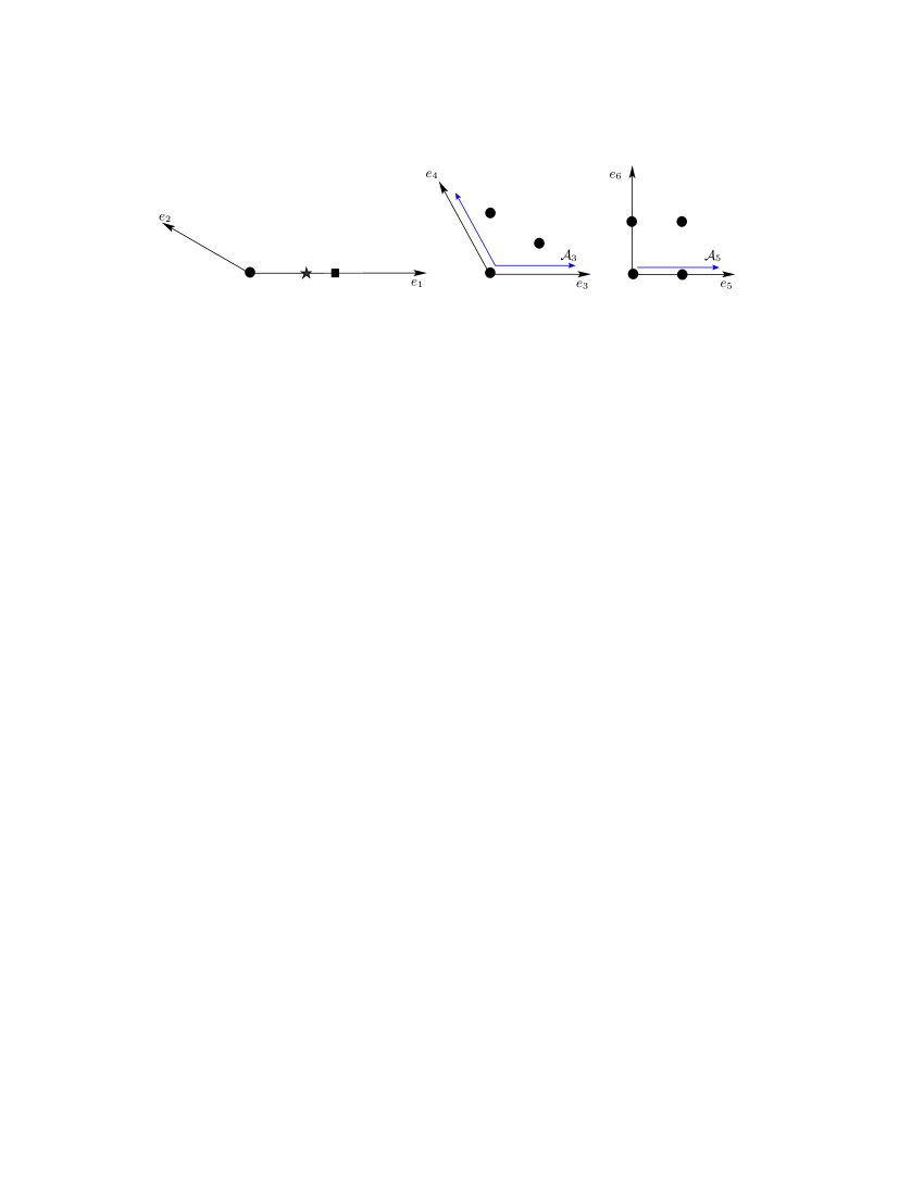
Figure 1: Geometry of the $T^{6}$ torus of a $\mathbbm{Z}_{6}$–II orbifold. The big dots denote points left invariant by $\vartheta$, the points denoted by a star and a square are fixed only under $\vartheta^{2}$ and $\vartheta^{3}$ respectively. In addition, the shorter/blue arrows denote the non-trivial Wilson lines given in Appendices A and B.

The twist for the $\mathbbm{Z}_{6}$–II orbifold is $v=\frac{1}{6}(0,\,1,\,2,\,-3)$, for which an admissible choice of $\Lambda$ is the root lattice of $G_{2}\times\mathrm{SU}(3)\times\mathrm{SO}(4)$ depicted in Figure 1. The action of the corresponding Coxeter element on the lattice basis is given by

$$\Theta e_{1}=2e_{1}+3e_{2}\,,\qquad\Theta e_{2}=-e_{1}-e_{2}\,,$$

$$\Theta e_{3}=e_{4}\,,\qquad\quad\qquad\Theta e_{4}=-e_{3}-e_{4}\,,$$

$$\Theta e_{5}=-e_{5}\,,\,\,\qquad\qquad\Theta e_{6}=-e_{6}\,.$$ (71)

Point group invariance of the metric, Eq. (17), implies that there are five free parameters (associated with three real Kähler moduli and one complex structure modulus). In total we have the following relations among the parameters (in string units, i.e. $R_{i}^{2}\equiv R^{2}_{i}/\alpha^{\prime}$)

$$R_{1}=\sqrt{3}\,R_{2}\,,\qquad R_{3}=R_{4}\,,\qquad\cos\varphi_{12}=-\frac{\sqrt{3}}{2}\,,\qquad\cos\varphi_{34}=-\frac{1}{2}$$ (72)

and the free parameters are $R_{1},\,R_{3},\,R_{5},\,R_{6},\,\cos\varphi_{56}$. Subsequently, using the standard definition of Kähler and complex structure moduli, Eq. (19), we find that the geometric parts of our moduli are given by

$$Re(T_{1})\equiv t_{1}=\frac{R_{1}^{2}}{4\sqrt{3}}\,,\quad Re(T_{2})\equiv t_{2}=\frac{\sqrt{3}}{4}\,R_{3}^{2}\,,\quad Re(T_{3})\equiv t_{3}=\frac{1}{2}R_{5}\,R_{6}\,\sin{\varphi_{56}}\,,$$

$$U_{3}\equiv u_{3}+\mathrm{i}\nu_{3}=\frac{R_{6}}{R_{5}}\,\sin{\varphi_{56}}+\mathrm{i}\,\frac{R_{6}}{R_{5}}\,\cos{\varphi_{56}}\,,$$ (73)

where $\varphi_{56}$ is the angle between $e_{5}$ and $e_{6}$.

The different models are obtained by choosing different gauge embeddings (i.e. different shift vectors and Wilson lines). We now present each in turn, and write down explicitly their low energy effective theories by applying the results of Section 3. We assume for simplicity that non-Abelian singlets acquire vevs as discussed in Subsection 3.6, which are constant $A_{\alpha}=\langle A_{\alpha}\rangle$ and of about the same order. Moreover, we assume that all the exotics and charged hidden matter are subsequently decoupled at the same scale, $M_{d}$. We then focus on the moduli and hidden gauge group only, since the observable matter must have vanishing expectation values in order to preserve the SM gauge group. Our dynamical fields are thus $S,T_{i},U_{3}$, $i=1,2,3$.

4.2.1 Model I: double gaugino condensate

The shift vector and Wilson lines for this model are given in Appendix A. The unbroken gauge group after compactification is $\mathrm{SU}(3)\times\mathrm{SU}(2)\times\mathrm{U}(1)_{Y}\times\left[\mathrm{SO}(8)\times\mathrm{SU}(3)\times\mathrm{U}(1)^{6}\right]$. The full 4D massless spectrum is given in Appendix  A.2. As explained above, the presence of discrete Wilson lines breaks the modular symmetry down to a congruence subgroup of $SL(2,\mathbb{Z})$. In the present model, we compute the modular symmetry group to be $SL(2,\mathbb{Z})\times\Gamma_{1}(3)\times\Gamma_{0}(4)\times\Gamma^{0}(4)$, where the transformations act on $T_{1},T_{2},T_{3}$ and $U$ respectively. We give some useful information about these groups in Appendix A.4. The resulting action is as follows.

Kähler potential.

The Kähler potential is given by (37), where the modular weights can be found in Table LABEL:tab:4DSpectrumModel and the Green-Schwarz coefficients are computed in Appendix A.7. They are

$$\delta_{GS}^{1}=-\tfrac{19}{3}\,,\quad\delta_{GS}^{2}=-\tfrac{7}{3}\,,\quad\delta_{GS}^{3}=0\,.$$ (74)

In principle, all the SM singlet vevs contribute to $K$. Since they must be small in order for us to maintain perturbative control, we can safely neglect them at this level.

Gauge kinetic function.

We can compute the gauge kinetic function by referring to Section 3.4.1. The values for the beta-function coefficients that measure the field theoretic threshold corrections turn out to be 

$$b_{SO(8)}=-9,\qquad\,b^{0}_{SO(8)}=-18$$ (75)

$$b_{SU(3)}=1,\qquad\quad b^{0}_{SU(3)}=-9\,.$$ (76)

Meanwhile, although stringy threshold corrections in the presence of discrete Wilson lines have been scarcely studied , we can infer their modular dependence from the modular symmetries and expected singularity structure. For example, assuming that the thresholds depend on $T_{2}$ as $\log[\eta(3\,T_{2})^{2}]$ leads to the required covariance under the modular symmetry $\Gamma_{1}(3)$ in the second plane, and reproduces the expected divergences as the volume of that plane goes to zero or infinity (see the paragraphs below Eq. (54)) . Moreover, as in the case without Wilson lines, we expect the contributing sectors to be the ${\mathcal{N}}=2$ ones, and this allows us to compute the coefficients of the thresholds. We study the corresponding auxiliary ${\mathcal{N}}=2$ theories in Appendix A.6.

Putting all information together, the final result for the two hidden gauge groups, $SO(8)$ and $SU(3)$, are respectively

$$f_{8} = S-\frac{9}{8\pi^{2}}\log{\frac{M_{d}}{M_{P}}}+\frac{2}{3\pi^{2}}\log\eta\left(3T_{2}\right)^{2}-\frac{1}{8\pi^{2}}\left(\log\eta\left(4T_{3}\right)^{2}+\log\eta\left(U/4\right)^{2}\right)\,,$$ (77)

$$f_{3} = S-\frac{5}{4\pi^{2}}\log{\frac{M_{d}}{M_{P}}}-\frac{1}{12\pi^{2}}\log\eta\left(3T_{2}\right)^{2}-\frac{3}{8\pi^{2}}\left(\log\eta\left(4T_{3}\right)^{2}+\log\eta\left(U/4\right)^{2}\right)\,.$$ (78)

At this point one can check explicitly, using the data in the Appendix A.2, that the constraint (64) is indeed satisfied, and the expressions are modular covariant. Another nice check of the threshold coefficients is to note that computations for all the gauge groups lead to the same Green-Schwarz anomaly coefficients for the sigma-model and modular anomalies, via Eq. (55).

Superpotential.

The superpotential for the moduli receives contributions from Yukawa couplings, higher order matter couplings and gaugino condensation. In the moduli potential, we neglect the higher order couplings, since they will be suppressed with respect to the trilinear Yukawa couplings by the Planck scale and the small matter vevs (see however [51]). Also, we consider only couplings between (non-Abelian) singlets, since we allow non-trivial vevs only for those fields.

The allowed Yukawa couplings are computed in Appendix A.3. All those between gauge singlets are of the kind $\vartheta^{2}\vartheta^{5}\vartheta^{5}$. From (38)-(23), we can explicitly compute this coupling in terms of the $T_{i}$ moduli (see Appendix C for details). The result is:

$$Y^{25}_{\alpha\beta\gamma}=F_{\alpha\beta\gamma}\,g_{s}\sqrt{t_{1}t_{2}}\,N_{255}\sum_{u_{1},u_{2}}\exp{(-{\it b}_{u_{1}}\,T_{1}-{\it b}_{u_{2}}\,T_{2})}\,,$$ (79)

where

$$N_{255}=\frac{2^{14/3}\pi^{4}}{3^{3/2}\Gamma^{6}(1/3)}\,,$$ (80)

$${\it b}_{u_{1}}=\pi u_{1}^{t}\,L_{1}\,u_{1}\,,\qquad{\it b}_{u_{2}}=\pi u_{2}^{t}\,L_{2}\,u_{2}\,,$$ (81)

$$L_{1}=\left(\begin{array}[]{ccc}6&&-3\\ -3&&2\end{array}\right)\,,\qquad\qquad L_{2}=\left(\begin{array}[]{ccc}2&&-1\\ -1&&2\end{array}\right)\,.$$ (86)

The 2D lattice vectors $u_{i}$ depend on the fixed points $(f_{\alpha},\,f_{\beta},\,f_{\gamma})$ of the fields involved in the coupling, and are given in C.2, as are the normalisation factors $F_{\alpha\beta\gamma}$.

The corresponding contributions to the holomorphic superpotential are computed using (79) and (44). In Appendix C.3 we explain the necessary tricks to show that the explicit expressions are modular covariant, as they must be. Here, we consider only the leading order terms in the sum over instantons, and replace the SM singlets by their vevs $A_{\alpha}$. The result is 

$$W_{\it yuk}=2\,N_{255}\,A_{1}^{2}\,e^{-2\pi\,T_{2}/3}\left(A_{2}+A_{3}e^{-2\pi\,T_{1}/3}\right)\,.$$ (87)

Finally, with the gauge kinetic functions in hand, we can immediately write down the contribution to the superpotential that arises when the gauginos in the hidden sector condense:

$$W_{\it gc}=-\frac{c}{e}\,\frac{3}{16\pi^{2}}\,\,e^{-4\pi^{2}S/3}\,\left(\frac{M_{d}}{M_{P}}\right)^{3/2}\,\eta(3\,T_{2})^{-16/9}\,\left[\eta(4\,T_{3})\,\eta(U/4)\right]^{1/3}$$

$$\hskip 56.9055pt-\frac{c}{e}\,\frac{3}{32\pi^{2}}\,e^{-8\pi^{2}S/3}\,\left(\frac{M_{d}}{M_{P}}\right)^{10/3}\,\eta(3\,T_{2})^{4/9}\,\,\left[\eta(4\,T_{3})\,\eta(U/4)\right]^{2}\,,$$ (88)

where we have used the definition of $d_{a}$ in (62). Notice here that several of the Dedekind eta functions, originating from the stringy threshold corrections, appear with positive powers, in contrast to what is usually assumed in the literature. We comment below on the implications of this for moduli stabilisation.

Before looking at the moduli stabilisation and de Sitter vacua, we present a second representative model, which has a single hidden sector gauge group.

4.2.2 Model II: single gaugino condensate

The shift vector, Wilson lines, massless spectrum and all other details of this model are given in Appendix B. The unbroken gauge group after compactification is $\mathrm{SU}(3)\times\mathrm{SU}(2)\times\mathrm{U}(1)_{Y}\times\left[\mathrm{SO}(14)\times\mathrm{U}(1)^{5}\right]$. The modular symmetry is broken by the Wilson lines to $SL(2,\mathbb{Z})\times\Gamma_{1}(3)\times\Gamma_{1}(2)\times\Gamma^{1}(2)$, where the transformations act on $T_{1},T_{2},T_{3}$ and $U$ respectively.

The computation of the action follows exactly as for Model I, and again we relegate the details to the appendix.

Kähler potential.

The Kähler potential is given by (37), where the modular weights can be found in Table LABEL:tab:4DSpectrumModel2, and the Green-Schwarz coefficients are

$$\delta_{GS}^{1}=-11\,,\quad\delta_{GS}^{2}=-\frac{11}{3}\,,\quad\delta_{GS}^{3}=0\,.$$ (89)

Again, we neglect contributions to $K$ from the singlet vevs, since they are small.

Gauge kinetic function.

The beta-function coefficients that measure the field theoretic threshold corrections are

$$b_{SO(14)}=-29,\qquad\,b^{0}_{SO(14)}=-36\,.$$ (90)

Thus, the gauge kinetic function for the single hidden sector is given by

$$f_{14}=S-\frac{7}{8\pi^{2}}\log{\frac{M_{d}}{M_{P}}}+\frac{7}{6\pi^{2}}\,\log\eta\left(3\,T_{2}\right)^{2}+\frac{5}{8\pi^{2}}\left(\log\eta\left(2\,T_{3}\right)^{2}+\log\eta\left(U/2\right)^{2}\right)\,.$$ (91)

Using the data in Appendix B, we can check that the constraint (64) is satisfied, the expressions are modular covariant, and the universal $\delta_{GS}^{j}$ are obtained.

Superpotential.

As in the previous model, we consider the contributions to the superpotential from Yukawa couplings and gaugino condensation. The allowed Yukawa couplings for this model are computed in Appendix B. As before, couplings among singlets are all between $\vartheta^{2}\vartheta^{5}\vartheta^{5}$ sectors, and the expressions for the couplings in terms of the $T_{i}$ moduli can be found in Appendix C. Using the notation in the appendix, we can have couplings of four types.

We can compute the holomorphic superpotential and check that the expressions are modular covariant. In what follows, we consider only the following terms 

$$W_{\it yuk}=2\,N_{255}\,A_{1}^{2}\,\left(A_{2}+A_{3}\,e^{-2\pi\,T_{1}/3}\right)\,,$$ (92)

where we have considered only the leading instanton contributions, and replaced the singlets by their vevs. Notice the important fact that a constant piece has naturally arisen, coming from the leading contribution to the Yukawa coupling between twisted fields localised at the same fixed point (see Appendix C.2).

Finally, the gaugino condensation contribution to the superpotential is simply,

$$W_{\it gc}=-\frac{c}{e}\,\frac{3}{8\pi^{2}}\,\,e^{-2\pi^{2}S/3}\,\left(\frac{M_{d}}{M_{P}}\right)^{7/12}\,\eta(3\,T_{2})^{-14/9}\,\left[\eta(2\,T_{3})\,\eta(U/2)\right]^{-5/6}\,.$$ (93)

Notice that in this case, the Dedekind eta functions do appear with negative powers in the superpotential, as is usually assumed.

4.3 Towards stabilisation of moduli and de Sitter vacua

In this section, we study the problem of moduli stabilisation and de Sitter vacua in the two explicit orbifold models discussed in the previous section.

The scalar potential that governs the dynamics of the moduli, after having integrated out the hidden matter, is given to a good approximation (in Planck units) by

$$V_{F}=e^{K}\,|W|^{2}\Bigg{[}\left|Y\,\frac{W_{S}}{W}-1\right|^{2}+\sum_{j}\frac{Y}{Y-\delta^{j}}\,\left|\delta^{j}\,\,\frac{W_{S}}{W}+(\phi_{j}+\bar{\phi_{j}})\,\frac{W_{\phi_{j}}}{W}-1\right|^{2}-3\,\,\Bigg{]}\,,$$ (94)

where, as before, $Y=S+\bar{S}-\sum_{j}\delta^{j}\,\log{(\phi_{j}+\bar{\phi_{j}})}$ with $\phi_{j}=T_{1},T_{2},T_{3},U$, $\delta^{j}=\frac{\delta_{GS}^{j}}{8\pi^{2}}$, and now $W=W_{yuk}+W_{gc}$. We have to analyse this potential for the five complex fields $S,T_{1},T_{2},T_{3}$ and $U$. Due to the complexity of the system, we can only make limited progress analytically, in particular we can solve for the axionic parts. Thereafter, our search for vacua will be numerical. First, however, we can make some general observations.

4.3.1 de Sitter vacua

Before considering the moduli stabilisation mechanisms that may be at work, let us begin by discussing the structure of the potential, and in particular the possibility of obtaining de Sitter solutions. From (94) we see that the positivity of the potential depends basically on how large the ratios $W_{a}/W$ can be, compared to one. If three of our five fields have $W_{a}/W$ sufficiently smaller or larger than one, then the potential will certainly be positive. In order for it to be negative, the ratio $W_{a}/W$ has to be of order one for at least three of the fields. One can then analyse the dependence of the ratio $W_{a}/W$ for each field. For this, let us recall the orders of magnitude that we are considering. i) The vevs of the matter fields must be around $A_{\alpha}\lesssim 10^{-1}$ in order for the calculation of the Kähler potential to be valid. ii) The decoupling scale must be lower than the Planck scale and thus we have $M_{d}\lesssim 10^{-1}M_{P}$.

For Model II, it is simple to estimate that the contribution from the dilaton will generically give rise to a constant bigger than one, and thus can cancel a big part of the negative piece in the potential. Moreover, for $T_{1}$, the ratio $W_{a}/W$ can be seen to be much less than one, thus contributing again to the positivity of $V$. For the other fields, it depends on $\eta^{\prime}$ and thus can in principle be of order one and therefore give a null contribution to the potential. The upshot is that for Model II we can generically expect $V>0$, and thus, de Sitter vacua. An analogous analysis can be made for Model I, with similar results. Note that the loop contribution from $\delta^{j}$ is always smaller than the others, as it must be.

We now ask whether or not we can expect to find vacua with all the moduli stabilised.

4.3.2 The modular form mechanism for $T_{2},T_{3},U$

Let us first focus on the three moduli, $T_{2},T_{3},U$, which appear in the superpotential due to stringy threshold corrections, via the Dedekind eta functions defined in (30). It was suggested in [20] that such a dependence may be enough to force compactification and moduli stabilisation. In particular, if the eta functions appear in the superpotential with negative powers, then the scalar potential diverges as the relevant moduli go to zero and infinity (this can be seen by recalling the asymptotic behaviour of the eta function described in Section 3.1). Then a minimum in these directions is guaranteed. Moreover, with the simplest factorisable superpotentials such as those corresponding to a single gaugino condensate only, the fixed points under the modular transformations are necessarily extrema of the potential [20, 22].

Although the latter property is not observed for our models, which have more complicated superpotentials, Model II does have the required asymptotic behaviour to ensure the existence of minima in the $T_{2},T_{3},U$ directions. However, in Model I, which is also a very common one in the landscape, the Dedekind eta functions appear in the superpotential with positive powers, so that the scalar potential goes to zero as the relevant moduli go to zero and infinity. In that case, we cannot ensure the existence of minima. Notice also that in realistic orbifolds like the ones we consider here, Wilson lines break the modular symmetries in each plane in different ways, and thus generically, it is not correct to assume equality of all the Kähler moduli (the dependence of the superpotential on each Kähler modulus assumes a different functional form).

The existence of multiple gaugino condensates and how the threshold corrections enter the superpotential are somehow correlated with each other. If the $E_{8}\times E_{8}$ gauge group is broken down to yield multiple non-Abelian hidden gauge groups, the latter will tend to be small, and thus one can expect to find large amounts of hidden matter. At the same time, much hidden matter, whether massless or massive, drives the auxiliary ${\mathcal{N}}=2$ beta-function coefficients towards positive values, which in turn means that the eta functions appear with positive powers in $W_{gc}$.

The case of $T_{2}$ in Model I is slightly different since it also always appear in the Yukawa couplings. Thus a different mechanism may help to stabilise this field.

4.3.3 Racetrack and KKLT for $\boldsymbol{S,T_{1},T_{2}}$

The dependence of the potential on $T_{1}$ can occur only via the non-perturbative Yukawa couplings in $\mathbbm{Z}_{6}$-II orbifolds. The form of the superpotential is then reminiscent of the KKLT one [16], albeit with coefficients that depend on the other moduli. The same is true for $S$, in the case of a single gaugino condensate. Otherwise, $S$ may be stabilised with a racetrack induced by multiple gaugino condensates (see [15]). Similarly, if $T_{2}$ appears in $W_{yuk}$, it may have a racetrack behaviour, with $W_{yuk}$ competing against the leading dependence in $W_{gc}$.

Since the standard racetrack and KKLT stabilisation mechanisms both require some degree of tuning of the coefficients, and since in our case those coefficients are actually field-dependent, whether or not they are successful in producing a minimum in all directions must be studied explicitly. We now turn to that analysis.

4.3.4 Stabilisation of the axions

We can make significant progress by first considering the imaginary parts of our five complex fields, the axions. These turn out to have periodic potentials, with multiple minima and maxima, several of which can be found analytically. To begin with, recall that the axions contribute to the scalar potential only via the superpotential.

For the axions entering the potential via the Dedekind eta functions, it is in general difficult to identify the positions of all the extrema. For example, only for the simplest superpotentials do the fixed points correspond to extrema. However, it turns out that ${\rm Im}\,\phi_{j}=0$ are typically minima, and so we may choose those points. This simplifies the problem for the remaining fields . For example, consider the superpotential for Model II, which can now be written in the form

$$W=C_{1}\,e^{-c_{1}T_{1}}+C_{2}(T_{2},T_{3},U)\,e^{-c_{2}S}+C_{3}$$ (95)

with all the coefficients real. This is reminiscent of a KKLT superpotential [16] for the fields $T_{1}$ and $S$, although here the KKLT coefficients are no longer constants, but depend on the other fields. For the dependence on $T_{2},T_{3}$ and $U$, let us consider just the leading terms in the eta functions. Then the superpotential is simply a sum of exponentials, and the derivatives that appear in the scalar potential are easy to compute.

Similar to the basic KKLT model, the resulting scalar potential depends on ${\rm Im}\,T_{1}=\sigma_{1}$ and ${\rm Im}\,S=\sigma_{S}$ as terms proportional to $\cos c_{1}\sigma_{1}$, $\cos c_{2}\sigma_{S}$ and $\cos(c_{1}\sigma_{1}-c_{2}\sigma_{S})$. The magnitudes and signs of the coefficients depend on $C_{1},C_{2},C_{3}$ as well as the real parts of the five complex fields. In any case, it is clear that $\sigma_{1}=n_{1}\pi/c_{1}$ and $\sigma_{S}=n_{2}\pi/c_{2}$, with $n_{1},n_{2}$ integers, are critical points, and so they represent interesting candidates for the minima. Notice that analogous arguments can be made for models that fall into the racetrack class.

With extrema for the five imaginary parts in hand, we now turn to a numerical analysis for the real parts. We have also scanned numerically for all ten real and imaginary parts together.

4.3.5 Numerical results and explicit dS vacua

We have tried several methods to search numerically for minima in the scalar potential . The most successful one we found was to search for solutions to the critical point equations  $\partial V/\partial x^{A}=0$ for $x^{A}$ the real (and imaginary) parts of $S,T_{i},U$.

By varying the input parameters $c,A_{\alpha}$ and $M_{d}$ we have identified several critical points consistent with our approximations  in both models. In Tables 1 and 2 we show some representative vacua of Model I and Model II, respectively. Mathematica codes with all the details of these vacua can be found at our webpage [52].

Parameters
$c=1/10$	$20A_{1}=100A_{2}=A_{3}=1/10$	$M_{d}=1/65$
Moduli vevs
$\phi_{i}$	${\rm Re}\langle\phi_{i}\rangle$	${\rm Im}\langle\phi_{i}\rangle$
$T_{1}$	$3.51166$	$3/2$
$T_{2}$	$0.24201$	$-1/3$
$T_{3}$	$7.05981$	$35/8$
$U$	$112.95695$	$-506$
$S$	$0.09385$	$1079/144\pi$
Cosmological constant $\Lambda=6.45\times 10^{-19}$
Effective dilaton $Y=0.32262$
Mass eigenstates
$\rho_{i}\sim\phi_{i}$	$m^{2}_{{\rm Re}\rho_{i}}$	$m^{2}_{{\rm Im}\rho_{i}}$
$\rho_{1}$	$1.87\times 10^{-18}$	$3.57\times 10^{-18}$
$\rho_{2}$	$-4.76\times 10^{-17}$	$1.2\times 10^{-17}$
$\rho_{3}$	$3.15\times 10^{-20}$	$3.29\times 10^{-33}$
$\rho_{U}$	$9.84\times 10^{-23}$	$1.51\times 10^{-94}$
$\rho_{S}$	$1.14\times 10^{-16}$	$2.16\times 10^{-16}$
Tachyon: ${\rm Re}\rho_{2}\sim 0.9{\rm Re}T_{2}+0.4{\rm Re}S$

Table 1: An unstable de Sitter solution of Model I. The dominant contribution to the mass eigenstate $\rho_{i}$ arises from the modulus $\phi_{i}$. In particular, the tachyon is dominated by the ${\rm Re}\,T_{2}$ direction, as can also be appreciated in Figure 2. We give the solution to 5 significant figures, but we have computed it to a precision of 1000. The value of $\Lambda$ is given in Planck units.

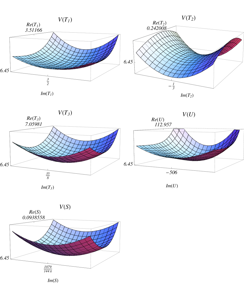
Figure 2: Scalar potental as a function of the bulk moduli of Model I for the vacuum presented in Table 1. The scalar potential is rescaled by a factor $10^{19}$.

Parameters
$c=1/2$	$A_{1},A_{2},A_{3}=1/2$	$M_{d}=1/600$	$c=1/200$	$A_{1},A_{2},A_{3}=1/2$	$M_{d}=10^{-3}$
Moduli vevs
$\phi_{i}$	${\rm Re}\langle\phi_{i}\rangle$	${\rm Im}\langle\phi_{i}\rangle$	$\phi_{i}$	${\rm Re}\langle\phi_{i}\rangle$	${\rm Im}\langle\phi_{i}\rangle$
$T_{1}$	$0.60565$	$3/2$	$T_{1}$	$0.60213$	$3/2$
$T_{2}$	$2.05917$	$19/6$	$T_{2}$	$3.99948$	$19/6$
$T_{3}$	$6.48601$	$37/4$	$T_{3}$	$11.95957$	$37/4$
$U$	$25.94402$	$-3$	$U$	$47.83828$	$-3$
$S$	$0.53034$	$809/144\pi$	$S$	$0.97758$	$809/144\pi$
Cosmological constant $\Lambda=7.41\times 10^{-6}$			$\Lambda=5.12\times 10^{-7}$
Effective dilaton $Y=1.15312$			$Y=2.07762$
Mass eigenstates
$\rho_{i}\sim\phi_{i}$	$m^{2}_{{\rm Re}\rho_{i}}$	$m^{2}_{{\rm Im}\rho_{i}}$	$\rho_{i}\sim\phi_{i}$	$m^{2}_{{\rm Re}\rho_{i}}$	$m^{2}_{{\rm Im}\rho_{i}}$
$\rho_{1}$	$2.88\times 10^{-5}$	$2.28\times 10^{-4}$	$\rho_{1}$	$2.57\times 10^{-6}$	$2.02\times 10^{-5}$
$\rho_{2}$	$-1.67\times 10^{-5}$	$8.34\times 10^{-19}$	$\rho_{2}$	$-1.92\times 10^{-7}$	$8.61\times 10^{-36}$
$\rho_{3}$	$5.57\times 10^{-7}$	$1.21\times 10^{-37}$	$\rho_{3}$	$1.2\times 10^{-8}$	$1.23\times 10^{-68}$
$\rho_{U}$	$2.84\times 10^{-8}$	$7.57\times 10^{-39}$	$\rho_{U}$	$5.97\times 10^{-10}$	$7.72\times 10^{-70}$
$\rho_{S}$	$4.27\times 10^{-4}$	$7.87\times 10^{-4}$	$\rho_{S}$	$5.28\times 10^{-5}$	$6.72\times 10^{-5}$
Tachyon: ${\rm Re}\rho_{2}\sim 0.9{\rm Re}T_{2}+0.3{\rm Re}T_{3}+0.4{\rm Re}S$			${\rm Re}\rho_{2}\sim 0.9{\rm Re}T_{2}+0.4{\rm Re}T_{3}+0.2{\rm Re}S$

Table 2: Unstable de Sitter solutions to Model II. As in Model I, the dominant contribution to the tachyon arises from ${\rm Re}T_{2}$. The potential $V({\rm Re}T_{2})$ differs from the one for Model I because the tachyon has some components in some other real directions. A change in the input parameters provides a larger value for $Y$. We give the solution to 5 significant figures, but we have computed it to a precision of 1000.

The vacua we find are all de Sitter, however they all turn out to have at least one unstable direction in the moduli space. This is evident from the plot of the scalar potential as a function of ${\rm Re}\,T_{2}$ in Model I, and/or from the mass eigenvalues, displayed in Tables 1 and 2. One might be tempted to think that a shift to the left in $V({\rm Re}\,T_{2})$ of Model I leads to the true minimum. However, this is not sufficient since any change in ${\rm Re}\,T_{2}$ affects the whole scalar potential, resulting in a vacuum with (more) instabilities in other directions. In general, we have found it very difficult to avoid instabilities in the direction ${\rm Re}\,(T_{2},\,T_{3},\,U)$. It would be important to understand the reason for these instabilities, and whether or not they are inevitable.

An interesting feature of both models is that there are some almost flat directions, as observed from the hierarchically small masses. The corresponding eigenvectors are linear combinations of ${\rm Im}\,S,{\rm Im}\,T_{3}$ and ${\rm Im}\,U$ (and also ${\rm Im}\,T_{2}$ for Model II). The reason for these almost flat directions is as follows. First, notice that in Model I, the contribution to $W_{gc}$ from the $\mathrm{SU}(3)$ gaugino condensate is typically highly suppressed with respect to the $\mathrm{SO}(8)$ condensate due to the stronger exponential suppression in $S$, and the stronger suppression in $M_{d}/M_{P}$. Thus, effectively, we have only a single condensate in both models. Moreover, the higher order contributions to the eta functions in both Model I and Model II, at their solutions, are strongly suppressed for $T_{3}$ and $U$ (the same can be said for $T_{2}$, when ${\rm Re}\,T_{2}$ becomes larger than one as in Model II). Therefore, to a good approximation, ${\rm Im}\,S,{\rm Im}\,T_{3}$ and ${\rm Im}\,U$ (and ${{\rm Im}\,T_{2}}$ for Model II) appear in the superpotential, and thus in the scalar potential, only via a single linear combination, which, e.g. for Model I, can be written as

$$X~{}=~{}-\frac{4\pi^{2}}{3}{\rm Im}\,S-\frac{\pi}{9}{\rm Im}\,T_{3}-\frac{\pi}{144}{\rm Im}\,U\,.$$ (96)

As a consequence, to a good approximation, only this linear combination of the three (or four) fields is lifted by the non-perturbative dynamics, leaving two (or three) linearly independent combinations as flat directions, and two (or three) corresponding shift symmetries. Of course, the higher order corrections do lift the latter directions, rendering them only almost flat. We expect this feature to be also present in any metastable minima that may exist, being quite a generic consequence of the moduli stabilisation via gaugino condensation with threshold corrections. Such almost flat directions could potentially be interesting, since extremely light scalar fields are often called upon in cosmological models, for inflation, quintessence and the like.

Finally, we comment on the vevs of the moduli that we find. Of course, due to the instabilities, our vacua cannot be considered as candidates for our universe, and so we have not attempted to obtain realistic values for the moduli at this stage. However, consistency of our analysis does impose some constraints. In particular, the overall volume must be large enough for the supergravity approximation to hold, and the dilaton large enough for the string loop expansion to be a good one. The latter is difficult to achieve, as has long been known in heterotic orbifolds. Meanwhile, it is interesting that anistropic compactifications emerge quite naturally in our setup, since these have been proposed to explain the mild hierarchy between the GUT and string scales.

5 Discussion

We have revisited the problem of moduli stabilisation in heterotic orbifold compactifications, in the light of the recent discovery of fertile patches in the heterotic landscape where the MSSM spectrum can be found. After reviewing the derivation of the low energy effective action describing general orbifold compactifications, we computed it explicitly for two concrete MSSM models. Our resulting actions survived several non-trivial checks, such as modular invariance, including a new stringy constraint on the matter content in the presence of gaugino condensation (64). Finally, we studied the dynamics for all the bulk moduli fields, making use of numerical techniques. We found several de Sitter vacua, but unfortunately they all suffer from instabilities. Curiously, we did not uncover any anti-de Sitter vacua that were consistent with our assumptions. Since the scalar potential grows rapidly, we expect them to appear at very small moduli vevs, which are not consistent with our approximations. On the other hand, the values of the cosmological constant at the vacua tend to be very large, although we should recall that this is counting only the classical value for the vacuum energy.

Given that we have found it difficult to locate metastable vacua, it is interesting to compare our results with previous toy models for heterotic orbifold compactifications. The most recent of these is [18], which treated two bulk moduli, $S$ and $T$, together with a complex matter field. Although they included a D-term contribution, it turns out to be vanishingly small, so that their setup is very similar to ours. Indeed, it is easy to find metastable minima to their F-term potential. Thus it seems that the challenge we meet comes from considering all five bulk moduli fields that are present and the comparatively small number of free parameters.

Our analysis leads us to question if new ingredients, beyond those already considered in the literature, may well be necessary in order to stabilise all the moduli. Along those lines, recall that we have neglected some moduli-dependent contributions to the effective Lagrangian, which are known to be present, but have been little studied. Firstly, there is a universal contribution to the threshold corrections [41], and secondly an overall factor in the Yukawa couplings, which can depend on bulk moduli of the untwisted planes [37]. It would also be very useful to have in hand direct and explicit computations of the threshold corrections in the presence of discrete Wilson lines [50]. Other effects that depend on the moduli and merit further study are those arising from the Casimir Energy and Coleman-Weinberg potential, which become relevant after supersymmetry breaking (see e.g. [53]).

Otherwise, the main unknown in our analysis has been the dynamics that decouples exotics and hidden matter, which we parametrised with some (non-Abelian) singlet vevs and the decoupling mass scale. The introduction of this high scale, which separates the dynamics of the matter and moduli, is important for several reasons. Phenomenologically, we know that the exotics must be decoupled at least at the GUT scale to maintain gauge coupling unification, and yet the gauge hierarchy problem suggests supersymmetry breaking should occur down at the TeV scale. Practically, it renders the system tractable; indeed already with 10 real bulk moduli the search for minima has proven to be a significant challenge. Occasionally, it is also important because hidden matter, if not massive, tends to destroy asymptotic freedom in the hidden gauge groups, preventing the gauginos from condensing there.

We remark that in considering only the bulk moduli stabilisation, we have assumed that all the other flat directions, corresponding to twisted fields, may be lifted in the decoupling process, and this certainly deserves more attention. One can argue that, since the orbifold MSSM candidates arise from ${\mathcal{N}}=(0,2)$ models, the massless twisted fields might not generically correspond to blow-up modes [4]; thus it should be possible to stabilise them and remain within the orbifold description where we have much more control. A detailed treatment of the decoupling dynamics would require, among other things, explicit computations of the higher order couplings between non-Abelian singlet fields, and non-Abelian singlets and charged matter. For progress in this direction see [40]. Notice that if a decoupling scale is in play, D-term potentials are no longer relevant for the bulk moduli dynamics, since all the $\mathrm{U}(1)$ gauge groups are broken when the non-Abelian singlets acquire vevs (all the non-Abelian singlets are generically charged under all the hidden $\mathrm{U}(1)$’s).

Although unstable, the dS vacua we have found do have some interesting properties. In particular, the non-perturbative dynamics (i.e. gaugino condensation with threshold corrections) tends to give rise to some almost flat directions, and consequently hierarchically light fields. We expect that this feature can also hold for any metastable dS vacua that might exist. Light fields could be useful for cosmology, and it would then be important to understand how quantum corrections contribute to the light masses after supersymmetry breaking.

So far we must say that our results on the (non-)existence of metastable de Sitter in MSSM heterotic orbifolds are inconclusive. We are now developing more sophisticated numerical codes to scan our scalar potentials for metastable minima, and are widening our search in the minilandscape of MSSM models [48]. Then we must also ask if a model can be found with realistic values for the moduli vevs, including Re $S\sim 2$, an appropriate gravitino mass and cosmological constant. If and when such a vacuum is found, it would have a host of applications. We could begin to study in detail the phenomenological and cosmological aspects of the compactification, starting with supersymmetry breaking and the low energy sparticle spectrum, models of inflation, resolutions to the cosmological moduli problem and so on.

Appendix A Details of Model I

In this appendix we describe in detail our first explicit MSSM orbifold compactification. We specify the orbifold, and present its complete 4D massless spectrum, along with the trilinear couplings allowed by the standard selection rules. Then we describe the modular symmetries and anomalies, and compute the coefficients that measure the stringy threshold corrections to the gauge kinetic functions.

A.1 Model definition

The model is defined by the following shift vector and Wilson lines

$$V^{\text{SO(10),1}} = \left(\tfrac{1}{3},\,-\tfrac{1}{2},\,-\tfrac{1}{2},\,0,\,0,\,0,\,0,\,0\,\right)\left(\tfrac{1}{2},\,-\tfrac{1}{6},\,-\tfrac{1}{2},\,-\tfrac{1}{2},\,-\tfrac{1}{2},\,-\tfrac{1}{2},\,-\tfrac{1}{2},\,\tfrac{1}{2}\,\right)\,,$$ (97)

$${\cal A}_{5} = \left(0,\,\tfrac{1}{2},\,\tfrac{1}{2},\,\tfrac{1}{2},\,-\tfrac{1}{2},\,0,\,0,\,0\,\right)\left(1,\,0,\,0,\,0,\,2,\,-2,\,0,\,0\,\right)\,,$$

$${\cal A}_{3} = \left(0,\,-1,\,-\tfrac{1}{3},\,-\tfrac{1}{3},\,-\tfrac{1}{3},\,-\tfrac{1}{3},\,-\tfrac{1}{3},\,\tfrac{2}{3}\,\right)\left(\tfrac{10}{3},\,-2,\,-4,\,-\tfrac{7}{3},\,-\tfrac{7}{3},\,-4,\,-3,\,3\,\right)\,.$$

The Wilson lines ${\cal A}_{3}$ (order 3) and ${\cal A}_{5}$ (order 2) lift the degeneracy of the fixed points in the second and third torus, respectively. A possible second order 2 Wilson line in the third torus is set to zero. The 4D gauge group after compactification is

$$\mathrm{SU}(3)_{C}\times\mathrm{SU}(2)_{L}\times\mathrm{U}(1)_{Y}\times\left[\mathrm{SO}(8)\times\mathrm{SU}(3)\times\mathrm{U}(1)^{6}\right]\,.$$ (98)

The $\mathrm{U}(1)$ generators are chosen to be

$$t_{1} = t_{\rm X}=\left(\tfrac{5}{3},\,1,\,-\tfrac{5}{3},\,\tfrac{1}{3},\,\tfrac{1}{3},\,\tfrac{1}{3},\,\tfrac{1}{3},\,\tfrac{1}{3}\,\right)\left(-\tfrac{1}{3},\,-\tfrac{7}{3},\,0,\,\tfrac{1}{3},\,\tfrac{1}{3},\,0,\,0,\,0\,\right)\,,$$ (99a)

$$t_{2} = t_{\rm Y}=\left(0,\,0,\,0,\,\tfrac{1}{2},\,\tfrac{1}{2},\,-\tfrac{1}{3},\,-\tfrac{1}{3},\,-\tfrac{1}{3}\,\right)\left(0,\,0,\,0,\,0,\,0,\,0,\,0,\,0\,\right)\,,$$ (99b)

$$t_{3} = \left(-45,\,321,\,45,\,-9,\,-9,\,-9,\,-9,\,-9\,\right)\left(9,\,63,\,0,\,-9,\,-9,\,0,\,0,\,0\,\right)\,,$$ (99c)

$$t_{4} = \left(246,\,0,\,75,\,-15,\,-15,\,-15,\,-15,\,-15\,\right)\left(15,\,105,\,0,\,-15,\,-15,\,0,\,0,\,0\,\right)\,,$$ (99d)

$$t_{5} = \left(0,\,0,\,171,\,15,\,15,\,15,\,15,\,15\,\right)\left(-15,\,-105,\,0,\,15,\,15,\,0,\,0,\,0\,\right)\,,$$ (99e)

$$t_{6} = \left(0,\,0,\,0,\,3,\,3,\,3,\,3,\,3\,\right)\left(54,\,-21,\,0,\,-54,\,-54,\,0,\,0,\,0\,\right)\,,$$ (99f)

$$t_{7} = \left(0,\,0,\,0,\,21,\,21,\,21,\,21,\,21\,\right)\left(0,\,15,\,0,\,0,\,0,\,0,\,0,\,0\,\right)\,,$$ (99g)

where $t_{Y}$ and $t_{X}$ denote respectively the hypercharge and the anomalous $\mathrm{U}(1)$ generator.

A.2 4D spectrum

The spectrum in the untwisted sector includes: the graviton, the axio-dilaton, $S$, the gauge bosons of the gauge group (98), the Kähler moduli $T_{i}$, $i=1,2,3$, the complex structure modulus $U_{3}$ (cf. Section 4.2), and their corresponding supersymmetric partners. In addition, the spectrum contains the matter fields with non-zero quantum numbers given in Table LABEL:tab:4DSpectrumModel. They amount to three generations of quarks and leptons plus vector-like exotics with respect to $\mathcal{G}_{\mathrm{SM}}$ and hidden matter.

Table 3: The spectrum of the $\mathbbm{Z}_{6}$–II Model I. We denote the fixed points, $f$, in the $\vartheta^{k}$ (un)twisted sector, with their (real) lattice coordinates. A pair of coordinates $(-,-)$ indicates that the corresponding torus is left fixed in the sector. We give the representations under $SU(3)_{C}\times SU(2)_{L}\times SO(8)\times SU(3)$ respectively, and the $\mathrm{U}(1)$ charges $q_{i}$ with respect to the basis of generators given above. $n^{i}$ and $\ell^{i}$ are the Kähler and complex structure modular weights in the $i$th torus.

$f$	Repr.	$q_{\mathrm{X}}$	$q_{Y}$	$q_{3}$	$q_{4}$	$q_{5}$	$q_{6}$	$q_{7}$	$n^{1}$	$n^{2}$	$n^{3}$	$\ell^{3}$	Label​​
$\vartheta^{0}$ sector
	$(\boldsymbol{1},\boldsymbol{1},\boldsymbol{1},\boldsymbol{1})$	$-\frac{4}{3}$	$0$	$-138$	$-123$	$123$	$\frac{15}{2}$	$\frac{105}{2}$	$-1$	$0$	$0$	$0$	$n_{1}$
	$(\boldsymbol{1},\boldsymbol{1},\boldsymbol{1},\boldsymbol{1})$	$\frac{2}{3}$	$-1$	$156$	$-168$	$-78$	$\frac{3}{2}$	$\frac{21}{2}$	$-1$	$0$	$0$	$0$	$\overline{e}_{1}$
	$(\boldsymbol{\overline{3}},\boldsymbol{1},\boldsymbol{1},\boldsymbol{1})$	$\frac{2}{3}$	$\frac{2}{3}$	$156$	$-168$	$-78$	$\frac{3}{2}$	$\frac{21}{2}$	$-1$	$0$	$0$	$0$	$\bar{u}_{1}$
	$(\boldsymbol{1},\boldsymbol{1},\boldsymbol{8},\boldsymbol{1})$	$\frac{7}{3}$	$0$	$-63$	$-105$	$105$	$21$	$-15$	$0$	$-1$	$0$	$0$	$\widetilde{N}_{2}$
	$(\boldsymbol{3},\boldsymbol{2},\boldsymbol{1},\boldsymbol{1})$	$\frac{4}{3}$	$-\frac{1}{6}$	$-210$	$78$	$-78$	$\frac{3}{2}$	$\frac{21}{2}$	$0$	$-1$	$0$	$0$	$q_{1}$
	$(\boldsymbol{1},\boldsymbol{2},\boldsymbol{1},\boldsymbol{1})$	$2$	$\frac{1}{2}$	$-54$	$-90$	$-156$	$3$	$21$	$0$	$0$	$-1$	$-1$	$l_{1}$
	$(\boldsymbol{1},\boldsymbol{2},\boldsymbol{1},\boldsymbol{1})$	$-2$	$-\frac{1}{2}$	$54$	$90$	$156$	$-3$	$-21$	$0$	$0$	$-1$	$-1$	$\overline{l}_{1}$
$\vartheta^{2}$ sector
$(0,0,0,0,-,-)$	$(\boldsymbol{1},\boldsymbol{1},\boldsymbol{1},\boldsymbol{1})$	$-\frac{4}{9}$	$0$	$12$	$234$	$-70$	$-14$	$10$	$-\frac{1}{3}$	$-\frac{5}{3}$	$0$	$0$	$n_{3}$
	$(\boldsymbol{3},\boldsymbol{1},\boldsymbol{1},\boldsymbol{1})$	$-\frac{22}{9}$	$\frac{1}{3}$	$66$	$3$	$-85$	$-17$	$-11$	$-\frac{1}{3}$	$-\frac{2}{3}$	$0$	$0$	$d_{1}$
	$(\boldsymbol{1},\boldsymbol{1},\boldsymbol{1},\boldsymbol{\overline{3}})$	$\frac{14}{9}$	$0$	$-42$	$144$	$20$	$61$	$-5$	$-\frac{1}{3}$	$-\frac{2}{3}$	$0$	$0$	$\overline{N}^{\prime}_{4}$
	$(\boldsymbol{\overline{3}},\boldsymbol{1},\boldsymbol{1},\boldsymbol{1})$	$-\frac{16}{9}$	$-\frac{1}{3}$	$48$	$-27$	$-55$	$-11$	$31$	$-\frac{1}{3}$	$-\frac{2}{3}$	$0$	$0$	$\overline{d}_{1}$
	$(\boldsymbol{1},\boldsymbol{1},\boldsymbol{1},\boldsymbol{3})$	$\frac{20}{9}$	$0$	$-60$	$114$	$50$	$-47$	$-5$	$-\frac{1}{3}$	$-\frac{2}{3}$	$0$	$0$	$N^{\prime}_{5}$
	$(\boldsymbol{1},\boldsymbol{1},\boldsymbol{8},\boldsymbol{1})$	$\frac{17}{9}$	$0$	$-51$	$129$	$35$	$7$	$-5$	$-\frac{1}{3}$	$-\frac{2}{3}$	$0$	$0$	$\widetilde{N}_{6}$
$(0,0,\tfrac{2}{3},\tfrac{1}{3},-,-)$	$(\boldsymbol{1},\boldsymbol{1},\boldsymbol{1},\boldsymbol{1})$	$\frac{8}{9}$	$0$	$-198$	$-9$	$9$	$-\frac{99}{2}$	$-\frac{45}{2}$	$\frac{2}{3}$	$-\frac{2}{3}$	$0$	$0$	$n_{7}$
	$(\boldsymbol{1},\boldsymbol{1},\boldsymbol{1},\boldsymbol{1})$	$\frac{20}{9}$	$0$	$-60$	$-207$	$-39$	$-42$	$30$	$-\frac{1}{3}$	$-\frac{2}{3}$	$0$	$0$	$n_{8}$
	$(\boldsymbol{1},\boldsymbol{2},\boldsymbol{1},\boldsymbol{1})$	$\frac{20}{9}$	$\frac{1}{2}$	$114$	$-24$	$24$	$-\frac{93}{2}$	$-\frac{3}{2}$	$-\frac{1}{3}$	$-\frac{2}{3}$	$0$	$0$	$l_{2}$
$(0,0,\tfrac{1}{3},\tfrac{2}{3},-,-)$	$(\boldsymbol{1},\boldsymbol{1},\boldsymbol{1},\boldsymbol{1})$	$-\frac{16}{9}$	$0$	$48$	$-27$	$109$	$56$	$-40$	$-\frac{1}{3}$	$-\frac{2}{3}$	$0$	$0$	$n_{9}$
$(\tfrac{1}{3},0,0,0,-,-)$	$(\boldsymbol{1},\boldsymbol{1},\boldsymbol{1},\boldsymbol{1})$	$-\frac{4}{9}$	$0$	$12$	$234$	$-70$	$-14$	$10$	$\frac{2}{3}$	$-\frac{2}{3}$	$0$	$0$	$n_{10}$
	$(\boldsymbol{1},\boldsymbol{1},\boldsymbol{1},\boldsymbol{1})$	$-\frac{4}{9}$	$0$	$12$	$234$	$-70$	$-14$	$10$	$-\frac{1}{3}$	$-\frac{5}{3}$	$0$	$0$	$n_{11}$
	$(\boldsymbol{3},\boldsymbol{1},\boldsymbol{1},\boldsymbol{1})$	$-\frac{22}{9}$	$\frac{1}{3}$	$66$	$3$	$-85$	$-17$	$-11$	$-\frac{1}{3}$	$-\frac{2}{3}$	$0$	$0$	$d_{2}$
	$(\boldsymbol{1},\boldsymbol{1},\boldsymbol{1},\boldsymbol{\overline{3}})$	$\frac{14}{9}$	$0$	$-42$	$144$	$20$	$61$	$-5$	$-\frac{1}{3}$	$-\frac{2}{3}$	$0$	$0$	$\overline{N}^{\prime}_{12}$
	$(\boldsymbol{\overline{3}},\boldsymbol{1},\boldsymbol{1},\boldsymbol{1})$	$-\frac{16}{9}$	$-\frac{1}{3}$	$48$	$-27$	$-55$	$-11$	$31$	$-\frac{1}{3}$	$-\frac{2}{3}$	$0$	$0$	$\overline{d}_{2}$
	$(\boldsymbol{1},\boldsymbol{1},\boldsymbol{1},\boldsymbol{3})$	$\frac{20}{9}$	$0$	$-60$	$114$	$50$	$-47$	$-5$	$-\frac{1}{3}$	$-\frac{2}{3}$	$0$	$0$	$N^{\prime}_{13}$
	$(\boldsymbol{1},\boldsymbol{1},\boldsymbol{8},\boldsymbol{1})$	$\frac{17}{9}$	$0$	$-51$	$129$	$35$	$7$	$-5$	$-\frac{1}{3}$	$-\frac{2}{3}$	$0$	$0$	$\widetilde{N}_{14}$
$(\tfrac{1}{3},0,\tfrac{2}{3},\tfrac{1}{3},-,-)$	$(\boldsymbol{1},\boldsymbol{1},\boldsymbol{1},\boldsymbol{1})$	$\frac{8}{9}$	$0$	$-198$	$-9$	$9$	$-\frac{99}{2}$	$-\frac{45}{2}$	$\frac{2}{3}$	$-\frac{2}{3}$	$0$	$0$	$n_{15}$
	$(\boldsymbol{1},\boldsymbol{1},\boldsymbol{1},\boldsymbol{1})$	$\frac{8}{9}$	$0$	$-198$	$-9$	$9$	$-\frac{99}{2}$	$-\frac{45}{2}$	$-\frac{1}{3}$	$-\frac{5}{3}$	$0$	$0$	$n_{16}$
	$(\boldsymbol{1},\boldsymbol{1},\boldsymbol{1},\boldsymbol{1})$	$\frac{20}{9}$	$0$	$-60$	$-207$	$-39$	$-42$	$30$	$-\frac{1}{3}$	$-\frac{2}{3}$	$0$	$0$	$n_{17}$
	$(\boldsymbol{1},\boldsymbol{2},\boldsymbol{1},\boldsymbol{1})$	$\frac{2}{9}$	$-\frac{1}{2}$	$-6$	$-117$	$117$	$-45$	$9$	$-\frac{1}{3}$	$-\frac{2}{3}$	$0$	$0$	$\overline{l}_{2}$
	$(\boldsymbol{1},\boldsymbol{1},\boldsymbol{1},\boldsymbol{\overline{3}})$	$-\frac{16}{9}$	$0$	$-126$	$111$	$-111$	$-\frac{33}{2}$	$-\frac{15}{2}$	$-\frac{1}{3}$	$-\frac{2}{3}$	$0$	$0$	$\overline{N}^{\prime}_{18}$
	$(\boldsymbol{1},\boldsymbol{1},\boldsymbol{1},\boldsymbol{3})$	$\frac{2}{9}$	$0$	$-180$	$21$	$-21$	$\frac{117}{2}$	$-\frac{45}{2}$	$-\frac{1}{3}$	$-\frac{2}{3}$	$0$	$0$	$N^{\prime}_{19}$
	$(\boldsymbol{1},\boldsymbol{1},\boldsymbol{1},\boldsymbol{1})$	$\frac{2}{9}$	$0$	$168$	$66$	$180$	$-\frac{99}{2}$	$-\frac{45}{2}$	$-\frac{1}{3}$	$-\frac{2}{3}$	$0$	$0$	$n_{20}$
	$(\boldsymbol{1},\boldsymbol{2},\boldsymbol{1},\boldsymbol{1})$	$\frac{20}{9}$	$\frac{1}{2}$	$114$	$-24$	$24$	$-\frac{93}{2}$	$-\frac{3}{2}$	$-\frac{1}{3}$	$-\frac{2}{3}$	$0$	$0$	$l_{3}$
$(\tfrac{1}{3},0,\tfrac{1}{3},\tfrac{2}{3},-,-)$	$(\boldsymbol{1},\boldsymbol{1},\boldsymbol{1},\boldsymbol{1})$	$-\frac{4}{9}$	$0$	$186$	$-225$	$61$	$\frac{127}{2}$	$\frac{25}{2}$	$-\frac{1}{3}$	$-\frac{2}{3}$	$0$	$0$	$n_{21}$
	$(\boldsymbol{1},\boldsymbol{1},\boldsymbol{8},\boldsymbol{1})$	$-\frac{4}{9}$	$0$	$-162$	$51$	$31$	$-28$	$20$	$-\frac{1}{3}$	$-\frac{2}{3}$	$0$	$0$	$\widetilde{N}_{22}$
	$(\boldsymbol{1},\boldsymbol{2},\boldsymbol{1},\boldsymbol{1})$	$\frac{2}{9}$	$\frac{1}{2}$	$-6$	$-117$	$-47$	$59$	$-19$	$-\frac{1}{3}$	$-\frac{2}{3}$	$0$	$0$	$l_{4}$
	$(\boldsymbol{1},\boldsymbol{1},\boldsymbol{1},\boldsymbol{1})$	$-\frac{16}{9}$	$0$	$48$	$-27$	$109$	$56$	$-40$	$-\frac{1}{3}$	$-\frac{2}{3}$	$0$	$0$	$n_{23}$
	$(\boldsymbol{3},\boldsymbol{1},\boldsymbol{1},\boldsymbol{1})$	$\frac{8}{9}$	$\frac{1}{3}$	$150$	$36$	$46$	$\frac{121}{2}$	$-\frac{17}{2}$	$-\frac{1}{3}$	$-\frac{2}{3}$	$0$	$0$	$d_{3}$
$\vartheta^{3}$ sector
$(0,0,-,-,\tfrac{1}{2},0)$	$(\boldsymbol{1},\boldsymbol{2},\boldsymbol{1},\boldsymbol{1})$	$-\frac{5}{3}$	$0$	$45$	$-246$	$0$	$0$	$0$	$-\frac{1}{2}$	$0$	$-\frac{1}{2}$	$-\frac{1}{2}$	$m_{1}$
	$(\boldsymbol{\overline{3}},\boldsymbol{1},\boldsymbol{1},\boldsymbol{1})$	$\frac{1}{3}$	$\frac{1}{6}$	$165$	$168$	$78$	$-\frac{3}{2}$	$-\frac{21}{2}$	$-\frac{1}{2}$	$0$	$-\frac{1}{2}$	$-\frac{1}{2}$	$\overline{\delta}_{1}$
	$(\boldsymbol{3},\boldsymbol{1},\boldsymbol{1},\boldsymbol{1})$	$\frac{7}{3}$	$-\frac{1}{6}$	$111$	$78$	$-78$	$\frac{3}{2}$	$\frac{21}{2}$	$-\frac{1}{2}$	$0$	$-\frac{1}{2}$	$-\frac{1}{2}$	$\delta_{1}$
$(0,0,-,-,\tfrac{1}{2},\tfrac{1}{2})$	$(\boldsymbol{1},\boldsymbol{2},\boldsymbol{1},\boldsymbol{1})$	$-\frac{5}{3}$	$0$	$45$	$-246$	$0$	$0$	$0$	$-\frac{1}{2}$	$0$	$-\frac{1}{2}$	$-\frac{1}{2}$	$m_{2}$
	$(\boldsymbol{\overline{3}},\boldsymbol{1},\boldsymbol{1},\boldsymbol{1})$	$\frac{1}{3}$	$\frac{1}{6}$	$165$	$168$	$78$	$-\frac{3}{2}$	$-\frac{21}{2}$	$-\frac{1}{2}$	$0$	$-\frac{1}{2}$	$-\frac{1}{2}$	$\overline{\delta}_{2}$
	$(\boldsymbol{3},\boldsymbol{1},\boldsymbol{1},\boldsymbol{1})$	$\frac{7}{3}$	$-\frac{1}{6}$	$111$	$78$	$-78$	$\frac{3}{2}$	$\frac{21}{2}$	$-\frac{1}{2}$	$0$	$-\frac{1}{2}$	$-\frac{1}{2}$	$\delta_{2}$
$(\tfrac{1}{2},0,-,-,0,0)$	$(\boldsymbol{1},\boldsymbol{1},\boldsymbol{1},\boldsymbol{3})$	$-1$	$0$	$-147$	$\frac{45}{2}$	$\frac{201}{2}$	$-54$	$0$	$-\frac{1}{2}$	$0$	$-\frac{1}{2}$	$-\frac{1}{2}$	$N^{\prime}_{24}$
	$(\boldsymbol{1},\boldsymbol{1},\boldsymbol{1},\boldsymbol{\overline{3}})$	$1$	$0$	$147$	$-\frac{45}{2}$	$-\frac{201}{2}$	$54$	$0$	$-\frac{1}{2}$	$0$	$-\frac{1}{2}$	$-\frac{1}{2}$	$\overline{N}^{\prime}_{25}$
$(\tfrac{1}{2},0,-,-,0,\tfrac{1}{2})$	$(\boldsymbol{1},\boldsymbol{1},\boldsymbol{1},\boldsymbol{3})$	$-1$	$0$	$-147$	$\frac{45}{2}$	$\frac{201}{2}$	$-54$	$0$	$-\frac{1}{2}$	$0$	$-\frac{1}{2}$	$-\frac{1}{2}$	$N^{\prime}_{26}$
	$(\boldsymbol{1},\boldsymbol{1},\boldsymbol{1},\boldsymbol{\overline{3}})$	$1$	$0$	$147$	$-\frac{45}{2}$	$-\frac{201}{2}$	$54$	$0$	$-\frac{1}{2}$	$0$	$-\frac{1}{2}$	$-\frac{1}{2}$	$\overline{N}^{\prime}_{27}$
$(\tfrac{1}{2},0,-,-,\tfrac{1}{2},0)$	$(\boldsymbol{1},\boldsymbol{2},\boldsymbol{1},\boldsymbol{1})$	$-\frac{5}{3}$	$0$	$45$	$-246$	$0$	$0$	$0$	$-\frac{1}{2}$	$0$	$-\frac{1}{2}$	$-\frac{1}{2}$	$m_{3}$
	$(\boldsymbol{\overline{3}},\boldsymbol{1},\boldsymbol{1},\boldsymbol{1})$	$\frac{1}{3}$	$\frac{1}{6}$	$165$	$168$	$78$	$-\frac{3}{2}$	$-\frac{21}{2}$	$-\frac{1}{2}$	$0$	$-\frac{1}{2}$	$-\frac{1}{2}$	$\overline{\delta}_{3}$
	$(\boldsymbol{3},\boldsymbol{1},\boldsymbol{1},\boldsymbol{1})$	$-\frac{1}{3}$	$-\frac{1}{6}$	$-165$	$-168$	$-78$	$\frac{3}{2}$	$\frac{21}{2}$	$-\frac{1}{2}$	$0$	$-\frac{1}{2}$	$-\frac{1}{2}$	$\delta_{3}$
	$(\boldsymbol{1},\boldsymbol{2},\boldsymbol{1},\boldsymbol{1})$	$\frac{5}{3}$	$0$	$-45$	$246$	$0$	$0$	$0$	$-\frac{1}{2}$	$0$	$-\frac{1}{2}$	$-\frac{1}{2}$	$m_{4}$
	$(\boldsymbol{\overline{3}},\boldsymbol{1},\boldsymbol{1},\boldsymbol{1})$	$-\frac{7}{3}$	$\frac{1}{6}$	$-111$	$-78$	$78$	$-\frac{3}{2}$	$-\frac{21}{2}$	$-\frac{1}{2}$	$0$	$-\frac{1}{2}$	$-\frac{1}{2}$	$\overline{\delta}_{4}$
	$(\boldsymbol{1},\boldsymbol{2},\boldsymbol{1},\boldsymbol{1})$	$-1$	$0$	$-321$	$0$	$0$	$0$	$0$	$-\frac{1}{2}$	$0$	$-\frac{1}{2}$	$-\frac{1}{2}$	$m_{5}$
	$(\boldsymbol{1},\boldsymbol{2},\boldsymbol{1},\boldsymbol{1})$	$1$	$0$	$321$	$0$	$0$	$0$	$0$	$-\frac{1}{2}$	$0$	$-\frac{1}{2}$	$-\frac{1}{2}$	$m_{6}$
	$(\boldsymbol{3},\boldsymbol{1},\boldsymbol{1},\boldsymbol{1})$	$\frac{7}{3}$	$-\frac{1}{6}$	$111$	$78$	$-78$	$\frac{3}{2}$	$\frac{21}{2}$	$-\frac{1}{2}$	$0$	$-\frac{1}{2}$	$-\frac{1}{2}$	$\delta_{4}$
$(\tfrac{1}{2},0,-,-,\tfrac{1}{2},\tfrac{1}{2})$	$(\boldsymbol{1},\boldsymbol{2},\boldsymbol{1},\boldsymbol{1})$	$-\frac{5}{3}$	$0$	$45$	$-246$	$0$	$0$	$0$	$-\frac{1}{2}$	$0$	$-\frac{1}{2}$	$-\frac{1}{2}$	$m_{7}$
	$(\boldsymbol{\overline{3}},\boldsymbol{1},\boldsymbol{1},\boldsymbol{1})$	$\frac{1}{3}$	$\frac{1}{6}$	$165$	$168$	$78$	$-\frac{3}{2}$	$-\frac{21}{2}$	$-\frac{1}{2}$	$0$	$-\frac{1}{2}$	$-\frac{1}{2}$	$\overline{\delta}_{5}$
	$(\boldsymbol{3},\boldsymbol{1},\boldsymbol{1},\boldsymbol{1})$	$-\frac{1}{3}$	$-\frac{1}{6}$	$-165$	$-168$	$-78$	$\frac{3}{2}$	$\frac{21}{2}$	$-\frac{1}{2}$	$0$	$-\frac{1}{2}$	$-\frac{1}{2}$	$\delta_{5}$
	$(\boldsymbol{1},\boldsymbol{2},\boldsymbol{1},\boldsymbol{1})$	$\frac{5}{3}$	$0$	$-45$	$246$	$0$	$0$	$0$	$-\frac{1}{2}$	$0$	$-\frac{1}{2}$	$-\frac{1}{2}$	$m_{8}$
	$(\boldsymbol{\overline{3}},\boldsymbol{1},\boldsymbol{1},\boldsymbol{1})$	$-\frac{7}{3}$	$\frac{1}{6}$	$-111$	$-78$	$78$	$-\frac{3}{2}$	$-\frac{21}{2}$	$-\frac{1}{2}$	$0$	$-\frac{1}{2}$	$-\frac{1}{2}$	$\overline{\delta}_{6}$
	$(\boldsymbol{1},\boldsymbol{2},\boldsymbol{1},\boldsymbol{1})$	$-1$	$0$	$-321$	$0$	$0$	$0$	$0$	$-\frac{1}{2}$	$0$	$-\frac{1}{2}$	$-\frac{1}{2}$	$m_{9}$
	$(\boldsymbol{1},\boldsymbol{2},\boldsymbol{1},\boldsymbol{1})$	$1$	$0$	$321$	$0$	$0$	$0$	$0$	$-\frac{1}{2}$	$0$	$-\frac{1}{2}$	$-\frac{1}{2}$	$m_{10}$
	$(\boldsymbol{3},\boldsymbol{1},\boldsymbol{1},\boldsymbol{1})$	$\frac{7}{3}$	$-\frac{1}{6}$	$111$	$78$	$-78$	$\frac{3}{2}$	$\frac{21}{2}$	$-\frac{1}{2}$	$0$	$-\frac{1}{2}$	$-\frac{1}{2}$	$\delta_{6}$
$\vartheta^{4}$ sector
$(0,0,0,0,-,-)$	$(\boldsymbol{1},\boldsymbol{1},\boldsymbol{1},\boldsymbol{1})$	$\frac{4}{9}$	$0$	$-12$	$-234$	$70$	$14$	$-10$	$-\frac{5}{3}$	$-\frac{1}{3}$	$0$	$0$	$n_{28}$
$(0,0,\tfrac{2}{3},\tfrac{1}{3},-,-)$	$(\boldsymbol{1},\boldsymbol{1},\boldsymbol{1},\boldsymbol{1})$	$-\frac{8}{9}$	$0$	$198$	$9$	$-9$	$\frac{99}{2}$	$\frac{45}{2}$	$-\frac{2}{3}$	$\frac{2}{3}$	$0$	$0$	$n_{29}$
	$(\boldsymbol{1},\boldsymbol{1},\boldsymbol{1},\boldsymbol{1})$	$-\frac{2}{9}$	$0$	$-168$	$-66$	$-180$	$\frac{99}{2}$	$\frac{45}{2}$	$-\frac{2}{3}$	$-\frac{1}{3}$	$0$	$0$	$n_{30}$
	$(\boldsymbol{1},\boldsymbol{1},\boldsymbol{1},\boldsymbol{\overline{3}})$	$-\frac{2}{9}$	$0$	$180$	$-21$	$21$	$-\frac{117}{2}$	$\frac{45}{2}$	$-\frac{2}{3}$	$-\frac{1}{3}$	$0$	$0$	$\overline{N}^{\prime}_{31}$
	$(\boldsymbol{1},\boldsymbol{1},\boldsymbol{1},\boldsymbol{3})$	$\frac{16}{9}$	$0$	$126$	$-111$	$111$	$\frac{33}{2}$	$\frac{15}{2}$	$-\frac{2}{3}$	$-\frac{1}{3}$	$0$	$0$	$N^{\prime}_{32}$
	$(\boldsymbol{1},\boldsymbol{2},\boldsymbol{1},\boldsymbol{1})$	$-\frac{2}{9}$	$\frac{1}{2}$	$6$	$117$	$-117$	$45$	$-9$	$-\frac{2}{3}$	$-\frac{1}{3}$	$0$	$0$	$l_{5}$
$(0,0,\tfrac{1}{3},\tfrac{2}{3},-,-)$	$(\boldsymbol{\overline{3}},\boldsymbol{1},\boldsymbol{1},\boldsymbol{1})$	$-\frac{8}{9}$	$-\frac{1}{3}$	$-150$	$-36$	$-46$	$-\frac{121}{2}$	$\frac{17}{2}$	$-\frac{2}{3}$	$-\frac{1}{3}$	$0$	$0$	$\overline{d}_{3}$
	$(\boldsymbol{1},\boldsymbol{1},\boldsymbol{8},\boldsymbol{1})$	$\frac{4}{9}$	$0$	$162$	$-51$	$-31$	$28$	$-20$	$-\frac{2}{3}$	$-\frac{1}{3}$	$0$	$0$	$\widetilde{N}_{33}$
	$(\boldsymbol{1},\boldsymbol{1},\boldsymbol{1},\boldsymbol{1})$	$\frac{4}{9}$	$0$	$-186$	$225$	$-61$	$-\frac{127}{2}$	$-\frac{25}{2}$	$-\frac{2}{3}$	$-\frac{1}{3}$	$0$	$0$	$n_{34}$
	$(\boldsymbol{1},\boldsymbol{2},\boldsymbol{1},\boldsymbol{1})$	$-\frac{2}{9}$	$-\frac{1}{2}$	$6$	$117$	$47$	$-59$	$19$	$-\frac{2}{3}$	$-\frac{1}{3}$	$0$	$0$	$\overline{l}_{3}$
$(\tfrac{1}{3},0,0,0,-,-)$	$(\boldsymbol{1},\boldsymbol{1},\boldsymbol{1},\boldsymbol{3})$	$-\frac{14}{9}$	$0$	$42$	$-144$	$-20$	$-61$	$5$	$-\frac{2}{3}$	$-\frac{1}{3}$	$0$	$0$	$N^{\prime}_{35}$
	$(\boldsymbol{\overline{3}},\boldsymbol{1},\boldsymbol{1},\boldsymbol{1})$	$\frac{22}{9}$	$-\frac{1}{3}$	$-66$	$-3$	$85$	$17$	$11$	$-\frac{2}{3}$	$-\frac{1}{3}$	$0$	$0$	$\overline{d}_{4}$
	$(\boldsymbol{1},\boldsymbol{1},\boldsymbol{1},\boldsymbol{1})$	$\frac{4}{9}$	$0$	$-12$	$-234$	$70$	$14$	$-10$	$-\frac{5}{3}$	$-\frac{1}{3}$	$0$	$0$	$n_{36}$
	$(\boldsymbol{1},\boldsymbol{1},\boldsymbol{1},\boldsymbol{1})$	$\frac{4}{9}$	$0$	$-12$	$-234$	$70$	$14$	$-10$	$-\frac{2}{3}$	$\frac{2}{3}$	$0$	$0$	$n_{37}$
	$(\boldsymbol{1},\boldsymbol{1},\boldsymbol{8},\boldsymbol{1})$	$-\frac{17}{9}$	$0$	$51$	$-129$	$-35$	$-7$	$5$	$-\frac{2}{3}$	$-\frac{1}{3}$	$0$	$0$	$\widetilde{N}_{38}$
	$(\boldsymbol{1},\boldsymbol{1},\boldsymbol{1},\boldsymbol{\overline{3}})$	$-\frac{20}{9}$	$0$	$60$	$-114$	$-50$	$47$	$5$	$-\frac{2}{3}$	$-\frac{1}{3}$	$0$	$0$	$\overline{N}^{\prime}_{39}$
	$(\boldsymbol{3},\boldsymbol{1},\boldsymbol{1},\boldsymbol{1})$	$\frac{16}{9}$	$\frac{1}{3}$	$-48$	$27$	$55$	$11$	$-31$	$-\frac{2}{3}$	$-\frac{1}{3}$	$0$	$0$	$d_{4}$
$(\tfrac{1}{3},0,\tfrac{2}{3},\tfrac{1}{3},-,-)$	$(\boldsymbol{1},\boldsymbol{1},\boldsymbol{1},\boldsymbol{1})$	$-\frac{8}{9}$	$0$	$198$	$9$	$-9$	$\frac{99}{2}$	$\frac{45}{2}$	$-\frac{5}{3}$	$-\frac{1}{3}$	$0$	$0$	$n_{40}$
	$(\boldsymbol{1},\boldsymbol{1},\boldsymbol{1},\boldsymbol{1})$	$-\frac{8}{9}$	$0$	$198$	$9$	$-9$	$\frac{99}{2}$	$\frac{45}{2}$	$-\frac{2}{3}$	$\frac{2}{3}$	$0$	$0$	$n_{41}$
	$(\boldsymbol{1},\boldsymbol{1},\boldsymbol{1},\boldsymbol{1})$	$-\frac{2}{9}$	$0$	$-168$	$-66$	$-180$	$\frac{99}{2}$	$\frac{45}{2}$	$-\frac{2}{3}$	$-\frac{1}{3}$	$0$	$0$	$n_{42}$
	$(\boldsymbol{1},\boldsymbol{1},\boldsymbol{1},\boldsymbol{\overline{3}})$	$-\frac{2}{9}$	$0$	$180$	$-21$	$21$	$-\frac{117}{2}$	$\frac{45}{2}$	$-\frac{2}{3}$	$-\frac{1}{3}$	$0$	$0$	$\overline{N}^{\prime}_{43}$
	$(\boldsymbol{1},\boldsymbol{2},\boldsymbol{1},\boldsymbol{1})$	$-\frac{20}{9}$	$-\frac{1}{2}$	$-114$	$24$	$-24$	$\frac{93}{2}$	$\frac{3}{2}$	$-\frac{2}{3}$	$-\frac{1}{3}$	$0$	$0$	$\overline{l}_{4}$
	$(\boldsymbol{1},\boldsymbol{1},\boldsymbol{1},\boldsymbol{3})$	$\frac{16}{9}$	$0$	$126$	$-111$	$111$	$\frac{33}{2}$	$\frac{15}{2}$	$-\frac{2}{3}$	$-\frac{1}{3}$	$0$	$0$	$N^{\prime}_{44}$
	$(\boldsymbol{1},\boldsymbol{2},\boldsymbol{1},\boldsymbol{1})$	$-\frac{2}{9}$	$\frac{1}{2}$	$6$	$117$	$-117$	$45$	$-9$	$-\frac{2}{3}$	$-\frac{1}{3}$	$0$	$0$	$l_{6}$
	$(\boldsymbol{1},\boldsymbol{1},\boldsymbol{1},\boldsymbol{1})$	$-\frac{20}{9}$	$0$	$60$	$207$	$39$	$42$	$-30$	$-\frac{2}{3}$	$-\frac{1}{3}$	$0$	$0$	$n_{45}$
$(\tfrac{1}{3},0,\tfrac{1}{3},\tfrac{2}{3},-,-)$	$(\boldsymbol{\overline{3}},\boldsymbol{1},\boldsymbol{1},\boldsymbol{1})$	$-\frac{8}{9}$	$-\frac{1}{3}$	$-150$	$-36$	$-46$	$-\frac{121}{2}$	$\frac{17}{2}$	$-\frac{2}{3}$	$-\frac{1}{3}$	$0$	$0$	$\overline{d}_{5}$
	$(\boldsymbol{1},\boldsymbol{1},\boldsymbol{8},\boldsymbol{1})$	$\frac{4}{9}$	$0$	$162$	$-51$	$-31$	$28$	$-20$	$-\frac{2}{3}$	$-\frac{1}{3}$	$0$	$0$	$\widetilde{N}_{46}$
	$(\boldsymbol{1},\boldsymbol{1},\boldsymbol{1},\boldsymbol{1})$	$\frac{4}{9}$	$0$	$-186$	$225$	$-61$	$-\frac{127}{2}$	$-\frac{25}{2}$	$-\frac{2}{3}$	$-\frac{1}{3}$	$0$	$0$	$n_{47}$
	$(\boldsymbol{1},\boldsymbol{1},\boldsymbol{1},\boldsymbol{1})$	$\frac{16}{9}$	$0$	$-48$	$27$	$-109$	$-56$	$40$	$-\frac{2}{3}$	$-\frac{1}{3}$	$0$	$0$	$n_{48}$
	$(\boldsymbol{1},\boldsymbol{2},\boldsymbol{1},\boldsymbol{1})$	$-\frac{2}{9}$	$-\frac{1}{2}$	$6$	$117$	$47$	$-59$	$19$	$-\frac{2}{3}$	$-\frac{1}{3}$	$0$	$0$	$\overline{l}_{5}$
$\vartheta^{5}$ sector
$(0,0,0,0,0,0)$	$(\boldsymbol{\overline{3}},\boldsymbol{1},\boldsymbol{1},\boldsymbol{1})$	$\frac{5}{9}$	$-\frac{1}{3}$	$-15$	$\frac{57}{2}$	$\frac{25}{2}$	$\frac{5}{2}$	$-\frac{73}{2}$	$-\frac{5}{6}$	$-\frac{2}{3}$	$-\frac{1}{2}$	$-\frac{1}{2}$	$\overline{d}_{6}$
	$(\boldsymbol{1},\boldsymbol{1},\boldsymbol{1},\boldsymbol{1})$	$\frac{5}{9}$	$0$	$-189$	$\frac{333}{2}$	$\frac{241}{2}$	$7$	$-5$	$-\frac{11}{6}$	$-\frac{2}{3}$	$-\frac{1}{2}$	$-\frac{1}{2}$	$n_{49}$
	$(\boldsymbol{1},\boldsymbol{1},\boldsymbol{1},\boldsymbol{1})$	$\frac{5}{9}$	$0$	$-189$	$-\frac{309}{2}$	$-\frac{101}{2}$	$7$	$-5$	$-\frac{17}{6}$	$-\frac{2}{3}$	$-\frac{1}{2}$	$-\frac{1}{2}$	$n_{50}$
	$(\boldsymbol{1},\boldsymbol{1},\boldsymbol{1},\boldsymbol{1})$	$\frac{5}{9}$	$0$	$-189$	$-\frac{309}{2}$	$-\frac{101}{2}$	$7$	$-5$	$-\frac{5}{6}$	$-\frac{5}{3}$	$-\frac{1}{2}$	$-\frac{1}{2}$	$n_{51}$
	$(\boldsymbol{1},\boldsymbol{1},\boldsymbol{1},\boldsymbol{1})$	$\frac{11}{9}$	$-1$	$-33$	$-\frac{3}{2}$	$\frac{85}{2}$	$\frac{17}{2}$	$\frac{11}{2}$	$-\frac{5}{6}$	$-\frac{2}{3}$	$-\frac{1}{2}$	$-\frac{1}{2}$	$\overline{e}_{2}$
	$(\boldsymbol{\overline{3}},\boldsymbol{1},\boldsymbol{1},\boldsymbol{1})$	$\frac{11}{9}$	$\frac{2}{3}$	$-33$	$-\frac{3}{2}$	$\frac{85}{2}$	$\frac{17}{2}$	$\frac{11}{2}$	$-\frac{5}{6}$	$-\frac{2}{3}$	$-\frac{1}{2}$	$-\frac{1}{2}$	$\overline{u}_{2}$
	$(\boldsymbol{1},\boldsymbol{2},\boldsymbol{1},\boldsymbol{1})$	$\frac{5}{9}$	$\frac{1}{2}$	$-15$	$\frac{57}{2}$	$\frac{25}{2}$	$\frac{5}{2}$	$-\frac{73}{2}$	$-\frac{5}{6}$	$-\frac{2}{3}$	$-\frac{1}{2}$	$-\frac{1}{2}$	$l_{7}$
	$(\boldsymbol{3},\boldsymbol{2},\boldsymbol{1},\boldsymbol{1})$	$\frac{11}{9}$	$-\frac{1}{6}$	$-33$	$-\frac{3}{2}$	$\frac{85}{2}$	$\frac{17}{2}$	$\frac{11}{2}$	$-\frac{5}{6}$	$-\frac{2}{3}$	$-\frac{1}{2}$	$-\frac{1}{2}$	$q_{2}$
	$(\boldsymbol{1},\boldsymbol{1},\boldsymbol{1},\boldsymbol{1})$	$\frac{17}{9}$	$0$	$-51$	$-\frac{63}{2}$	$\frac{145}{2}$	$\frac{29}{2}$	$\frac{95}{2}$	$-\frac{5}{6}$	$-\frac{2}{3}$	$-\frac{1}{2}$	$-\frac{1}{2}$	$n_{52}$
	$(\boldsymbol{1},\boldsymbol{1},\boldsymbol{1},\boldsymbol{1})$	$\frac{29}{9}$	$0$	$87$	$\frac{183}{2}$	$-\frac{101}{2}$	$7$	$-5$	$-\frac{11}{6}$	$-\frac{2}{3}$	$-\frac{1}{2}$	$-\frac{1}{2}$	$n_{53}$
	$(\boldsymbol{1},\boldsymbol{1},\boldsymbol{1},\boldsymbol{1})$	$-\frac{1}{9}$	$0$	$177$	$-\frac{159}{2}$	$\frac{241}{2}$	$7$	$-5$	$-\frac{17}{6}$	$-\frac{2}{3}$	$-\frac{1}{2}$	$-\frac{1}{2}$	$n_{54}$
	$(\boldsymbol{1},\boldsymbol{1},\boldsymbol{1},\boldsymbol{1})$	$-\frac{1}{9}$	$0$	$177$	$-\frac{159}{2}$	$\frac{241}{2}$	$7$	$-5$	$-\frac{5}{6}$	$-\frac{5}{3}$	$-\frac{1}{2}$	$-\frac{1}{2}$	$n_{55}$
$(0,0,0,0,0,\tfrac{1}{2})$	$(\boldsymbol{\overline{3}},\boldsymbol{1},\boldsymbol{1},\boldsymbol{1})$	$\frac{5}{9}$	$-\frac{1}{3}$	$-15$	$\frac{57}{2}$	$\frac{25}{2}$	$\frac{5}{2}$	$-\frac{73}{2}$	$-\frac{5}{6}$	$-\frac{2}{3}$	$-\frac{1}{2}$	$-\frac{1}{2}$	$\overline{d}_{7}$
	$(\boldsymbol{1},\boldsymbol{1},\boldsymbol{1},\boldsymbol{1})$	$\frac{5}{9}$	$0$	$-189$	$\frac{333}{2}$	$\frac{241}{2}$	$7$	$-5$	$-\frac{11}{6}$	$-\frac{2}{3}$	$-\frac{1}{2}$	$-\frac{1}{2}$	$n_{56}$
	$(\boldsymbol{1},\boldsymbol{1},\boldsymbol{1},\boldsymbol{1})$	$\frac{5}{9}$	$0$	$-189$	$-\frac{309}{2}$	$-\frac{101}{2}$	$7$	$-5$	$-\frac{17}{6}$	$-\frac{2}{3}$	$-\frac{1}{2}$	$-\frac{1}{2}$	$n_{57}$
	$(\boldsymbol{1},\boldsymbol{1},\boldsymbol{1},\boldsymbol{1})$	$\frac{5}{9}$	$0$	$-189$	$-\frac{309}{2}$	$-\frac{101}{2}$	$7$	$-5$	$-\frac{5}{6}$	$-\frac{5}{3}$	$-\frac{1}{2}$	$-\frac{1}{2}$	$n_{58}$
	$(\boldsymbol{1},\boldsymbol{1},\boldsymbol{1},\boldsymbol{1})$	$\frac{11}{9}$	$-1$	$-33$	$-\frac{3}{2}$	$\frac{85}{2}$	$\frac{17}{2}$	$\frac{11}{2}$	$-\frac{5}{6}$	$-\frac{2}{3}$	$-\frac{1}{2}$	$-\frac{1}{2}$	$\overline{e}_{3}$
	$(\boldsymbol{\overline{3}},\boldsymbol{1},\boldsymbol{1},\boldsymbol{1})$	$\frac{11}{9}$	$\frac{2}{3}$	$-33$	$-\frac{3}{2}$	$\frac{85}{2}$	$\frac{17}{2}$	$\frac{11}{2}$	$-\frac{5}{6}$	$-\frac{2}{3}$	$-\frac{1}{2}$	$-\frac{1}{2}$	$\overline{u}_{3}$
	$(\boldsymbol{1},\boldsymbol{2},\boldsymbol{1},\boldsymbol{1})$	$\frac{5}{9}$	$\frac{1}{2}$	$-15$	$\frac{57}{2}$	$\frac{25}{2}$	$\frac{5}{2}$	$-\frac{73}{2}$	$-\frac{5}{6}$	$-\frac{2}{3}$	$-\frac{1}{2}$	$-\frac{1}{2}$	$l_{8}$
	$(\boldsymbol{3},\boldsymbol{2},\boldsymbol{1},\boldsymbol{1})$	$\frac{11}{9}$	$-\frac{1}{6}$	$-33$	$-\frac{3}{2}$	$\frac{85}{2}$	$\frac{17}{2}$	$\frac{11}{2}$	$-\frac{5}{6}$	$-\frac{2}{3}$	$-\frac{1}{2}$	$-\frac{1}{2}$	$q_{3}$
	$(\boldsymbol{1},\boldsymbol{1},\boldsymbol{1},\boldsymbol{1})$	$\frac{17}{9}$	$0$	$-51$	$-\frac{63}{2}$	$\frac{145}{2}$	$\frac{29}{2}$	$\frac{95}{2}$	$-\frac{5}{6}$	$-\frac{2}{3}$	$-\frac{1}{2}$	$-\frac{1}{2}$	$n_{59}$
	$(\boldsymbol{1},\boldsymbol{1},\boldsymbol{1},\boldsymbol{1})$	$\frac{29}{9}$	$0$	$87$	$\frac{183}{2}$	$-\frac{101}{2}$	$7$	$-5$	$-\frac{11}{6}$	$-\frac{2}{3}$	$-\frac{1}{2}$	$-\frac{1}{2}$	$n_{60}$
	$(\boldsymbol{1},\boldsymbol{1},\boldsymbol{1},\boldsymbol{1})$	$-\frac{1}{9}$	$0$	$177$	$-\frac{159}{2}$	$\frac{241}{2}$	$7$	$-5$	$-\frac{17}{6}$	$-\frac{2}{3}$	$-\frac{1}{2}$	$-\frac{1}{2}$	$n_{61}$
	$(\boldsymbol{1},\boldsymbol{1},\boldsymbol{1},\boldsymbol{1})$	$-\frac{1}{9}$	$0$	$177$	$-\frac{159}{2}$	$\frac{241}{2}$	$7$	$-5$	$-\frac{5}{6}$	$-\frac{5}{3}$	$-\frac{1}{2}$	$-\frac{1}{2}$	$n_{62}$
$(0,0,0,0,\tfrac{1}{2},0)$	$(\boldsymbol{1},\boldsymbol{1},\boldsymbol{1},\boldsymbol{1})$	$-\frac{7}{9}$	$-\frac{1}{2}$	$21$	$249$	$-85$	$-17$	$-11$	$-\frac{5}{6}$	$-\frac{2}{3}$	$-\frac{1}{2}$	$-\frac{1}{2}$	$s^{-}_{1}$
	$(\boldsymbol{1},\boldsymbol{2},\boldsymbol{1},\boldsymbol{1})$	$-\frac{19}{9}$	$0$	$57$	$-12$	$-70$	$-14$	$10$	$-\frac{11}{6}$	$-\frac{2}{3}$	$-\frac{1}{2}$	$-\frac{1}{2}$	$m_{11}$
	$(\boldsymbol{1},\boldsymbol{1},\boldsymbol{1},\boldsymbol{1})$	$-\frac{1}{9}$	$\frac{1}{2}$	$3$	$219$	$-55$	$-11$	$31$	$-\frac{5}{6}$	$-\frac{2}{3}$	$-\frac{1}{2}$	$-\frac{1}{2}$	$s^{+}_{1}$
$(0,0,0,0,\tfrac{1}{2},\tfrac{1}{2})$	$(\boldsymbol{1},\boldsymbol{1},\boldsymbol{1},\boldsymbol{1})$	$-\frac{7}{9}$	$-\frac{1}{2}$	$21$	$249$	$-85$	$-17$	$-11$	$-\frac{5}{6}$	$-\frac{2}{3}$	$-\frac{1}{2}$	$-\frac{1}{2}$	$s^{-}_{2}$
	$(\boldsymbol{1},\boldsymbol{2},\boldsymbol{1},\boldsymbol{1})$	$-\frac{19}{9}$	$0$	$57$	$-12$	$-70$	$-14$	$10$	$-\frac{11}{6}$	$-\frac{2}{3}$	$-\frac{1}{2}$	$-\frac{1}{2}$	$m_{12}$
	$(\boldsymbol{1},\boldsymbol{1},\boldsymbol{1},\boldsymbol{1})$	$-\frac{1}{9}$	$\frac{1}{2}$	$3$	$219$	$-55$	$-11$	$31$	$-\frac{5}{6}$	$-\frac{2}{3}$	$-\frac{1}{2}$	$-\frac{1}{2}$	$s^{+}_{2}$
$(0,0,\tfrac{2}{3},\tfrac{1}{3},0,0)$	$(\boldsymbol{1},\boldsymbol{1},\boldsymbol{1},\boldsymbol{\overline{3}})$	$\frac{17}{9}$	$0$	$-51$	$-\frac{63}{2}$	$-\frac{183}{2}$	$\frac{9}{2}$	$-\frac{45}{2}$	$-\frac{5}{6}$	$-\frac{2}{3}$	$-\frac{1}{2}$	$-\frac{1}{2}$	$\overline{N}^{\prime}_{63}$
	$(\boldsymbol{1},\boldsymbol{1},\boldsymbol{1},\boldsymbol{1})$	$-\frac{1}{9}$	$0$	$3$	$\frac{117}{2}$	$-\frac{363}{2}$	$-\frac{141}{2}$	$-\frac{15}{2}$	$-\frac{5}{6}$	$-\frac{2}{3}$	$-\frac{1}{2}$	$-\frac{1}{2}$	$n_{64}$
$(0,0,\tfrac{2}{3},\tfrac{1}{3},0,\tfrac{1}{2})$	$(\boldsymbol{1},\boldsymbol{1},\boldsymbol{1},\boldsymbol{\overline{3}})$	$\frac{17}{9}$	$0$	$-51$	$-\frac{63}{2}$	$-\frac{183}{2}$	$\frac{9}{2}$	$-\frac{45}{2}$	$-\frac{5}{6}$	$-\frac{2}{3}$	$-\frac{1}{2}$	$-\frac{1}{2}$	$\overline{N}^{\prime}_{65}$
	$(\boldsymbol{1},\boldsymbol{1},\boldsymbol{1},\boldsymbol{1})$	$-\frac{1}{9}$	$0$	$3$	$\frac{117}{2}$	$-\frac{363}{2}$	$-\frac{141}{2}$	$-\frac{15}{2}$	$-\frac{5}{6}$	$-\frac{2}{3}$	$-\frac{1}{2}$	$-\frac{1}{2}$	$n_{66}$
$(0,0,\tfrac{2}{3},\tfrac{1}{3},\tfrac{1}{2},0)$	$(\boldsymbol{1},\boldsymbol{1},\boldsymbol{1},\boldsymbol{1})$	$\frac{17}{9}$	$-\frac{1}{2}$	$-51$	$-192$	$-54$	$-45$	$9$	$-\frac{5}{6}$	$-\frac{2}{3}$	$-\frac{1}{2}$	$-\frac{1}{2}$	$s^{-}_{3}$
	$(\boldsymbol{1},\boldsymbol{1},\boldsymbol{1},\boldsymbol{1})$	$\frac{11}{9}$	$\frac{1}{2}$	$-207$	$-24$	$24$	$-\frac{93}{2}$	$-\frac{3}{2}$	$-\frac{11}{6}$	$-\frac{2}{3}$	$-\frac{1}{2}$	$-\frac{1}{2}$	$s^{+}_{3}$
	$(\boldsymbol{3},\boldsymbol{1},\boldsymbol{1},\boldsymbol{1})$	$-\frac{1}{9}$	$-\frac{1}{6}$	$3$	$-102$	$102$	$-48$	$-12$	$-\frac{5}{6}$	$-\frac{2}{3}$	$-\frac{1}{2}$	$-\frac{1}{2}$	$\delta_{7}$
	$(\boldsymbol{1},\boldsymbol{2},\boldsymbol{1},\boldsymbol{1})$	$\frac{17}{9}$	$0$	$123$	$-9$	$9$	$-\frac{99}{2}$	$-\frac{45}{2}$	$-\frac{5}{6}$	$-\frac{2}{3}$	$-\frac{1}{2}$	$-\frac{1}{2}$	$m_{13}$
	$(\boldsymbol{1},\boldsymbol{1},\boldsymbol{1},\boldsymbol{1})$	$\frac{17}{9}$	$-\frac{1}{2}$	$-51$	$129$	$117$	$-45$	$9$	$-\frac{5}{6}$	$-\frac{2}{3}$	$-\frac{1}{2}$	$-\frac{1}{2}$	$s^{-}_{4}$
$(0,0,\tfrac{2}{3},\tfrac{1}{3},\tfrac{1}{2},\tfrac{1}{2})$	$(\boldsymbol{1},\boldsymbol{1},\boldsymbol{1},\boldsymbol{1})$	$\frac{17}{9}$	$-\frac{1}{2}$	$-51$	$-192$	$-54$	$-45$	$9$	$-\frac{5}{6}$	$-\frac{2}{3}$	$-\frac{1}{2}$	$-\frac{1}{2}$	$s^{-}_{5}$
	$(\boldsymbol{1},\boldsymbol{1},\boldsymbol{1},\boldsymbol{1})$	$\frac{11}{9}$	$\frac{1}{2}$	$-207$	$-24$	$24$	$-\frac{93}{2}$	$-\frac{3}{2}$	$-\frac{11}{6}$	$-\frac{2}{3}$	$-\frac{1}{2}$	$-\frac{1}{2}$	$s^{+}_{4}$
	$(\boldsymbol{3},\boldsymbol{1},\boldsymbol{1},\boldsymbol{1})$	$-\frac{1}{9}$	$-\frac{1}{6}$	$3$	$-102$	$102$	$-48$	$-12$	$-\frac{5}{6}$	$-\frac{2}{3}$	$-\frac{1}{2}$	$-\frac{1}{2}$	$\delta_{8}$
	$(\boldsymbol{1},\boldsymbol{2},\boldsymbol{1},\boldsymbol{1})$	$\frac{17}{9}$	$0$	$123$	$-9$	$9$	$-\frac{99}{2}$	$-\frac{45}{2}$	$-\frac{5}{6}$	$-\frac{2}{3}$	$-\frac{1}{2}$	$-\frac{1}{2}$	$m_{14}$
	$(\boldsymbol{1},\boldsymbol{1},\boldsymbol{1},\boldsymbol{1})$	$\frac{17}{9}$	$-\frac{1}{2}$	$-51$	$129$	$117$	$-45$	$9$	$-\frac{5}{6}$	$-\frac{2}{3}$	$-\frac{1}{2}$	$-\frac{1}{2}$	$s^{-}_{6}$
$(0,0,\tfrac{1}{3},\tfrac{2}{3},0,0)$	$(\boldsymbol{1},\boldsymbol{1},\boldsymbol{8},\boldsymbol{1})$	$\frac{8}{9}$	$0$	$-24$	$\frac{27}{2}$	$-\frac{109}{2}$	$-28$	$20$	$-\frac{5}{6}$	$-\frac{2}{3}$	$-\frac{1}{2}$	$-\frac{1}{2}$	$\widetilde{N}_{67}$
	$(\boldsymbol{1},\boldsymbol{1},\boldsymbol{1},\boldsymbol{3})$	$\frac{17}{9}$	$0$	$-51$	$-\frac{63}{2}$	$-\frac{19}{2}$	$\frac{19}{2}$	$\frac{25}{2}$	$-\frac{11}{6}$	$-\frac{2}{3}$	$-\frac{1}{2}$	$-\frac{1}{2}$	$N^{\prime}_{68}$
	$(\boldsymbol{1},\boldsymbol{1},\boldsymbol{1},\boldsymbol{1})$	$-\frac{7}{9}$	$0$	$21$	$\frac{177}{2}$	$-\frac{259}{2}$	$\frac{85}{2}$	$\frac{55}{2}$	$-\frac{11}{6}$	$-\frac{2}{3}$	$-\frac{1}{2}$	$-\frac{1}{2}$	$n_{69}$
$(0,0,\tfrac{1}{3},\tfrac{2}{3},0,\tfrac{1}{2})$	$(\boldsymbol{1},\boldsymbol{1},\boldsymbol{8},\boldsymbol{1})$	$\frac{8}{9}$	$0$	$-24$	$\frac{27}{2}$	$-\frac{109}{2}$	$-28$	$20$	$-\frac{5}{6}$	$-\frac{2}{3}$	$-\frac{1}{2}$	$-\frac{1}{2}$	$\widetilde{N}_{70}$
	$(\boldsymbol{1},\boldsymbol{1},\boldsymbol{1},\boldsymbol{3})$	$\frac{17}{9}$	$0$	$-51$	$-\frac{63}{2}$	$-\frac{19}{2}$	$\frac{19}{2}$	$\frac{25}{2}$	$-\frac{11}{6}$	$-\frac{2}{3}$	$-\frac{1}{2}$	$-\frac{1}{2}$	$N^{\prime}_{71}$
	$(\boldsymbol{1},\boldsymbol{1},\boldsymbol{1},\boldsymbol{1})$	$-\frac{7}{9}$	$0$	$21$	$\frac{177}{2}$	$-\frac{259}{2}$	$\frac{85}{2}$	$\frac{55}{2}$	$-\frac{11}{6}$	$-\frac{2}{3}$	$-\frac{1}{2}$	$-\frac{1}{2}$	$n_{72}$
$(0,0,\tfrac{1}{3},\tfrac{2}{3},\tfrac{1}{2},0)$	$(\boldsymbol{\overline{3}},\boldsymbol{1},\boldsymbol{1},\boldsymbol{1})$	$\frac{5}{9}$	$\frac{1}{6}$	$-15$	$-132$	$-32$	$62$	$2$	$-\frac{5}{6}$	$-\frac{2}{3}$	$-\frac{1}{2}$	$-\frac{1}{2}$	$\overline{\delta}_{7}$
	$(\boldsymbol{1},\boldsymbol{1},\boldsymbol{1},\boldsymbol{1})$	$-\frac{1}{9}$	$-\frac{1}{2}$	$-171$	$36$	$46$	$\frac{121}{2}$	$-\frac{17}{2}$	$-\frac{11}{6}$	$-\frac{2}{3}$	$-\frac{1}{2}$	$-\frac{1}{2}$	$s^{-}_{7}$
	$(\boldsymbol{1},\boldsymbol{1},\boldsymbol{1},\boldsymbol{1})$	$-\frac{13}{9}$	$\frac{1}{2}$	$39$	$-42$	$124$	$59$	$-19$	$-\frac{5}{6}$	$-\frac{2}{3}$	$-\frac{1}{2}$	$-\frac{1}{2}$	$s^{+}_{5}$
	$(\boldsymbol{1},\boldsymbol{2},\boldsymbol{1},\boldsymbol{1})$	$\frac{11}{9}$	$0$	$141$	$21$	$61$	$\frac{127}{2}$	$\frac{25}{2}$	$-\frac{5}{6}$	$-\frac{2}{3}$	$-\frac{1}{2}$	$-\frac{1}{2}$	$m_{15}$
	$(\boldsymbol{1},\boldsymbol{1},\boldsymbol{1},\boldsymbol{1})$	$\frac{17}{9}$	$\frac{1}{2}$	$-51$	$129$	$-47$	$59$	$-19$	$-\frac{5}{6}$	$-\frac{2}{3}$	$-\frac{1}{2}$	$-\frac{1}{2}$	$s^{+}_{6}$
$(0,0,\tfrac{1}{3},\tfrac{2}{3},\tfrac{1}{2},\tfrac{1}{2})$	$(\boldsymbol{\overline{3}},\boldsymbol{1},\boldsymbol{1},\boldsymbol{1})$	$\frac{5}{9}$	$\frac{1}{6}$	$-15$	$-132$	$-32$	$62$	$2$	$-\frac{5}{6}$	$-\frac{2}{3}$	$-\frac{1}{2}$	$-\frac{1}{2}$	$\overline{\delta}_{8}$
	$(\boldsymbol{1},\boldsymbol{1},\boldsymbol{1},\boldsymbol{1})$	$-\frac{1}{9}$	$-\frac{1}{2}$	$-171$	$36$	$46$	$\frac{121}{2}$	$-\frac{17}{2}$	$-\frac{11}{6}$	$-\frac{2}{3}$	$-\frac{1}{2}$	$-\frac{1}{2}$	$s^{-}_{8}$
	$(\boldsymbol{1},\boldsymbol{1},\boldsymbol{1},\boldsymbol{1})$	$-\frac{13}{9}$	$\frac{1}{2}$	$39$	$-42$	$124$	$59$	$-19$	$-\frac{5}{6}$	$-\frac{2}{3}$	$-\frac{1}{2}$	$-\frac{1}{2}$	$s^{+}_{7}$
	$(\boldsymbol{1},\boldsymbol{2},\boldsymbol{1},\boldsymbol{1})$	$\frac{11}{9}$	$0$	$141$	$21$	$61$	$\frac{127}{2}$	$\frac{25}{2}$	$-\frac{5}{6}$	$-\frac{2}{3}$	$-\frac{1}{2}$	$-\frac{1}{2}$	$m_{16}$
	$(\boldsymbol{1},\boldsymbol{1},\boldsymbol{1},\boldsymbol{1})$	$\frac{17}{9}$	$\frac{1}{2}$	$-51$	$129$	$-47$	$59$	$-19$	$-\frac{5}{6}$	$-\frac{2}{3}$	$-\frac{1}{2}$	$-\frac{1}{2}$	$s^{+}_{8}$

A.3 Trilinear couplings

The string selection rules allow us to identify all non-vanishing couplings present in the effective theory emerging from an orbifold. Here, in Table 4, we give all trilinear couplings allowed by the standard selection rules; gauge invariance, ${\cal R}$-charge conservation and the space group selection rule.

$\vartheta^{0}\,\vartheta^{0}\,\vartheta^{0}$	$\vartheta^{3}\,\vartheta^{4}\,\vartheta^{5}$		$\vartheta^{2}\,\vartheta^{5}\,\vartheta^{5}$		$\vartheta^{2}\,\vartheta^{4}\,\vartheta^{0}$	$\vartheta^{3}\,\vartheta^{3}\vartheta^{0}$
$\overline{u}_{1}\ \overline{l}_{1}\ q_{1}$	$\overline{\delta}_{1}\ n_{30}\ \delta_{7}$	$m_{1}\ n_{34}\ m_{15}$	$\overline{d}_{1}\ \overline{d}_{6}\ \overline{u}_{2}$	$n_{23}\ n_{59}\ n_{66}$	$\overline{l}_{1}\ l_{2}\ n_{30}$	$q_{1}\ m_{1}\ \overline{\delta}_{1}$
	$\overline{\delta}_{3}\ n_{30}\ \delta_{7}$	$m_{3}\ n_{34}\ m_{15}$	$\overline{d}_{2}\ \overline{d}_{6}\ \overline{u}_{2}$	$n_{9}\ s^{+}_{1}\ s^{-}_{3}$	$\overline{l}_{1}\ n_{8}\ l_{5}$	$q_{1}\ m_{2}\ \overline{\delta}_{2}$
	$\overline{\delta}_{1}\ n_{42}\ \delta_{7}$	$m_{1}\ n_{47}\ m_{15}$	$d_{1}\ \overline{e}_{2}\ \overline{u}_{2}$	$n_{23}\ s^{+}_{1}\ s^{-}_{3}$	$l_{1}\ n_{9}\ \overline{l}_{3}$	$q_{1}\ m_{3}\ \overline{\delta}_{3}$
	$\overline{\delta}_{3}\ n_{42}\ \delta_{7}$	$m_{3}\ n_{47}\ m_{15}$	$d_{2}\ \overline{e}_{2}\ \overline{u}_{2}$	$n_{9}\ s^{+}_{2}\ s^{-}_{5}$	$\overline{l}_{1}\ l_{3}\ n_{42}$	$q_{1}\ \overline{\delta}_{4}\ m_{6}$
	$m_{1}\ l_{5}\ s^{-}_{4}$	$m_{1}\ \overline{l}_{3}\ s^{+}_{6}$	$\overline{d}_{1}\ l_{7}\ q_{2}$	$n_{23}\ s^{+}_{2}\ s^{-}_{5}$	$l_{1}\ n_{20}\ \overline{l}_{4}$	$q_{1}\ m_{7}\ \overline{\delta}_{5}$
	$m_{3}\ l_{5}\ s^{-}_{4}$	$m_{3}\ \overline{l}_{3}\ s^{+}_{6}$	$\overline{d}_{2}\ l_{7}\ q_{2}$	$n_{9}\ \widetilde{N}_{67}\ \widetilde{N}_{67}$	$\overline{l}_{1}\ n_{17}\ l_{6}$	$q_{1}\ \overline{\delta}_{6}\ m_{10}$
	$m_{1}\ l_{6}\ s^{-}_{4}$	$m_{1}\ \overline{l}_{5}\ s^{+}_{6}$	$d_{1}\ q_{2}\ q_{2}$	$n_{23}\ \widetilde{N}_{67}\ \widetilde{N}_{67}$	$l_{1}\ \overline{l}_{2}\ n_{45}$
	$m_{3}\ l_{6}\ s^{-}_{4}$	$m_{3}\ \overline{l}_{5}\ s^{+}_{6}$	$d_{2}\ q_{2}\ q_{2}$	$n_{9}\ \widetilde{N}_{70}\ \widetilde{N}_{70}$	$\overline{l}_{1}\ l_{4}\ n_{48}$
	$\overline{\delta}_{2}\ n_{30}\ \delta_{8}$	$\overline{\delta}_{2}\ \overline{d}_{3}\ \overline{\delta}_{8}$	$d_{1}\ \overline{d}_{6}\ n_{52}$	$n_{23}\ \widetilde{N}_{70}\ \widetilde{N}_{70}$	$l_{1}\ n_{23}\ \overline{l}_{5}$
	$\overline{\delta}_{5}\ n_{30}\ \delta_{8}$	$\overline{\delta}_{5}\ \overline{d}_{3}\ \overline{\delta}_{8}$	$d_{2}\ \overline{d}_{6}\ n_{52}$	$d_{1}\ s^{-}_{4}\ \overline{\delta}_{7}$
	$\overline{\delta}_{2}\ n_{42}\ \delta_{8}$	$\overline{\delta}_{2}\ \overline{d}_{5}\ \overline{\delta}_{8}$	$n_{3}\ n_{51}\ n_{55}$	$d_{2}\ s^{-}_{4}\ \overline{\delta}_{7}$
	$\overline{\delta}_{5}\ n_{42}\ \delta_{8}$	$\overline{\delta}_{5}\ \overline{d}_{5}\ \overline{\delta}_{8}$	$n_{11}\ n_{51}\ n_{55}$	$n_{8}\ s^{-}_{1}\ s^{+}_{5}$
	$m_{2}\ l_{5}\ s^{-}_{6}$	$\delta_{2}\ \overline{d}_{3}\ s^{+}_{7}$	$\overline{d}_{1}\ \overline{d}_{7}\ \overline{u}_{3}$	$n_{17}\ s^{-}_{1}\ s^{+}_{5}$
	$m_{7}\ l_{5}\ s^{-}_{6}$	$\delta_{6}\ \overline{d}_{3}\ s^{+}_{7}$	$\overline{d}_{2}\ \overline{d}_{7}\ \overline{u}_{3}$	$n_{7}\ m_{11}\ m_{15}$
	$m_{2}\ l_{6}\ s^{-}_{6}$	$\delta_{6}\ \overline{d}_{5}\ s^{+}_{7}$	$d_{1}\ \overline{e}_{3}\ \overline{u}_{3}$	$n_{15}\ m_{11}\ m_{15}$
	$m_{7}\ l_{6}\ s^{-}_{6}$	$\delta_{2}\ \overline{d}_{5}\ s^{+}_{7}$	$d_{2}\ \overline{e}_{3}\ \overline{u}_{3}$	$\overline{d}_{1}\ \delta_{7}\ s^{+}_{6}$
	$\overline{\delta}_{1}\ \overline{d}_{3}\ \overline{\delta}_{7}$	$m_{2}\ n_{34}\ m_{16}$	$\overline{d}_{1}\ l_{8}\ q_{3}$	$\overline{d}_{2}\ \delta_{7}\ s^{+}_{6}$
	$\overline{\delta}_{3}\ \overline{d}_{3}\ \overline{\delta}_{7}$	$m_{7}\ n_{34}\ m_{16}$	$\overline{d}_{2}\ l_{8}\ q_{3}$	$d_{1}\ s^{-}_{6}\ \overline{\delta}_{8}$
	$\overline{\delta}_{1}\ \overline{d}_{5}\ \overline{\delta}_{7}$	$m_{2}\ n_{47}\ m_{16}$	$d_{1}\ q_{3}\ q_{3}$	$d_{2}\ s^{-}_{6}\ \overline{\delta}_{8}$
	$\overline{\delta}_{3}\ \overline{d}_{5}\ \overline{\delta}_{7}$	$m_{7}\ n_{47}\ m_{16}$	$d_{2}\ q_{3}\ q_{3}$	$n_{8}\ s^{-}_{2}\ s^{+}_{7}$
	$\delta_{1}\ \overline{d}_{3}\ s^{+}_{5}$	$m_{2}\ \overline{l}_{3}\ s^{+}_{8}$	$d_{1}\ \overline{d}_{7}\ n_{59}$	$n_{17}\ s^{-}_{2}\ s^{+}_{7}$
	$\delta_{4}\ \overline{d}_{3}\ s^{+}_{5}$	$m_{7}\ \overline{l}_{3}\ s^{+}_{8}$	$d_{2}\ \overline{d}_{7}\ n_{59}$	$n_{7}\ m_{12}\ m_{16}$
	$\delta_{1}\ \overline{d}_{5}\ s^{+}_{5}$	$m_{2}\ \overline{l}_{5}\ s^{+}_{8}$	$n_{3}\ n_{58}\ n_{62}$	$n_{15}\ m_{12}\ m_{16}$
	$\delta_{4}\ \overline{d}_{5}\ s^{+}_{5}$	$m_{7}\ \overline{l}_{5}\ s^{+}_{8}$	$n_{11}\ n_{58}\ n_{62}$	$\overline{d}_{1}\ \delta_{8}\ s^{+}_{8}$
			$n_{9}\ n_{52}\ n_{64}$	$n_{9}\ n_{59}\ n_{66}$
			$n_{23}\ n_{52}\ n_{64}$	$\overline{d}_{2}\ \delta_{8}\ s^{+}_{8}$
1	48		52		9	6

Table 4: All couplings at trilinear level allowed by the standard selection rules. We display all 116 couplings, classified according to the twisted sector in which the involved fields appear.

A.4 Modular symmetries

The target space modular symmetry for the first plane is the full group $SL(2,\mathbb{Z})$. The Wilson lines in the second and third planes break the symmetry in those directions down to congruence subgroups, which can be computed by solving the constraints Eqs. (48-55) found in the first reference of [25]. In the second plane the result is $\Gamma_{1}(3)$. In the third plane, we have $\Gamma_{0}(4)$ acting on the Kähler modulus, and $\Gamma^{0}(4)$ acting on the complex structure modulus. Here we collect some of the properties of these groups.

The fundamental domain for $SL(2,\mathbb{Z})$ can be found in any text book on modular forms. It has a single cusp at infinity. Representing the modular transformations with the matrices

$$\left(\begin{array}[]{cc}a&b\\ c&d\end{array}\right)\,,$$ (100)

they are generated by

$${\mathcal{S}}:\quad\left(\begin{array}[]{cc}0&-1\\ 1&0\end{array}\right),\qquad{\mathcal{T}}:\quad\left(\begin{array}[]{cc}1&1\\ 0&1\end{array}\right).$$ (101)

$SL(2,\mathbb{Z})$ has two self-dual points, also known as elliptic points. They can be computed by solving $\phi_{*}=\frac{a\phi_{*}-ib}{ic\phi_{*}+d}$ for some $a,b,c,d$ and $\phi_{*}$. It is convenient to rotate $\phi$ so that its fundamental domain lies in the upper-half complex plane, taking $\phi\rightarrow-i\phi$, in which case the elliptic point is given by:

$$\phi_{*}=\frac{a-d\pm\sqrt{(a+d)^{2}-4}}{2c}\,,$$ (102)

after using $ad-bc=1$. Here, $c\neq 0$ and in order to lie within the upper half plane, we must have $|a+d|<2$. The solutions are at the boundary of the fundamental domain, at (returning to our original convention) $\phi_{*}=1,\frac{\sqrt{3}}{2}-\frac{i}{2}$, which are fixed under $\mathcal{S},\mathcal{TS}$ respectively.

Formally, the lowest weight modular form for $SL(2,\mathbb{Z})$ has weight ${\rm k}=12$, and is called the discriminant function, $\Delta$. It is related to the Dedekind eta function by $\Delta=\eta(\phi)^{24}$. There are also modular forms with so-called character, which transform up to a phase factor, and the Dedekind eta function with weight ${\rm k}=\frac{1}{2}$ is one of these.

Several results for the congruence subgroups can be found in the textbooks. Since these groups are contained within $SL(2,\mathbb{Z})$, the above modular forms are also modular forms of $\Gamma_{0}(N),\Gamma^{0}(N)$ and $\Gamma_{1}(N)$. However, we also have additional ones, including $\eta(N\phi)$ for $\Gamma_{0}(N),\Gamma_{1}(N)$. Naturally, for a given $N$ the largest space of modular forms will be for $\Gamma_{1}(N)$. Generators for the groups can most easily be computed by using the computer program SAGE, although the resulting set is not small, nor even necessarily minimal. For $\Gamma_{1}(3)$ we obtain a set of 12, of which we write down some examples:

$$\left(\begin{array}[]{cc}1&1\\ 0&1\end{array}\right),\quad\left(\begin{array}[]{cc}1&0\\ 3&1\end{array}\right),\quad\left(\begin{array}[]{cc}1&-1\\ 3&-2\end{array}\right).\quad$$ (109)

It turns out that most congruence subgroups do not have elliptic points. Following the computation above, we find that this is so for $\Gamma_{0}(4)$ and $\Gamma^{0}(4)$. For $\Gamma_{1}(3)$ we find that $\phi_{*}=\frac{3}{\sqrt{6}}+\frac{i}{2}$ is fixed under $\left(\begin{array}[]{cc}1&1\\ -3&-2\end{array}\right)$.

A.5 Modular anomalies

The modular anomaly coefficients of this model can be computed with the modular weights $n^{i},\,\ell^{3}$ provided in Table LABEL:tab:4DSpectrumModel by using Eq. (56). The result is given in Table 5. Since all elements of the point group act non-trivially in the first torus, the anomaly coefficients $b^{\prime 1}_{a}$ are universal. In contrast, they are different in the second and third planes for each of the groups.

a    j	1	2	3
$\mathrm{SU}(3)_{C}$	$-\tfrac{19}{3}$	$\tfrac{1}{3}$	$3$
$\mathrm{SU}(2)_{L}$	$-\tfrac{19}{3}$	$\tfrac{1}{3}$	$3$
$\mathrm{SO}(8)$	$-\tfrac{19}{3}$	$-\tfrac{23}{3}$	$1$
$\mathrm{SU}(3)$	$-\tfrac{19}{3}$	$-\tfrac{5}{3}$	$3$

Table 5: Non-Abelian modular anomaly coefficients $b^{\prime j}_{a}$ of a concrete $\mathbbm{Z}_{6}$–II model. For $j=3$, both Kähler–non-Abelian and the complex structure–non-Abelian mixed anomalies coincide, as expected [19].

A.6 Auxiliary $\boldsymbol{{\mathcal{N}}=2}$ theories

In $\mathbbm{Z}_{6}$–II orbifolds the twist is given by $v=\frac{1}{6}(0,\,1,\,2,\,-3)$. Taking the twist $v_{{}_{\mathbbm{Z}_{2}}}=3v$ and $v_{{}_{\mathbbm{Z}_{3}}}=2v$ leads to two independent ${\mathcal{N}}=2$ theories. These are important for the computation of the stringy threshold corrections. Let us study each case separately.

$\boldsymbol{\mathbbm{Z}_{2}}$ theory.

In the former case, $v_{{}_{\mathbbm{Z}_{2}}}$ gives rise to a $\mathbbm{Z}_{2}$ orbifold with ${\mathcal{N}}=2$ in which the second torus is left invariant. Embedding the compactification into the gauge degrees of freedom amounts to taking the shift vector $V_{\mathbbm{Z}_{2}}=3V^{\mathrm{SO}(10),1}$ and the same Wilson lines ${\cal A}_{5},\,{\cal A}_{3}$ as in the ${\mathcal{N}}=1$ orbifold (see Eq. (97)). Notice that the Wilson line ${\cal A}_{3}$ associated with the invariant torus acts non-trivially on physical states.

The resulting ${\mathcal{N}}=2$ theory has the gauge group

$$\mathrm{SU}(5)\times\mathrm{SO}(10)\times\mathrm{SU}(3)\times\mathrm{U}(1)^{5}\,.$$ (110)

Omitting the $\mathrm{U}(1)$ charges, the quantum numbers of the matter spectrum are given by 

$$18(\boldsymbol{5},\,\boldsymbol{1},\,\boldsymbol{1})\oplus 8(\boldsymbol{1},\,\boldsymbol{1},\,\boldsymbol{3})\oplus 4(\boldsymbol{1},\,\boldsymbol{1},\,\boldsymbol{1})\oplus c.c.$$ (111)

It is straightforward now to compute the beta function coefficients, which will be used below. The general formula is

$$(b^{j}_{a})^{{\mathcal{N}}=2}~{}=~{}-2C(G_{a})+\sum_{\alpha}T(R_{\alpha}^{a})\,,$$ (112)

where $R_{\alpha}^{a}$ denote the representations w.r.t. the non-abelian group $G_{a}$, and the summation runs over all half-hypermutiplets of the theory. In the present case, for the non-Abelian groups we obtain

$$(b^{2}_{\mathrm{SU}(5)})^{{\mathcal{N}}=2}=8\,,\quad(b^{2}_{\mathrm{SO}(10)})^{{\mathcal{N}}=2}=-16\,,\quad(b^{2}_{\mathrm{SU}(3)})^{{\mathcal{N}}=2}=2\,.$$ (113)

$\boldsymbol{\mathbbm{Z}_{3}}$ theory.

$v_{{}_{\mathbbm{Z}_{3}}}$ yields a $\mathbbm{Z}_{3}$ orbifold which preserves ${\mathcal{N}}=2$ and leaves the third torus untouched. The embedding into the gauge degrees of freedom requires $V_{\mathbbm{Z}_{3}}=2V^{\mathrm{SO}(10),1}$ and the same Wilson lines as before.

The resulting ${\mathcal{N}}=2$ theory has the gauge group

$$\mathrm{SU}(3)_{a}\times\mathrm{SU}(3)_{b}\times\mathrm{SO}(8)\times\mathrm{SU}(3)_{c}\times\mathrm{U}(1)^{6}\,.$$ (114)

Omitting the $\mathrm{U}(1)$ charges, the matter spectrum is given by

$$6\left[(\boldsymbol{3},\,\boldsymbol{1},\,\boldsymbol{1},\,\boldsymbol{1})\oplus(\boldsymbol{1},\,\boldsymbol{\bar{3}},\,\boldsymbol{1},\,\boldsymbol{1})\oplus(\boldsymbol{1},\,\boldsymbol{1},\,\boldsymbol{1},\,\boldsymbol{3})\oplus(\boldsymbol{1},\,\boldsymbol{1},\,\boldsymbol{1},\,\boldsymbol{\bar{3}})\right]\oplus(\boldsymbol{\bar{3}},\,\boldsymbol{3},\,\boldsymbol{1},\,\boldsymbol{1})$$ (115)

$$\oplus\ 3\left[(\boldsymbol{\bar{3}},\,\boldsymbol{1},\,\boldsymbol{1},\,\boldsymbol{1})\oplus(\boldsymbol{1},\,\boldsymbol{3},\,\boldsymbol{1},\,\boldsymbol{1})\right]\oplus 7(\boldsymbol{1},\,\boldsymbol{1},\,\boldsymbol{8},\,\boldsymbol{1})\oplus 17(\boldsymbol{1},\,\boldsymbol{1},\,\boldsymbol{1},\,\boldsymbol{1})\oplus c.c.$$

Hence, the corresponding non-Abelian ${\mathcal{N}}=2$ beta function coefficients are given by

$$(b^{3}_{\mathrm{SU}(3)_{a}})^{{\mathcal{N}}=2}=(b^{3}_{\mathrm{SU}(3)_{b}})^{{\mathcal{N}}=2}=(b^{3}_{\mathrm{SU}(3)_{c}})^{{\mathcal{N}}=2}=6\,,\quad(b^{3}_{\mathrm{SO}(8)})^{{\mathcal{N}}=2}=2\,.$$ (116)

A.7 Universal $\boldsymbol{\delta_{GS}^{j}}$

At this point, we have all ingredients to compute $\delta_{GS}^{j}$ as prescribed by Eq. (55). Since our compactification has universal Kač-Moody level $k_{a}=1$, we must simply use

$$\delta_{GS}^{j}=b_{a}^{{}^{\prime}j}-\frac{|P_{j}|}{|P|}(b_{a}^{j})^{{\mathcal{N}}=2}\,.$$ (117)

For the second torus we have $|P_{2}|/|P|=1/3$ whereas for the third torus $|P_{3}|/|P|=1/2$. Furthermore, one has to be careful with how the 4D gauge group is embedded in the larger $\mathcal{N}=2$ theories. We find e.g. that $\mathrm{SU}(2)_{L}$ is a subgroup of $\mathrm{SU}(5)$ in the $\mathbbm{Z}_{2}$ subsector, implying that for $\mathrm{SU}(2)_{L}$ $\delta_{GS}^{2}=b^{\prime 2}_{\mathrm{SU}(2)_{L}}-\frac{1}{3}(b^{2}_{\mathrm{SU}(5)})^{{\mathcal{N}}=2}$. One can readily verify then that

$$\delta_{GS}^{1}=-\tfrac{19}{3}\,,\quad\delta_{GS}^{2}=-\tfrac{7}{3}\,,\quad\delta_{GS}^{3}=0\,.$$ (118)

Note that the same $\delta_{GS}^{3}$ enters the threshold correction contributions containing $T_{3}$ and $U_{3}$. Besides, $\delta_{GS}^{3}=0$ holds always for $\mathbbm{Z}_{6}$-II orbifolds .

Appendix B Details of Model II

In this appendix we describe in detail our second explicit example of an MSSM orbifold compactification, in an analogous way to that above.

B.1 Model definition

The model is defined by the following shift vector and Wilson lines

$$V^{\text{SO(10),1}} = \left(\tfrac{1}{3},\,-\tfrac{1}{2},\,-\tfrac{1}{2},\,0,\,0,\,0,\,0,\,0\,\right)\left(\tfrac{1}{2},\,-\tfrac{1}{6},\,-\tfrac{1}{2},\,-\tfrac{1}{2},\,-\tfrac{1}{2},\,-\tfrac{1}{2},\,-\tfrac{1}{2},\,\tfrac{1}{2}\,\right)\,,$$ (119)

$${\cal A}_{5} = \left(-\tfrac{3}{4},\,-\tfrac{1}{4},\,-\tfrac{1}{4},\,-\tfrac{1}{4},\,-\tfrac{1}{4},\,\tfrac{1}{4},\,\tfrac{13}{4},\,\tfrac{13}{4}\,\right)\left(\tfrac{5}{2},\,-\tfrac{3}{2},\,-\tfrac{3}{2},\,-\tfrac{3}{2},\,-\tfrac{3}{2},\,-\tfrac{3}{2},\,-\tfrac{3}{2},\,\tfrac{3}{2}\,\right)\,,$$

$${\cal A}_{3} = \left(-\tfrac{1}{2},\,-\tfrac{1}{2},\,\tfrac{1}{6},\,\tfrac{1}{6},\,\tfrac{1}{6},\,\tfrac{1}{6},\,\tfrac{31}{6},\,\tfrac{31}{6}\,\right)\left(0,\,0,\,0,\,0,\,0,\,0,\,0,\,0\,\right)\,.$$

The Wilson lines ${\cal A}_{3}$ (order 3) and ${\cal A}_{5}$ (order 2) lift the degeneracy of the fixed points in the second and third torus, respectively. A possible second order 2 Wilson line in the third torus is set to zero. The 4D gauge group after compactification is

$$\mathrm{SU}(3)_{C}\times\mathrm{SU}(2)_{L}\times\mathrm{U}(1)_{Y}\times\left[\mathrm{SO}(14)\times\mathrm{U}(1)^{5}\right]\,.$$ (120)

The $\mathrm{U}(1)$ generators are chosen to be

$$t_{1} = t_{\rm X}=\left(0,\,0,\,\tfrac{2}{3},\,\tfrac{2}{3},\,\tfrac{2}{3},\,\tfrac{2}{3},\,\tfrac{2}{3},\,\tfrac{2}{3}\,\right)\left(0,\,-2,\,0,\,0,\,0,\,0,\,0,\,0\,\right)\,,$$ (121a)

$$t_{2} = t_{\rm Y}=\left(0,\,0,\,0,\,-\tfrac{1}{2},\,-\tfrac{1}{2},\,\tfrac{1}{3},\,\tfrac{1}{3},\,\tfrac{1}{3}\,\right)\left(0,\,0,\,0,\,0,\,0,\,0,\,0,\,0\,\right)\,,$$ (121b)

$$t_{3} = \left(3,\,0,\,0,\,0,\,0,\,0,\,0,\,0\,\right)\left(0,\,0,\,0,\,0,\,0,\,0,\,0,\,0\,\right)\,,$$ (121c)

$$t_{4} = \left(0,\,3,\,0,\,0,\,0,\,0,\,0,\,0\,\right)\left(0,\,0,\,0,\,0,\,0,\,0,\,0,\,0\,\right)\,,$$ (121d)

$$t_{5} = \left(0,\,0,\,42,\,-3,\,-3,\,-3,\,-3,\,-3\,\right)\left(0,\,9,\,0,\,0,\,0,\,0,\,0,\,0\,\right)\,,$$ (121e)

$$t_{6} = \left(0,\,0,\,0,\,9,\,9,\,9,\,9,\,9\,\right)\left(0,\,15,\,0,\,0,\,0,\,0,\,0,\,0\,\right)\,.$$ (121f)

Again, $t_{Y}$ and $t_{X}$ denote respectively the hypercharge and the anomalous $\mathrm{U}(1)$ generator.

B.2 4D spectrum

The spectrum in the untwisted sector includes: the graviton, the axio-dilaton, $S$, the gauge bosons of the gauge group (120), the Kähler moduli $T_{i}$, $i=1,2,3$, the complex structure modulus $U_{3}$ (cf. Section 4.2), and their corresponding supersymmetric partners. In addition, the spectrum contains the matter fields with non-zero quantum numbers given in Table LABEL:tab:4DSpectrumModel2. They amount to three generations of quarks and leptons plus vector-like exotics with respect to $\mathcal{G}_{\mathrm{SM}}$ and hidden matter.

Table 6: The spectrum of the $\mathbbm{Z}_{6}$–II Model II. We denote the fixed points, $f$, in the $\vartheta^{k}$ (un)twisted sector, with their (real) lattice coordinates. A pair of coordinates $(-,-)$ indicates that the corresponding torus is left fixed in the sector. We give the representations under $SU(3)_{C}\times SU(2)_{L}\times SO(14)$ respectively, and the $\mathrm{U}(1)$ charges $q_{i}$ with respect to the basis of generators given above. $n^{i}$ and $\ell^{i}$ are the Kähler and complex structure modular weights in the $i$th torus.

$f$	Repr.	$q_{\mathrm{X}}$	$q_{Y}$	$q_{3}$	$q_{4}$	$q_{5}$	$q_{6}$	$n^{1}$	$n^{2}$	$n^{3}$	$\ell^{3}$	Label​​
$\vartheta^{0}$ sector
	$(\boldsymbol{1},\boldsymbol{1},\boldsymbol{1})$	$0$	$1$	$-\frac{3}{2}$	$\frac{3}{2}$	$-\frac{45}{2}$	$\frac{9}{2}$	$-1$	$0$	$0$	$0$	$\bar{e}_{1}$
	$(\boldsymbol{\overline{3}},\boldsymbol{1},\boldsymbol{1})$	$0$	$-\frac{2}{3}$	$-\frac{3}{2}$	$\frac{3}{2}$	$-\frac{45}{2}$	$\frac{9}{2}$	$-1$	$0$	$0$	$0$	$\bar{u}_{1}$
	$(\boldsymbol{1},\boldsymbol{1},\boldsymbol{1})$	$0$	$0$	$3$	$3$	$0$	$0$	$-1$	$0$	$0$	$0$	$n_{1}$
	$(\boldsymbol{1},\boldsymbol{1},\boldsymbol{14})$	$2$	$0$	$0$	$0$	$-9$	$-15$	$0$	$-1$	$0$	$0$	$\widetilde{N}_{2}$
	$(\boldsymbol{3},\boldsymbol{2},\boldsymbol{1})$	$0$	$\frac{1}{6}$	$\frac{3}{2}$	$-\frac{3}{2}$	$-\frac{45}{2}$	$\frac{9}{2}$	$0$	$-1$	$0$	$0$	$q_{1}$
	$(\boldsymbol{1},\boldsymbol{2},\boldsymbol{1})$	$0$	$-\frac{1}{2}$	$0$	$0$	$-45$	$9$	$0$	$0$	$-1$	$-1$	$l_{1}$
	$(\boldsymbol{1},\boldsymbol{2},\boldsymbol{1})$	$0$	$\frac{1}{2}$	$0$	$0$	$45$	$-9$	$0$	$0$	$-1$	$-1$	$\bar{l}_{1}$
$\vartheta^{2}$ sector
$(0,0,0,0,-,-)$	$(\boldsymbol{3},\boldsymbol{1},\boldsymbol{1})$	$-2$	$-\frac{1}{3}$	$-1$	$0$	$9$	$1$	$-\frac{1}{3}$	$-\frac{2}{3}$	$0$	$0$	$d_{1}$
	$(\boldsymbol{1},\boldsymbol{2},\boldsymbol{1})$	$-\frac{2}{3}$	$-\frac{1}{2}$	$-1$	$0$	$3$	$19$	$-\frac{1}{3}$	$-\frac{2}{3}$	$0$	$0$	$l_{2}$
$(0,0,\tfrac{2}{3},\tfrac{1}{3},-,-)$	$(\boldsymbol{1},\boldsymbol{1},\boldsymbol{1})$	$-2$	$0$	$\frac{1}{2}$	$-\frac{3}{2}$	$\frac{3}{2}$	$\frac{5}{2}$	$\frac{2}{3}$	$-\frac{2}{3}$	$0$	$0$	$n_{3}$
	$(\boldsymbol{\overline{3}},\boldsymbol{1},\boldsymbol{1})$	$-\frac{4}{3}$	$\frac{1}{3}$	$\frac{1}{2}$	$\frac{3}{2}$	$-\frac{3}{2}$	$\frac{23}{2}$	$-\frac{1}{3}$	$-\frac{2}{3}$	$0$	$0$	$\bar{d}_{1}$
$(0,0,\tfrac{1}{3},\tfrac{2}{3},-,-)$	$(\boldsymbol{1},\boldsymbol{1},\boldsymbol{1})$	$-\frac{2}{3}$	$0$	$\frac{1}{2}$	$-\frac{3}{2}$	$\frac{21}{2}$	$\frac{35}{2}$	$-\frac{1}{3}$	$-\frac{5}{3}$	$0$	$0$	$n_{4}$
	$(\boldsymbol{1},\boldsymbol{1},\boldsymbol{1})$	$-2$	$0$	$-1$	$0$	$39$	$-5$	$-\frac{1}{3}$	$-\frac{2}{3}$	$0$	$0$	$n_{5}$
	$(\boldsymbol{1},\boldsymbol{1},\boldsymbol{14})$	$\frac{4}{3}$	$0$	$\frac{1}{2}$	$-\frac{3}{2}$	$\frac{3}{2}$	$\frac{5}{2}$	$-\frac{1}{3}$	$-\frac{2}{3}$	$0$	$0$	$\widetilde{N}_{6}$
	$(\boldsymbol{1},\boldsymbol{1},\boldsymbol{1})$	$-\frac{4}{3}$	$0$	$\frac{1}{2}$	$\frac{3}{2}$	$-\frac{63}{2}$	$\frac{35}{2}$	$-\frac{1}{3}$	$-\frac{2}{3}$	$0$	$0$	$n_{7}$
$(\tfrac{1}{3},0,0,0,-,-)$	$(\boldsymbol{3},\boldsymbol{1},\boldsymbol{1})$	$-2$	$-\frac{1}{3}$	$-1$	$0$	$9$	$1$	$-\frac{1}{3}$	$-\frac{2}{3}$	$0$	$0$	$d_{2}$
	$(\boldsymbol{1},\boldsymbol{2},\boldsymbol{1})$	$-\frac{2}{3}$	$-\frac{1}{2}$	$-1$	$0$	$3$	$19$	$-\frac{1}{3}$	$-\frac{2}{3}$	$0$	$0$	$l_{3}$
	$(\boldsymbol{1},\boldsymbol{1},\boldsymbol{1})$	$-\frac{2}{3}$	$0$	$-1$	$0$	$48$	$10$	$-\frac{1}{3}$	$-\frac{2}{3}$	$0$	$0$	$n_{8}$
	$(\boldsymbol{1},\boldsymbol{1},\boldsymbol{1})$	$-\frac{4}{3}$	$0$	$-1$	$3$	$6$	$10$	$-\frac{1}{3}$	$-\frac{2}{3}$	$0$	$0$	$n_{9}$
$(\tfrac{1}{3},0,\tfrac{2}{3},\tfrac{1}{3},-,-)$	$(\boldsymbol{1},\boldsymbol{1},\boldsymbol{1})$	$-2$	$0$	$\frac{1}{2}$	$-\frac{3}{2}$	$\frac{3}{2}$	$\frac{5}{2}$	$\frac{2}{3}$	$-\frac{2}{3}$	$0$	$0$	$n_{10}$
	$(\boldsymbol{1},\boldsymbol{1},\boldsymbol{1})$	$-2$	$0$	$\frac{1}{2}$	$-\frac{3}{2}$	$\frac{3}{2}$	$\frac{5}{2}$	$-\frac{1}{3}$	$-\frac{5}{3}$	$0$	$0$	$n_{11}$
	$(\boldsymbol{3},\boldsymbol{1},\boldsymbol{1})$	$-\frac{2}{3}$	$-\frac{1}{3}$	$-1$	$0$	$18$	$16$	$-\frac{1}{3}$	$-\frac{2}{3}$	$0$	$0$	$d_{3}$
	$(\boldsymbol{1},\boldsymbol{1},\boldsymbol{14})$	$0$	$0$	$\frac{1}{2}$	$-\frac{3}{2}$	$-\frac{15}{2}$	$-\frac{25}{2}$	$-\frac{1}{3}$	$-\frac{2}{3}$	$0$	$0$	$\widetilde{N}_{12}$
	$(\boldsymbol{\overline{3}},\boldsymbol{1},\boldsymbol{1})$	$-\frac{4}{3}$	$\frac{1}{3}$	$\frac{1}{2}$	$\frac{3}{2}$	$-\frac{3}{2}$	$\frac{23}{2}$	$-\frac{1}{3}$	$-\frac{2}{3}$	$0$	$0$	$\bar{d}_{2}$
$(\tfrac{1}{3},0,\tfrac{1}{3},\tfrac{2}{3},-,-)$	$(\boldsymbol{1},\boldsymbol{1},\boldsymbol{1})$	$-\frac{2}{3}$	$0$	$\frac{1}{2}$	$-\frac{3}{2}$	$\frac{21}{2}$	$\frac{35}{2}$	$\frac{2}{3}$	$-\frac{2}{3}$	$0$	$0$	$n_{13}$
	$(\boldsymbol{1},\boldsymbol{1},\boldsymbol{1})$	$-\frac{2}{3}$	$0$	$\frac{1}{2}$	$-\frac{3}{2}$	$\frac{21}{2}$	$\frac{35}{2}$	$-\frac{1}{3}$	$-\frac{5}{3}$	$0$	$0$	$n_{14}$
	$(\boldsymbol{1},\boldsymbol{2},\boldsymbol{1})$	$-2$	$-\frac{1}{2}$	$-1$	$0$	$-6$	$4$	$-\frac{1}{3}$	$-\frac{2}{3}$	$0$	$0$	$l_{4}$
	$(\boldsymbol{1},\boldsymbol{1},\boldsymbol{1})$	$-2$	$0$	$-1$	$0$	$39$	$-5$	$-\frac{1}{3}$	$-\frac{2}{3}$	$0$	$0$	$n_{15}$
	$(\boldsymbol{1},\boldsymbol{1},\boldsymbol{14})$	$\frac{4}{3}$	$0$	$\frac{1}{2}$	$-\frac{3}{2}$	$\frac{3}{2}$	$\frac{5}{2}$	$-\frac{1}{3}$	$-\frac{2}{3}$	$0$	$0$	$\widetilde{N}_{16}$
	$(\boldsymbol{1},\boldsymbol{1},\boldsymbol{1})$	$-\frac{4}{3}$	$0$	$\frac{1}{2}$	$\frac{3}{2}$	$-\frac{63}{2}$	$\frac{35}{2}$	$-\frac{1}{3}$	$-\frac{2}{3}$	$0$	$0$	$n_{17}$
	$(\boldsymbol{1},\boldsymbol{2},\boldsymbol{1})$	$-\frac{4}{3}$	$\frac{1}{2}$	$\frac{1}{2}$	$\frac{3}{2}$	$\frac{27}{2}$	$\frac{17}{2}$	$-\frac{1}{3}$	$-\frac{2}{3}$	$0$	$0$	$\bar{l}_{2}$
$\vartheta^{3}$ sector
$(0,0,-,-,\tfrac{1}{2},0)$	$(\boldsymbol{3},\boldsymbol{1},\boldsymbol{1})$	$1$	$\frac{1}{6}$	$-\frac{3}{4}$	$-\frac{3}{4}$	$-\frac{63}{4}$	$\frac{63}{4}$	$-\frac{1}{2}$	$0$	$-\frac{1}{2}$	$-\frac{1}{2}$	$\delta_{1}$
	$(\boldsymbol{\overline{3}},\boldsymbol{1},\boldsymbol{1})$	$1$	$-\frac{1}{6}$	$-\frac{3}{4}$	$-\frac{3}{4}$	$\frac{117}{4}$	$\frac{27}{4}$	$-\frac{1}{2}$	$0$	$-\frac{1}{2}$	$-\frac{1}{2}$	$\bar{\delta}_{1}$
	$(\boldsymbol{1},\boldsymbol{2},\boldsymbol{1})$	$-1$	$0$	$-\frac{3}{4}$	$\frac{9}{4}$	$-\frac{27}{4}$	$-\frac{45}{4}$	$-\frac{1}{2}$	$0$	$-\frac{1}{2}$	$-\frac{1}{2}$	$m_{1}$
$(0,0,-,-,\tfrac{1}{2},\tfrac{1}{2})$	$(\boldsymbol{3},\boldsymbol{1},\boldsymbol{1})$	$1$	$\frac{1}{6}$	$-\frac{3}{4}$	$-\frac{3}{4}$	$-\frac{63}{4}$	$\frac{63}{4}$	$-\frac{1}{2}$	$0$	$-\frac{1}{2}$	$-\frac{1}{2}$	$\delta_{2}$
	$(\boldsymbol{\overline{3}},\boldsymbol{1},\boldsymbol{1})$	$1$	$-\frac{1}{6}$	$-\frac{3}{4}$	$-\frac{3}{4}$	$\frac{117}{4}$	$\frac{27}{4}$	$-\frac{1}{2}$	$0$	$-\frac{1}{2}$	$-\frac{1}{2}$	$\bar{\delta}_{2}$
	$(\boldsymbol{1},\boldsymbol{2},\boldsymbol{1})$	$-1$	$0$	$-\frac{3}{4}$	$\frac{9}{4}$	$-\frac{27}{4}$	$-\frac{45}{4}$	$-\frac{1}{2}$	$0$	$-\frac{1}{2}$	$-\frac{1}{2}$	$m_{2}$
$(\tfrac{1}{2},0,-,-,\tfrac{1}{2},0)$	$(\boldsymbol{1},\boldsymbol{2},\boldsymbol{1})$	$1$	$0$	$-\frac{9}{4}$	$\frac{3}{4}$	$\frac{27}{4}$	$\frac{45}{4}$	$-\frac{1}{2}$	$0$	$-\frac{1}{2}$	$-\frac{1}{2}$	$m_{3}$
	$(\boldsymbol{1},\boldsymbol{2},\boldsymbol{1})$	$-1$	$0$	$\frac{9}{4}$	$-\frac{3}{4}$	$-\frac{27}{4}$	$-\frac{45}{4}$	$-\frac{1}{2}$	$0$	$-\frac{1}{2}$	$-\frac{1}{2}$	$m_{4}$
	$(\boldsymbol{3},\boldsymbol{1},\boldsymbol{1})$	$1$	$\frac{1}{6}$	$-\frac{3}{4}$	$-\frac{3}{4}$	$-\frac{63}{4}$	$\frac{63}{4}$	$-\frac{1}{2}$	$0$	$-\frac{1}{2}$	$-\frac{1}{2}$	$\delta_{3}$
	$(\boldsymbol{\overline{3}},\boldsymbol{1},\boldsymbol{1})$	$1$	$-\frac{1}{6}$	$-\frac{3}{4}$	$-\frac{3}{4}$	$\frac{117}{4}$	$\frac{27}{4}$	$-\frac{1}{2}$	$0$	$-\frac{1}{2}$	$-\frac{1}{2}$	$\bar{\delta}_{3}$
	$(\boldsymbol{1},\boldsymbol{2},\boldsymbol{1})$	$-1$	$0$	$-\frac{3}{4}$	$\frac{9}{4}$	$-\frac{27}{4}$	$-\frac{45}{4}$	$-\frac{1}{2}$	$0$	$-\frac{1}{2}$	$-\frac{1}{2}$	$m_{5}$
	$(\boldsymbol{1},\boldsymbol{2},\boldsymbol{1})$	$1$	$0$	$\frac{3}{4}$	$-\frac{9}{4}$	$\frac{27}{4}$	$\frac{45}{4}$	$-\frac{1}{2}$	$0$	$-\frac{1}{2}$	$-\frac{1}{2}$	$m_{6}$
	$(\boldsymbol{3},\boldsymbol{1},\boldsymbol{1})$	$-1$	$\frac{1}{6}$	$\frac{3}{4}$	$\frac{3}{4}$	$-\frac{117}{4}$	$-\frac{27}{4}$	$-\frac{1}{2}$	$0$	$-\frac{1}{2}$	$-\frac{1}{2}$	$\delta_{4}$
	$(\boldsymbol{\overline{3}},\boldsymbol{1},\boldsymbol{1})$	$-1$	$-\frac{1}{6}$	$\frac{3}{4}$	$\frac{3}{4}$	$\frac{63}{4}$	$-\frac{63}{4}$	$-\frac{1}{2}$	$0$	$-\frac{1}{2}$	$-\frac{1}{2}$	$\bar{\delta}_{4}$
$(\tfrac{1}{2},0,-,-,\tfrac{1}{2},\tfrac{1}{2})$	$(\boldsymbol{1},\boldsymbol{2},\boldsymbol{1})$	$1$	$0$	$-\frac{9}{4}$	$\frac{3}{4}$	$\frac{27}{4}$	$\frac{45}{4}$	$-\frac{1}{2}$	$0$	$-\frac{1}{2}$	$-\frac{1}{2}$	$m_{7}$
	$(\boldsymbol{1},\boldsymbol{2},\boldsymbol{1})$	$-1$	$0$	$\frac{9}{4}$	$-\frac{3}{4}$	$-\frac{27}{4}$	$-\frac{45}{4}$	$-\frac{1}{2}$	$0$	$-\frac{1}{2}$	$-\frac{1}{2}$	$m_{8}$
	$(\boldsymbol{3},\boldsymbol{1},\boldsymbol{1})$	$1$	$\frac{1}{6}$	$-\frac{3}{4}$	$-\frac{3}{4}$	$-\frac{63}{4}$	$\frac{63}{4}$	$-\frac{1}{2}$	$0$	$-\frac{1}{2}$	$-\frac{1}{2}$	$\delta_{5}$
	$(\boldsymbol{\overline{3}},\boldsymbol{1},\boldsymbol{1})$	$1$	$-\frac{1}{6}$	$-\frac{3}{4}$	$-\frac{3}{4}$	$\frac{117}{4}$	$\frac{27}{4}$	$-\frac{1}{2}$	$0$	$-\frac{1}{2}$	$-\frac{1}{2}$	$\bar{\delta}_{5}$
	$(\boldsymbol{1},\boldsymbol{2},\boldsymbol{1})$	$-1$	$0$	$-\frac{3}{4}$	$\frac{9}{4}$	$-\frac{27}{4}$	$-\frac{45}{4}$	$-\frac{1}{2}$	$0$	$-\frac{1}{2}$	$-\frac{1}{2}$	$m_{9}$
	$(\boldsymbol{1},\boldsymbol{2},\boldsymbol{1})$	$1$	$0$	$\frac{3}{4}$	$-\frac{9}{4}$	$\frac{27}{4}$	$\frac{45}{4}$	$-\frac{1}{2}$	$0$	$-\frac{1}{2}$	$-\frac{1}{2}$	$m_{10}$
	$(\boldsymbol{3},\boldsymbol{1},\boldsymbol{1})$	$-1$	$\frac{1}{6}$	$\frac{3}{4}$	$\frac{3}{4}$	$-\frac{117}{4}$	$-\frac{27}{4}$	$-\frac{1}{2}$	$0$	$-\frac{1}{2}$	$-\frac{1}{2}$	$\delta_{6}$
	$(\boldsymbol{\overline{3}},\boldsymbol{1},\boldsymbol{1})$	$-1$	$-\frac{1}{6}$	$\frac{3}{4}$	$\frac{3}{4}$	$\frac{63}{4}$	$-\frac{63}{4}$	$-\frac{1}{2}$	$0$	$-\frac{1}{2}$	$-\frac{1}{2}$	$\bar{\delta}_{6}$
$\vartheta^{4}$ sector
$(0,0,0,0,-,-)$	$(\boldsymbol{1},\boldsymbol{1},\boldsymbol{1})$	$\frac{4}{3}$	$0$	$1$	$-3$	$-6$	$-10$	$-\frac{2}{3}$	$-\frac{1}{3}$	$0$	$0$	$n_{18}$
	$(\boldsymbol{1},\boldsymbol{1},\boldsymbol{1})$	$\frac{2}{3}$	$0$	$1$	$0$	$-48$	$-10$	$-\frac{2}{3}$	$-\frac{1}{3}$	$0$	$0$	$n_{19}$
$(0,0,\tfrac{2}{3},\tfrac{1}{3},-,-)$	$(\boldsymbol{1},\boldsymbol{1},\boldsymbol{1})$	$2$	$0$	$-\frac{1}{2}$	$\frac{3}{2}$	$-\frac{3}{2}$	$-\frac{5}{2}$	$-\frac{2}{3}$	$\frac{2}{3}$	$0$	$0$	$n_{20}$
	$(\boldsymbol{1},\boldsymbol{1},\boldsymbol{14})$	$0$	$0$	$-\frac{1}{2}$	$\frac{3}{2}$	$\frac{15}{2}$	$\frac{25}{2}$	$-\frac{2}{3}$	$-\frac{1}{3}$	$0$	$0$	$\widetilde{N}_{21}$
	$(\boldsymbol{\overline{3}},\boldsymbol{1},\boldsymbol{1})$	$\frac{2}{3}$	$\frac{1}{3}$	$1$	$0$	$-18$	$-16$	$-\frac{2}{3}$	$-\frac{1}{3}$	$0$	$0$	$\bar{d}_{3}$
$(0,0,\tfrac{1}{3},\tfrac{2}{3},-,-)$	$(\boldsymbol{1},\boldsymbol{1},\boldsymbol{1})$	$\frac{2}{3}$	$0$	$-\frac{1}{2}$	$\frac{3}{2}$	$-\frac{21}{2}$	$-\frac{35}{2}$	$-\frac{5}{3}$	$-\frac{1}{3}$	$0$	$0$	$n_{22}$
	$(\boldsymbol{1},\boldsymbol{2},\boldsymbol{1})$	$\frac{4}{3}$	$-\frac{1}{2}$	$-\frac{1}{2}$	$-\frac{3}{2}$	$-\frac{27}{2}$	$-\frac{17}{2}$	$-\frac{2}{3}$	$-\frac{1}{3}$	$0$	$0$	$l_{5}$
	$(\boldsymbol{1},\boldsymbol{2},\boldsymbol{1})$	$2$	$\frac{1}{2}$	$1$	$0$	$6$	$-4$	$-\frac{2}{3}$	$-\frac{1}{3}$	$0$	$0$	$\bar{l}_{3}$
$(\tfrac{1}{3},0,0,0,-,-)$	$(\boldsymbol{1},\boldsymbol{1},\boldsymbol{1})$	$\frac{4}{3}$	$0$	$1$	$-3$	$-6$	$-10$	$-\frac{2}{3}$	$-\frac{1}{3}$	$0$	$0$	$n_{23}$
	$(\boldsymbol{1},\boldsymbol{1},\boldsymbol{1})$	$\frac{2}{3}$	$0$	$1$	$0$	$-48$	$-10$	$-\frac{2}{3}$	$-\frac{1}{3}$	$0$	$0$	$n_{24}$
	$(\boldsymbol{1},\boldsymbol{2},\boldsymbol{1})$	$\frac{2}{3}$	$\frac{1}{2}$	$1$	$0$	$-3$	$-19$	$-\frac{2}{3}$	$-\frac{1}{3}$	$0$	$0$	$\bar{l}_{4}$
	$(\boldsymbol{\overline{3}},\boldsymbol{1},\boldsymbol{1})$	$2$	$\frac{1}{3}$	$1$	$0$	$-9$	$-1$	$-\frac{2}{3}$	$-\frac{1}{3}$	$0$	$0$	$\bar{d}_{4}$
$(\tfrac{1}{3},0,\tfrac{2}{3},\tfrac{1}{3},-,-)$	$(\boldsymbol{1},\boldsymbol{1},\boldsymbol{1})$	$2$	$0$	$-\frac{1}{2}$	$\frac{3}{2}$	$-\frac{3}{2}$	$-\frac{5}{2}$	$-\frac{5}{3}$	$-\frac{1}{3}$	$0$	$0$	$n_{25}$
	$(\boldsymbol{1},\boldsymbol{1},\boldsymbol{1})$	$2$	$0$	$-\frac{1}{2}$	$\frac{3}{2}$	$-\frac{3}{2}$	$-\frac{5}{2}$	$-\frac{2}{3}$	$\frac{2}{3}$	$0$	$0$	$n_{26}$
	$(\boldsymbol{3},\boldsymbol{1},\boldsymbol{1})$	$\frac{4}{3}$	$-\frac{1}{3}$	$-\frac{1}{2}$	$-\frac{3}{2}$	$\frac{3}{2}$	$-\frac{23}{2}$	$-\frac{2}{3}$	$-\frac{1}{3}$	$0$	$0$	$d_{4}$
	$(\boldsymbol{1},\boldsymbol{1},\boldsymbol{14})$	$0$	$0$	$-\frac{1}{2}$	$\frac{3}{2}$	$\frac{15}{2}$	$\frac{25}{2}$	$-\frac{2}{3}$	$-\frac{1}{3}$	$0$	$0$	$\widetilde{N}_{27}$
	$(\boldsymbol{\overline{3}},\boldsymbol{1},\boldsymbol{1})$	$\frac{2}{3}$	$\frac{1}{3}$	$1$	$0$	$-18$	$-16$	$-\frac{2}{3}$	$-\frac{1}{3}$	$0$	$0$	$\bar{d}_{5}$
$(\tfrac{1}{3},0,\tfrac{1}{3},\tfrac{2}{3},-,-)$	$(\boldsymbol{1},\boldsymbol{1},\boldsymbol{1})$	$\frac{2}{3}$	$0$	$-\frac{1}{2}$	$\frac{3}{2}$	$-\frac{21}{2}$	$-\frac{35}{2}$	$-\frac{5}{3}$	$-\frac{1}{3}$	$0$	$0$	$n_{28}$
	$(\boldsymbol{1},\boldsymbol{1},\boldsymbol{1})$	$\frac{2}{3}$	$0$	$-\frac{1}{2}$	$\frac{3}{2}$	$-\frac{21}{2}$	$-\frac{35}{2}$	$-\frac{2}{3}$	$\frac{2}{3}$	$0$	$0$	$n_{29}$
	$(\boldsymbol{1},\boldsymbol{2},\boldsymbol{1})$	$\frac{4}{3}$	$-\frac{1}{2}$	$-\frac{1}{2}$	$-\frac{3}{2}$	$-\frac{27}{2}$	$-\frac{17}{2}$	$-\frac{2}{3}$	$-\frac{1}{3}$	$0$	$0$	$l_{6}$
	$(\boldsymbol{1},\boldsymbol{1},\boldsymbol{1})$	$\frac{4}{3}$	$0$	$-\frac{1}{2}$	$-\frac{3}{2}$	$\frac{63}{2}$	$-\frac{35}{2}$	$-\frac{2}{3}$	$-\frac{1}{3}$	$0$	$0$	$n_{30}$
	$(\boldsymbol{1},\boldsymbol{1},\boldsymbol{14})$	$-\frac{4}{3}$	$0$	$-\frac{1}{2}$	$\frac{3}{2}$	$-\frac{3}{2}$	$-\frac{5}{2}$	$-\frac{2}{3}$	$-\frac{1}{3}$	$0$	$0$	$\widetilde{N}_{31}$
	$(\boldsymbol{1},\boldsymbol{1},\boldsymbol{1})$	$2$	$0$	$1$	$0$	$-39$	$5$	$-\frac{2}{3}$	$-\frac{1}{3}$	$0$	$0$	$n_{32}$
	$(\boldsymbol{1},\boldsymbol{2},\boldsymbol{1})$	$2$	$\frac{1}{2}$	$1$	$0$	$6$	$-4$	$-\frac{2}{3}$	$-\frac{1}{3}$	$0$	$0$	$\bar{l}_{5}$
$\vartheta^{5}$ sector
$(0,0,0,0,0,0)$	$(\boldsymbol{\overline{3}},\boldsymbol{1},\boldsymbol{1})$	$-\frac{1}{3}$	$\frac{1}{3}$	$\frac{1}{2}$	$0$	$\frac{3}{2}$	$-\frac{37}{2}$	$-\frac{5}{6}$	$-\frac{2}{3}$	$-\frac{1}{2}$	$-\frac{1}{2}$	$\bar{d}_{6}$
	$(\boldsymbol{1},\boldsymbol{1},\boldsymbol{1})$	$1$	$0$	$2$	$-\frac{3}{2}$	$18$	$-5$	$-\frac{11}{6}$	$-\frac{2}{3}$	$-\frac{1}{2}$	$-\frac{1}{2}$	$n_{33}$
	$(\boldsymbol{1},\boldsymbol{1},\boldsymbol{1})$	$\frac{1}{3}$	$0$	$-1$	$-\frac{3}{2}$	$-24$	$-5$	$-\frac{17}{6}$	$-\frac{2}{3}$	$-\frac{1}{2}$	$-\frac{1}{2}$	$n_{34}$
	$(\boldsymbol{1},\boldsymbol{1},\boldsymbol{1})$	$\frac{1}{3}$	$0$	$-1$	$-\frac{3}{2}$	$-24$	$-5$	$-\frac{5}{6}$	$-\frac{5}{3}$	$-\frac{1}{2}$	$-\frac{1}{2}$	$n_{35}$
	$(\boldsymbol{1},\boldsymbol{1},\boldsymbol{1})$	$1$	$1$	$\frac{1}{2}$	$0$	$-\frac{9}{2}$	$-\frac{1}{2}$	$-\frac{5}{6}$	$-\frac{2}{3}$	$-\frac{1}{2}$	$-\frac{1}{2}$	$\bar{e}_{2}$
	$(\boldsymbol{\overline{3}},\boldsymbol{1},\boldsymbol{1})$	$1$	$-\frac{2}{3}$	$\frac{1}{2}$	$0$	$-\frac{9}{2}$	$-\frac{1}{2}$	$-\frac{5}{6}$	$-\frac{2}{3}$	$-\frac{1}{2}$	$-\frac{1}{2}$	$\bar{u}_{2}$
	$(\boldsymbol{1},\boldsymbol{2},\boldsymbol{1})$	$-\frac{1}{3}$	$-\frac{1}{2}$	$\frac{1}{2}$	$0$	$\frac{3}{2}$	$-\frac{37}{2}$	$-\frac{5}{6}$	$-\frac{2}{3}$	$-\frac{1}{2}$	$-\frac{1}{2}$	$l_{7}$
	$(\boldsymbol{3},\boldsymbol{2},\boldsymbol{1})$	$1$	$\frac{1}{6}$	$\frac{1}{2}$	$0$	$-\frac{9}{2}$	$-\frac{1}{2}$	$-\frac{5}{6}$	$-\frac{2}{3}$	$-\frac{1}{2}$	$-\frac{1}{2}$	$q_{2}$
	$(\boldsymbol{1},\boldsymbol{1},\boldsymbol{1})$	$\frac{7}{3}$	$0$	$\frac{1}{2}$	$0$	$-\frac{21}{2}$	$\frac{35}{2}$	$-\frac{5}{6}$	$-\frac{2}{3}$	$-\frac{1}{2}$	$-\frac{1}{2}$	$n_{36}$
	$(\boldsymbol{1},\boldsymbol{1},\boldsymbol{1})$	$\frac{1}{3}$	$0$	$2$	$\frac{3}{2}$	$-24$	$-5$	$-\frac{11}{6}$	$-\frac{2}{3}$	$-\frac{1}{2}$	$-\frac{1}{2}$	$n_{37}$
	$(\boldsymbol{1},\boldsymbol{1},\boldsymbol{1})$	$1$	$0$	$-1$	$\frac{3}{2}$	$18$	$-5$	$-\frac{17}{6}$	$-\frac{2}{3}$	$-\frac{1}{2}$	$-\frac{1}{2}$	$n_{38}$
	$(\boldsymbol{1},\boldsymbol{1},\boldsymbol{1})$	$1$	$0$	$-1$	$\frac{3}{2}$	$18$	$-5$	$-\frac{5}{6}$	$-\frac{5}{3}$	$-\frac{1}{2}$	$-\frac{1}{2}$	$n_{39}$
$(0,0,0,0,0,\tfrac{1}{2})$	$(\boldsymbol{\overline{3}},\boldsymbol{1},\boldsymbol{1})$	$-\frac{1}{3}$	$\frac{1}{3}$	$\frac{1}{2}$	$0$	$\frac{3}{2}$	$-\frac{37}{2}$	$-\frac{5}{6}$	$-\frac{2}{3}$	$-\frac{1}{2}$	$-\frac{1}{2}$	$\bar{d}_{7}$
	$(\boldsymbol{1},\boldsymbol{1},\boldsymbol{1})$	$1$	$0$	$2$	$-\frac{3}{2}$	$18$	$-5$	$-\frac{11}{6}$	$-\frac{2}{3}$	$-\frac{1}{2}$	$-\frac{1}{2}$	$n_{40}$
	$(\boldsymbol{1},\boldsymbol{1},\boldsymbol{1})$	$\frac{1}{3}$	$0$	$-1$	$-\frac{3}{2}$	$-24$	$-5$	$-\frac{17}{6}$	$-\frac{2}{3}$	$-\frac{1}{2}$	$-\frac{1}{2}$	$n_{41}$
	$(\boldsymbol{1},\boldsymbol{1},\boldsymbol{1})$	$\frac{1}{3}$	$0$	$-1$	$-\frac{3}{2}$	$-24$	$-5$	$-\frac{5}{6}$	$-\frac{5}{3}$	$-\frac{1}{2}$	$-\frac{1}{2}$	$n_{42}$
	$(\boldsymbol{1},\boldsymbol{1},\boldsymbol{1})$	$1$	$1$	$\frac{1}{2}$	$0$	$-\frac{9}{2}$	$-\frac{1}{2}$	$-\frac{5}{6}$	$-\frac{2}{3}$	$-\frac{1}{2}$	$-\frac{1}{2}$	$\bar{e}_{3}$
	$(\boldsymbol{\overline{3}},\boldsymbol{1},\boldsymbol{1})$	$1$	$-\frac{2}{3}$	$\frac{1}{2}$	$0$	$-\frac{9}{2}$	$-\frac{1}{2}$	$-\frac{5}{6}$	$-\frac{2}{3}$	$-\frac{1}{2}$	$-\frac{1}{2}$	$\bar{u}_{3}$
	$(\boldsymbol{1},\boldsymbol{2},\boldsymbol{1})$	$-\frac{1}{3}$	$-\frac{1}{2}$	$\frac{1}{2}$	$0$	$\frac{3}{2}$	$-\frac{37}{2}$	$-\frac{5}{6}$	$-\frac{2}{3}$	$-\frac{1}{2}$	$-\frac{1}{2}$	$l_{8}$
	$(\boldsymbol{3},\boldsymbol{2},\boldsymbol{1})$	$1$	$\frac{1}{6}$	$\frac{1}{2}$	$0$	$-\frac{9}{2}$	$-\frac{1}{2}$	$-\frac{5}{6}$	$-\frac{2}{3}$	$-\frac{1}{2}$	$-\frac{1}{2}$	$q_{3}$
	$(\boldsymbol{1},\boldsymbol{1},\boldsymbol{1})$	$\frac{7}{3}$	$0$	$\frac{1}{2}$	$0$	$-\frac{21}{2}$	$\frac{35}{2}$	$-\frac{5}{6}$	$-\frac{2}{3}$	$-\frac{1}{2}$	$-\frac{1}{2}$	$n_{43}$
	$(\boldsymbol{1},\boldsymbol{1},\boldsymbol{1})$	$\frac{1}{3}$	$0$	$2$	$\frac{3}{2}$	$-24$	$-5$	$-\frac{11}{6}$	$-\frac{2}{3}$	$-\frac{1}{2}$	$-\frac{1}{2}$	$n_{44}$
	$(\boldsymbol{1},\boldsymbol{1},\boldsymbol{1})$	$1$	$0$	$-1$	$\frac{3}{2}$	$18$	$-5$	$-\frac{17}{6}$	$-\frac{2}{3}$	$-\frac{1}{2}$	$-\frac{1}{2}$	$n_{45}$
	$(\boldsymbol{1},\boldsymbol{1},\boldsymbol{1})$	$1$	$0$	$-1$	$\frac{3}{2}$	$18$	$-5$	$-\frac{5}{6}$	$-\frac{5}{3}$	$-\frac{1}{2}$	$-\frac{1}{2}$	$n_{46}$
$(0,0,0,0,\tfrac{1}{2},0)$	$(\boldsymbol{1},\boldsymbol{1},\boldsymbol{1})$	$-1$	$\frac{1}{2}$	$-\frac{1}{4}$	$-\frac{9}{4}$	$\frac{63}{4}$	$\frac{49}{4}$	$-\frac{5}{6}$	$-\frac{2}{3}$	$-\frac{1}{2}$	$-\frac{1}{2}$	$s^{+}_{1}$
	$(\boldsymbol{1},\boldsymbol{1},\boldsymbol{1})$	$-\frac{5}{3}$	$-\frac{1}{2}$	$\frac{5}{4}$	$-\frac{3}{4}$	$-\frac{15}{4}$	$\frac{31}{4}$	$-\frac{11}{6}$	$-\frac{2}{3}$	$-\frac{1}{2}$	$-\frac{1}{2}$	$s^{-}_{1}$
	$(\boldsymbol{1},\boldsymbol{1},\boldsymbol{1})$	$-\frac{5}{3}$	$\frac{1}{2}$	$-\frac{1}{4}$	$\frac{3}{4}$	$-\frac{105}{4}$	$\frac{49}{4}$	$-\frac{5}{6}$	$-\frac{2}{3}$	$-\frac{1}{2}$	$-\frac{1}{2}$	$s^{+}_{2}$
	$(\boldsymbol{3},\boldsymbol{1},\boldsymbol{1})$	$-\frac{5}{3}$	$\frac{1}{6}$	$-\frac{1}{4}$	$\frac{3}{4}$	$\frac{75}{4}$	$\frac{13}{4}$	$-\frac{5}{6}$	$-\frac{2}{3}$	$-\frac{1}{2}$	$-\frac{1}{2}$	$\delta_{7}$
	$(\boldsymbol{1},\boldsymbol{2},\boldsymbol{1})$	$-\frac{1}{3}$	$0$	$-\frac{1}{4}$	$\frac{3}{4}$	$\frac{51}{4}$	$\frac{85}{4}$	$-\frac{5}{6}$	$-\frac{2}{3}$	$-\frac{1}{2}$	$-\frac{1}{2}$	$m_{11}$
$(0,0,0,0,\tfrac{1}{2},\tfrac{1}{2})$	$(\boldsymbol{1},\boldsymbol{1},\boldsymbol{1})$	$-1$	$\frac{1}{2}$	$-\frac{1}{4}$	$-\frac{9}{4}$	$\frac{63}{4}$	$\frac{49}{4}$	$-\frac{5}{6}$	$-\frac{2}{3}$	$-\frac{1}{2}$	$-\frac{1}{2}$	$s^{+}_{3}$
	$(\boldsymbol{1},\boldsymbol{1},\boldsymbol{1})$	$-\frac{5}{3}$	$-\frac{1}{2}$	$\frac{5}{4}$	$-\frac{3}{4}$	$-\frac{15}{4}$	$\frac{31}{4}$	$-\frac{11}{6}$	$-\frac{2}{3}$	$-\frac{1}{2}$	$-\frac{1}{2}$	$s^{-}_{2}$
	$(\boldsymbol{1},\boldsymbol{1},\boldsymbol{1})$	$-\frac{5}{3}$	$\frac{1}{2}$	$-\frac{1}{4}$	$\frac{3}{4}$	$-\frac{105}{4}$	$\frac{49}{4}$	$-\frac{5}{6}$	$-\frac{2}{3}$	$-\frac{1}{2}$	$-\frac{1}{2}$	$s^{+}_{4}$
	$(\boldsymbol{3},\boldsymbol{1},\boldsymbol{1})$	$-\frac{5}{3}$	$\frac{1}{6}$	$-\frac{1}{4}$	$\frac{3}{4}$	$\frac{75}{4}$	$\frac{13}{4}$	$-\frac{5}{6}$	$-\frac{2}{3}$	$-\frac{1}{2}$	$-\frac{1}{2}$	$\delta_{8}$
	$(\boldsymbol{1},\boldsymbol{2},\boldsymbol{1})$	$-\frac{1}{3}$	$0$	$-\frac{1}{4}$	$\frac{3}{4}$	$\frac{51}{4}$	$\frac{85}{4}$	$-\frac{5}{6}$	$-\frac{2}{3}$	$-\frac{1}{2}$	$-\frac{1}{2}$	$m_{12}$
$(0,0,\tfrac{2}{3},\tfrac{1}{3},0,0)$	$(\boldsymbol{1},\boldsymbol{2},\boldsymbol{1})$	$1$	$\frac{1}{2}$	$-1$	$\frac{3}{2}$	$-12$	$1$	$-\frac{5}{6}$	$-\frac{2}{3}$	$-\frac{1}{2}$	$-\frac{1}{2}$	$\bar{l}_{6}$
	$(\boldsymbol{1},\boldsymbol{1},\boldsymbol{1})$	$\frac{1}{3}$	$0$	$-\frac{5}{2}$	$0$	$\frac{27}{2}$	$-\frac{25}{2}$	$-\frac{11}{6}$	$-\frac{2}{3}$	$-\frac{1}{2}$	$-\frac{1}{2}$	$n_{47}$
	$(\boldsymbol{1},\boldsymbol{1},\boldsymbol{1})$	$-\frac{1}{3}$	$0$	$\frac{1}{2}$	$0$	$-\frac{57}{2}$	$-\frac{25}{2}$	$-\frac{17}{6}$	$-\frac{2}{3}$	$-\frac{1}{2}$	$-\frac{1}{2}$	$n_{48}$
	$(\boldsymbol{1},\boldsymbol{1},\boldsymbol{1})$	$-\frac{1}{3}$	$0$	$\frac{1}{2}$	$0$	$-\frac{57}{2}$	$-\frac{25}{2}$	$-\frac{5}{6}$	$-\frac{5}{3}$	$-\frac{1}{2}$	$-\frac{1}{2}$	$n_{49}$
	$(\boldsymbol{3},\boldsymbol{1},\boldsymbol{1})$	$1$	$-\frac{1}{3}$	$-1$	$\frac{3}{2}$	$-12$	$1$	$-\frac{5}{6}$	$-\frac{2}{3}$	$-\frac{1}{2}$	$-\frac{1}{2}$	$d_{5}$
	$(\boldsymbol{1},\boldsymbol{1},\boldsymbol{1})$	$\frac{1}{3}$	$0$	$\frac{1}{2}$	$-3$	$\frac{27}{2}$	$-\frac{25}{2}$	$-\frac{5}{6}$	$-\frac{2}{3}$	$-\frac{1}{2}$	$-\frac{1}{2}$	$n_{50}$
	$(\boldsymbol{1},\boldsymbol{1},\boldsymbol{1})$	$\frac{1}{3}$	$0$	$\frac{1}{2}$	$3$	$\frac{27}{2}$	$-\frac{25}{2}$	$-\frac{5}{6}$	$-\frac{2}{3}$	$-\frac{1}{2}$	$-\frac{1}{2}$	$n_{51}$
	$(\boldsymbol{1},\boldsymbol{1},\boldsymbol{1})$	$\frac{5}{3}$	$0$	$2$	$\frac{3}{2}$	$-15$	$10$	$-\frac{5}{6}$	$-\frac{2}{3}$	$-\frac{1}{2}$	$-\frac{1}{2}$	$n_{52}$
	$(\boldsymbol{1},\boldsymbol{1},\boldsymbol{1})$	$\frac{5}{3}$	$0$	$-1$	$-\frac{3}{2}$	$-15$	$10$	$-\frac{11}{6}$	$-\frac{2}{3}$	$-\frac{1}{2}$	$-\frac{1}{2}$	$n_{53}$
	$(\boldsymbol{\overline{3}},\boldsymbol{1},\boldsymbol{1})$	$1$	$\frac{1}{3}$	$\frac{1}{2}$	$0$	$\frac{21}{2}$	$-\frac{7}{2}$	$-\frac{11}{6}$	$-\frac{2}{3}$	$-\frac{1}{2}$	$-\frac{1}{2}$	$\bar{d}_{8}$
	$(\boldsymbol{1},\boldsymbol{2},\boldsymbol{1})$	$1$	$-\frac{1}{2}$	$\frac{1}{2}$	$0$	$\frac{21}{2}$	$-\frac{7}{2}$	$-\frac{11}{6}$	$-\frac{2}{3}$	$-\frac{1}{2}$	$-\frac{1}{2}$	$l_{9}$
$(0,0,\tfrac{2}{3},\tfrac{1}{3},0,\tfrac{1}{2})$	$(\boldsymbol{1},\boldsymbol{2},\boldsymbol{1})$	$1$	$\frac{1}{2}$	$-1$	$\frac{3}{2}$	$-12$	$1$	$-\frac{5}{6}$	$-\frac{2}{3}$	$-\frac{1}{2}$	$-\frac{1}{2}$	$\bar{l}_{7}$
	$(\boldsymbol{1},\boldsymbol{1},\boldsymbol{1})$	$\frac{1}{3}$	$0$	$-\frac{5}{2}$	$0$	$\frac{27}{2}$	$-\frac{25}{2}$	$-\frac{11}{6}$	$-\frac{2}{3}$	$-\frac{1}{2}$	$-\frac{1}{2}$	$n_{54}$
	$(\boldsymbol{1},\boldsymbol{1},\boldsymbol{1})$	$-\frac{1}{3}$	$0$	$\frac{1}{2}$	$0$	$-\frac{57}{2}$	$-\frac{25}{2}$	$-\frac{17}{6}$	$-\frac{2}{3}$	$-\frac{1}{2}$	$-\frac{1}{2}$	$n_{55}$
	$(\boldsymbol{1},\boldsymbol{1},\boldsymbol{1})$	$-\frac{1}{3}$	$0$	$\frac{1}{2}$	$0$	$-\frac{57}{2}$	$-\frac{25}{2}$	$-\frac{5}{6}$	$-\frac{5}{3}$	$-\frac{1}{2}$	$-\frac{1}{2}$	$n_{56}$
	$(\boldsymbol{3},\boldsymbol{1},\boldsymbol{1})$	$1$	$-\frac{1}{3}$	$-1$	$\frac{3}{2}$	$-12$	$1$	$-\frac{5}{6}$	$-\frac{2}{3}$	$-\frac{1}{2}$	$-\frac{1}{2}$	$d_{6}$
	$(\boldsymbol{1},\boldsymbol{1},\boldsymbol{1})$	$\frac{1}{3}$	$0$	$\frac{1}{2}$	$-3$	$\frac{27}{2}$	$-\frac{25}{2}$	$-\frac{5}{6}$	$-\frac{2}{3}$	$-\frac{1}{2}$	$-\frac{1}{2}$	$n_{57}$
	$(\boldsymbol{1},\boldsymbol{1},\boldsymbol{1})$	$\frac{1}{3}$	$0$	$\frac{1}{2}$	$3$	$\frac{27}{2}$	$-\frac{25}{2}$	$-\frac{5}{6}$	$-\frac{2}{3}$	$-\frac{1}{2}$	$-\frac{1}{2}$	$n_{58}$
	$(\boldsymbol{1},\boldsymbol{1},\boldsymbol{1})$	$\frac{5}{3}$	$0$	$2$	$\frac{3}{2}$	$-15$	$10$	$-\frac{5}{6}$	$-\frac{2}{3}$	$-\frac{1}{2}$	$-\frac{1}{2}$	$n_{59}$
	$(\boldsymbol{1},\boldsymbol{1},\boldsymbol{1})$	$\frac{5}{3}$	$0$	$-1$	$-\frac{3}{2}$	$-15$	$10$	$-\frac{11}{6}$	$-\frac{2}{3}$	$-\frac{1}{2}$	$-\frac{1}{2}$	$n_{60}$
	$(\boldsymbol{\overline{3}},\boldsymbol{1},\boldsymbol{1})$	$1$	$\frac{1}{3}$	$\frac{1}{2}$	$0$	$\frac{21}{2}$	$-\frac{7}{2}$	$-\frac{11}{6}$	$-\frac{2}{3}$	$-\frac{1}{2}$	$-\frac{1}{2}$	$\bar{d}_{9}$
	$(\boldsymbol{1},\boldsymbol{2},\boldsymbol{1})$	$1$	$-\frac{1}{2}$	$\frac{1}{2}$	$0$	$\frac{21}{2}$	$-\frac{7}{2}$	$-\frac{11}{6}$	$-\frac{2}{3}$	$-\frac{1}{2}$	$-\frac{1}{2}$	$l_{10}$
$(0,0,\tfrac{2}{3},\tfrac{1}{3},\tfrac{1}{2},0)$	$(\boldsymbol{1},\boldsymbol{2},\boldsymbol{1})$	$-1$	$0$	$-\frac{7}{4}$	$-\frac{3}{4}$	$\frac{33}{4}$	$\frac{55}{4}$	$-\frac{5}{6}$	$-\frac{2}{3}$	$-\frac{1}{2}$	$-\frac{1}{2}$	$m_{13}$
	$(\boldsymbol{1},\boldsymbol{1},\boldsymbol{1})$	$-\frac{5}{3}$	$\frac{1}{2}$	$\frac{5}{4}$	$-\frac{3}{4}$	$\frac{45}{4}$	$\frac{19}{4}$	$-\frac{11}{6}$	$-\frac{2}{3}$	$-\frac{1}{2}$	$-\frac{1}{2}$	$s^{+}_{5}$
	$(\boldsymbol{\overline{3}},\boldsymbol{1},\boldsymbol{1})$	$-\frac{5}{3}$	$-\frac{1}{6}$	$-\frac{1}{4}$	$\frac{3}{4}$	$-\frac{45}{4}$	$\frac{37}{4}$	$-\frac{5}{6}$	$-\frac{2}{3}$	$-\frac{1}{2}$	$-\frac{1}{2}$	$\bar{\delta}_{7}$
	$(\boldsymbol{1},\boldsymbol{1},\boldsymbol{1})$	$-\frac{5}{3}$	$-\frac{1}{2}$	$-\frac{1}{4}$	$\frac{3}{4}$	$\frac{135}{4}$	$\frac{1}{4}$	$-\frac{5}{6}$	$-\frac{2}{3}$	$-\frac{1}{2}$	$-\frac{1}{2}$	$s^{-}_{3}$
	$(\boldsymbol{1},\boldsymbol{1},\boldsymbol{1})$	$-\frac{1}{3}$	$-\frac{1}{2}$	$\frac{5}{4}$	$-\frac{3}{4}$	$\frac{21}{4}$	$\frac{91}{4}$	$-\frac{5}{6}$	$-\frac{2}{3}$	$-\frac{1}{2}$	$-\frac{1}{2}$	$s^{-}_{4}$
$(0,0,\tfrac{2}{3},\tfrac{1}{3},\tfrac{1}{2},\tfrac{1}{2})$	$(\boldsymbol{1},\boldsymbol{2},\boldsymbol{1})$	$-1$	$0$	$-\frac{7}{4}$	$-\frac{3}{4}$	$\frac{33}{4}$	$\frac{55}{4}$	$-\frac{5}{6}$	$-\frac{2}{3}$	$-\frac{1}{2}$	$-\frac{1}{2}$	$m_{14}$
	$(\boldsymbol{1},\boldsymbol{1},\boldsymbol{1})$	$-\frac{5}{3}$	$\frac{1}{2}$	$\frac{5}{4}$	$-\frac{3}{4}$	$\frac{45}{4}$	$\frac{19}{4}$	$-\frac{11}{6}$	$-\frac{2}{3}$	$-\frac{1}{2}$	$-\frac{1}{2}$	$s^{+}_{6}$
	$(\boldsymbol{\overline{3}},\boldsymbol{1},\boldsymbol{1})$	$-\frac{5}{3}$	$-\frac{1}{6}$	$-\frac{1}{4}$	$\frac{3}{4}$	$-\frac{45}{4}$	$\frac{37}{4}$	$-\frac{5}{6}$	$-\frac{2}{3}$	$-\frac{1}{2}$	$-\frac{1}{2}$	$\bar{\delta}_{8}$
	$(\boldsymbol{1},\boldsymbol{1},\boldsymbol{1})$	$-\frac{5}{3}$	$-\frac{1}{2}$	$-\frac{1}{4}$	$\frac{3}{4}$	$\frac{135}{4}$	$\frac{1}{4}$	$-\frac{5}{6}$	$-\frac{2}{3}$	$-\frac{1}{2}$	$-\frac{1}{2}$	$s^{-}_{5}$
	$(\boldsymbol{1},\boldsymbol{1},\boldsymbol{1})$	$-\frac{1}{3}$	$-\frac{1}{2}$	$\frac{5}{4}$	$-\frac{3}{4}$	$\frac{21}{4}$	$\frac{91}{4}$	$-\frac{5}{6}$	$-\frac{2}{3}$	$-\frac{1}{2}$	$-\frac{1}{2}$	$s^{-}_{6}$
$(0,0,\tfrac{1}{3},\tfrac{2}{3},0,0)$	$(\boldsymbol{1},\boldsymbol{1},\boldsymbol{1})$	$\frac{5}{3}$	$0$	$-\frac{5}{2}$	$0$	$\frac{45}{2}$	$\frac{5}{2}$	$-\frac{5}{6}$	$-\frac{2}{3}$	$-\frac{1}{2}$	$-\frac{1}{2}$	$n_{61}$
	$(\boldsymbol{1},\boldsymbol{1},\boldsymbol{1})$	$-\frac{1}{3}$	$0$	$2$	$-\frac{3}{2}$	$9$	$-20$	$-\frac{5}{6}$	$-\frac{2}{3}$	$-\frac{1}{2}$	$-\frac{1}{2}$	$n_{62}$
	$(\boldsymbol{1},\boldsymbol{1},\boldsymbol{1})$	$-\frac{1}{3}$	$0$	$-1$	$\frac{3}{2}$	$9$	$-20$	$-\frac{11}{6}$	$-\frac{2}{3}$	$-\frac{1}{2}$	$-\frac{1}{2}$	$n_{63}$
	$(\boldsymbol{1},\boldsymbol{1},\boldsymbol{1})$	$1$	$0$	$\frac{1}{2}$	$0$	$-\frac{39}{2}$	$\frac{5}{2}$	$-\frac{23}{6}$	$-\frac{2}{3}$	$-\frac{1}{2}$	$-\frac{1}{2}$	$n_{64}$
	$(\boldsymbol{1},\boldsymbol{1},\boldsymbol{1})$	$1$	$0$	$\frac{1}{2}$	$0$	$-\frac{39}{2}$	$\frac{5}{2}$	$-\frac{11}{6}$	$-\frac{5}{3}$	$-\frac{1}{2}$	$-\frac{1}{2}$	$n_{65}$
	$(\boldsymbol{1},\boldsymbol{1},\boldsymbol{1})$	$1$	$0$	$\frac{1}{2}$	$0$	$-\frac{39}{2}$	$\frac{5}{2}$	$-\frac{5}{6}$	$-\frac{2}{3}$	$-\frac{3}{2}$	$\frac{1}{2}$	$n_{66}$
	$(\boldsymbol{1},\boldsymbol{1},\boldsymbol{1})$	$1$	$0$	$\frac{1}{2}$	$0$	$-\frac{39}{2}$	$\frac{5}{2}$	$-\frac{5}{6}$	$-\frac{2}{3}$	$\frac{1}{2}$	$-\frac{3}{2}$	$n_{67}$
	$(\boldsymbol{\overline{3}},\boldsymbol{1},\boldsymbol{1})$	$\frac{1}{3}$	$\frac{1}{3}$	$-1$	$-\frac{3}{2}$	$6$	$-11$	$-\frac{5}{6}$	$-\frac{2}{3}$	$-\frac{1}{2}$	$-\frac{1}{2}$	$\bar{d}_{10}$
	$(\boldsymbol{1},\boldsymbol{2},\boldsymbol{1})$	$\frac{1}{3}$	$-\frac{1}{2}$	$-1$	$-\frac{3}{2}$	$6$	$-11$	$-\frac{5}{6}$	$-\frac{2}{3}$	$-\frac{1}{2}$	$-\frac{1}{2}$	$l_{11}$
	$(\boldsymbol{1},\boldsymbol{2},\boldsymbol{1})$	$1$	$\frac{1}{2}$	$\frac{1}{2}$	$0$	$\frac{51}{2}$	$-\frac{13}{2}$	$-\frac{5}{6}$	$-\frac{2}{3}$	$-\frac{1}{2}$	$-\frac{1}{2}$	$\bar{l}_{8}$
	$(\boldsymbol{3},\boldsymbol{1},\boldsymbol{1})$	$1$	$-\frac{1}{3}$	$\frac{1}{2}$	$0$	$\frac{51}{2}$	$-\frac{13}{2}$	$-\frac{5}{6}$	$-\frac{2}{3}$	$-\frac{1}{2}$	$-\frac{1}{2}$	$d_{7}$
$(0,0,\tfrac{1}{3},\tfrac{2}{3},0,\tfrac{1}{2})$	$(\boldsymbol{1},\boldsymbol{1},\boldsymbol{1})$	$\frac{5}{3}$	$0$	$-\frac{5}{2}$	$0$	$\frac{45}{2}$	$\frac{5}{2}$	$-\frac{5}{6}$	$-\frac{2}{3}$	$-\frac{1}{2}$	$-\frac{1}{2}$	$n_{68}$
	$(\boldsymbol{1},\boldsymbol{1},\boldsymbol{1})$	$-\frac{1}{3}$	$0$	$2$	$-\frac{3}{2}$	$9$	$-20$	$-\frac{5}{6}$	$-\frac{2}{3}$	$-\frac{1}{2}$	$-\frac{1}{2}$	$n_{69}$
	$(\boldsymbol{1},\boldsymbol{1},\boldsymbol{1})$	$-\frac{1}{3}$	$0$	$-1$	$\frac{3}{2}$	$9$	$-20$	$-\frac{11}{6}$	$-\frac{2}{3}$	$-\frac{1}{2}$	$-\frac{1}{2}$	$n_{70}$
	$(\boldsymbol{1},\boldsymbol{1},\boldsymbol{1})$	$1$	$0$	$\frac{1}{2}$	$0$	$-\frac{39}{2}$	$\frac{5}{2}$	$-\frac{23}{6}$	$-\frac{2}{3}$	$-\frac{1}{2}$	$-\frac{1}{2}$	$n_{71}$
	$(\boldsymbol{1},\boldsymbol{1},\boldsymbol{1})$	$1$	$0$	$\frac{1}{2}$	$0$	$-\frac{39}{2}$	$\frac{5}{2}$	$-\frac{11}{6}$	$-\frac{5}{3}$	$-\frac{1}{2}$	$-\frac{1}{2}$	$n_{72}$
	$(\boldsymbol{1},\boldsymbol{1},\boldsymbol{1})$	$1$	$0$	$\frac{1}{2}$	$0$	$-\frac{39}{2}$	$\frac{5}{2}$	$-\frac{5}{6}$	$-\frac{2}{3}$	$-\frac{3}{2}$	$\frac{1}{2}$	$n_{73}$
	$(\boldsymbol{1},\boldsymbol{1},\boldsymbol{1})$	$1$	$0$	$\frac{1}{2}$	$0$	$-\frac{39}{2}$	$\frac{5}{2}$	$-\frac{5}{6}$	$-\frac{2}{3}$	$\frac{1}{2}$	$-\frac{3}{2}$	$n_{74}$
	$(\boldsymbol{\overline{3}},\boldsymbol{1},\boldsymbol{1})$	$\frac{1}{3}$	$\frac{1}{3}$	$-1$	$-\frac{3}{2}$	$6$	$-11$	$-\frac{5}{6}$	$-\frac{2}{3}$	$-\frac{1}{2}$	$-\frac{1}{2}$	$\bar{d}_{11}$
	$(\boldsymbol{1},\boldsymbol{2},\boldsymbol{1})$	$\frac{1}{3}$	$-\frac{1}{2}$	$-1$	$-\frac{3}{2}$	$6$	$-11$	$-\frac{5}{6}$	$-\frac{2}{3}$	$-\frac{1}{2}$	$-\frac{1}{2}$	$l_{12}$
	$(\boldsymbol{1},\boldsymbol{2},\boldsymbol{1})$	$1$	$\frac{1}{2}$	$\frac{1}{2}$	$0$	$\frac{51}{2}$	$-\frac{13}{2}$	$-\frac{5}{6}$	$-\frac{2}{3}$	$-\frac{1}{2}$	$-\frac{1}{2}$	$\bar{l}_{9}$
	$(\boldsymbol{3},\boldsymbol{1},\boldsymbol{1})$	$1$	$-\frac{1}{3}$	$\frac{1}{2}$	$0$	$\frac{51}{2}$	$-\frac{13}{2}$	$-\frac{5}{6}$	$-\frac{2}{3}$	$-\frac{1}{2}$	$-\frac{1}{2}$	$d_{8}$
$(0,0,\tfrac{1}{3},\tfrac{2}{3},\tfrac{1}{2},0)$	$(\boldsymbol{1},\boldsymbol{1},\boldsymbol{1})$	$-1$	$-\frac{1}{2}$	$-\frac{1}{4}$	$-\frac{9}{4}$	$\frac{3}{4}$	$\frac{61}{4}$	$-\frac{5}{6}$	$-\frac{2}{3}$	$-\frac{1}{2}$	$-\frac{1}{2}$	$s^{-}_{7}$
	$(\boldsymbol{1},\boldsymbol{2},\boldsymbol{1})$	$-\frac{5}{3}$	$0$	$-\frac{1}{4}$	$\frac{3}{4}$	$\frac{15}{4}$	$\frac{25}{4}$	$-\frac{11}{6}$	$-\frac{2}{3}$	$-\frac{1}{2}$	$-\frac{1}{2}$	$m_{15}$
	$(\boldsymbol{1},\boldsymbol{1},\boldsymbol{1})$	$-\frac{1}{3}$	$\frac{1}{2}$	$\frac{5}{4}$	$-\frac{3}{4}$	$\frac{81}{4}$	$\frac{79}{4}$	$-\frac{5}{6}$	$-\frac{2}{3}$	$-\frac{1}{2}$	$-\frac{1}{2}$	$s^{+}_{7}$
$(0,0,\tfrac{1}{3},\tfrac{2}{3},\tfrac{1}{2},\tfrac{1}{2})$	$(\boldsymbol{1},\boldsymbol{1},\boldsymbol{1})$	$-1$	$-\frac{1}{2}$	$-\frac{1}{4}$	$-\frac{9}{4}$	$\frac{3}{4}$	$\frac{61}{4}$	$-\frac{5}{6}$	$-\frac{2}{3}$	$-\frac{1}{2}$	$-\frac{1}{2}$	$s^{-}_{8}$
	$(\boldsymbol{1},\boldsymbol{2},\boldsymbol{1})$	$-\frac{5}{3}$	$0$	$-\frac{1}{4}$	$\frac{3}{4}$	$\frac{15}{4}$	$\frac{25}{4}$	$-\frac{11}{6}$	$-\frac{2}{3}$	$-\frac{1}{2}$	$-\frac{1}{2}$	$m_{16}$
	$(\boldsymbol{1},\boldsymbol{1},\boldsymbol{1})$	$-\frac{1}{3}$	$\frac{1}{2}$	$\frac{5}{4}$	$-\frac{3}{4}$	$\frac{81}{4}$	$\frac{79}{4}$	$-\frac{5}{6}$	$-\frac{2}{3}$	$-\frac{1}{2}$	$-\frac{1}{2}$	$s^{+}_{8}$

B.3 Trilinear couplings

The string selection rules allow us to identify all non-vanishing couplings present in the resulting effective field theory. In Table 7 we show all couplings allowed by the standard selection rules; gauge invariance, ${\cal R}$-charge conservation and the space group selection rule.

$\vartheta^{0}\,\vartheta^{0}\,\vartheta^{0}$	$\vartheta^{3}\,\vartheta^{4}\,\vartheta^{5}$		$\vartheta^{2}\,\vartheta^{5}\,\vartheta^{5}$			$\vartheta^{2}\,\vartheta^{4}\,\vartheta^{0}$	$\vartheta^{3}\,\vartheta^{3}\vartheta^{0}$
$\bar{u}_{1}\ \bar{l}_{1}\ q_{1}$	$\bar{\delta}_{1}\ n_{19}\ \delta_{7}$	$\bar{\delta}_{3}\ n_{19}\ \delta_{7}$	$d_{1}\ \bar{e}_{2}\ \bar{u}_{2}$	$d_{2}\ \bar{e}_{2}\ \bar{u}_{2}$	$l_{2}\ \bar{e}_{2}\ l_{7}$	$\bar{l}_{1}\ l_{2}\ n_{19}$	$q_{1}\ \bar{\delta}_{1}\ m_{1}$
	$\bar{\delta}_{1}\ n_{24}\ \delta_{7}$	$\bar{\delta}_{3}\ n_{24}\ \delta_{7}$	$l_{3}\ \bar{e}_{2}\ l_{7}$	$l_{2}\ \bar{d}_{6}\ q_{2}$	$l_{3}\ \bar{d}_{6}\ q_{2}$	$\bar{l}_{1}\ n_{7}\ l_{5}$	$q_{1}\ \bar{\delta}_{2}\ m_{2}$
	$m_{1}\ n_{18}\ m_{11}$	$m_{5}\ n_{18}\ m_{11}$	$d_{1}\ q_{2}\ q_{2}$	$d_{2}\ q_{2}\ q_{2}$	$d_{1}\ \bar{d}_{6}\ n_{36}$	$l_{1}\ n_{5}\ \bar{l}_{3}$	$q_{1}\ \bar{\delta}_{3}\ m_{5}$
	$m_{1}\ n_{23}\ m_{11}$	$m_{5}\ n_{23}\ m_{11}$	$d_{2}\ \bar{d}_{6}\ n_{36}$	$d_{1}\ \bar{e}_{3}\ \bar{u}_{3}$	$d_{2}\ \bar{e}_{3}\ \bar{u}_{3}$	$\bar{l}_{1}\ l_{3}\ n_{24}$	$q_{1}\ m_{3}\ \bar{\delta}_{4}$
	$\bar{\delta}_{2}\ n_{19}\ \delta_{8}$	$\bar{\delta}_{5}\ n_{19}\ \delta_{8}$	$l_{2}\ \bar{e}_{3}\ l_{8}$	$l_{3}\ \bar{e}_{3}\ l_{8}$	$l_{2}\ \bar{d}_{7}\ q_{3}$	$l_{1}\ n_{8}\ \bar{l}_{4}$	$q_{1}\ \bar{\delta}_{5}\ m_{9}$
	$\bar{\delta}_{2}\ n_{24}\ \delta_{8}$	$\bar{\delta}_{5}\ n_{24}\ \delta_{8}$	$l_{3}\ \bar{d}_{7}\ q_{3}$	$d_{1}\ q_{3}\ q_{3}$	$d_{2}\ q_{3}\ q_{3}$	$\bar{l}_{1}\ n_{17}\ l_{6}$	$q_{1}\ m_{7}\ \bar{\delta}_{6}$
	$m_{2}\ n_{18}\ m_{12}$	$m_{9}\ n_{18}\ m_{12}$	$d_{1}\ \bar{d}_{7}\ n_{43}$	$d_{2}\ \bar{d}_{7}\ n_{43}$	$n_{4}\ n_{39}\ n_{49}$	$l_{1}\ \bar{l}_{2}\ n_{30}$
	$m_{2}\ n_{23}\ m_{12}$	$m_{9}\ n_{23}\ m_{12}$	$n_{14}\ n_{39}\ n_{49}$	$\bar{d}_{1}\ d_{5}\ n_{50}$	$\bar{d}_{2}\ d_{5}\ n_{50}$	$\bar{l}_{1}\ l_{4}\ n_{32}$
	$\bar{\delta}_{1}\ \bar{d}_{3}\ \bar{\delta}_{7}$	$\bar{\delta}_{3}\ \bar{d}_{3}\ \bar{\delta}_{7}$	$n_{3}\ n_{47}\ n_{52}$	$n_{10}\ n_{47}\ n_{52}$	$n_{3}\ n_{51}\ n_{53}$	$l_{1}\ n_{15}\ \bar{l}_{5}$
	$\bar{\delta}_{1}\ \bar{d}_{5}\ \bar{\delta}_{7}$	$\bar{\delta}_{3}\ \bar{d}_{5}\ \bar{\delta}_{7}$	$n_{10}\ n_{51}\ n_{53}$	$n_{3}\ d_{5}\ \bar{d}_{8}$	$n_{10}\ d_{5}\ \bar{d}_{8}$
	$\delta_{1}\ \bar{d}_{3}\ s^{-}_{3}$	$\delta_{3}\ \bar{d}_{3}\ s^{-}_{3}$	$n_{3}\ \bar{l}_{6}\ l_{9}$	$n_{10}\ \bar{l}_{6}\ l_{9}$	$n_{4}\ n_{46}\ n_{56}$
	$\delta_{1}\ \bar{d}_{5}\ s^{-}_{3}$	$\delta_{3}\ \bar{d}_{5}\ s^{-}_{3}$	$n_{14}\ n_{46}\ n_{56}$	$\bar{d}_{1}\ d_{6}\ n_{57}$	$\bar{d}_{2}\ d_{6}\ n_{57}$
	$\bar{\delta}_{2}\ \bar{d}_{3}\ \bar{\delta}_{8}$	$\bar{\delta}_{5}\ \bar{d}_{3}\ \bar{\delta}_{8}$	$n_{3}\ n_{54}\ n_{59}$	$n_{10}\ n_{54}\ n_{59}$	$n_{3}\ n_{58}\ n_{60}$
	$\bar{\delta}_{2}\ \bar{d}_{5}\ \bar{\delta}_{8}$	$\bar{\delta}_{5}\ \bar{d}_{5}\ \bar{\delta}_{8}$	$n_{10}\ n_{58}\ n_{60}$	$n_{3}\ d_{6}\ \bar{d}_{9}$	$n_{10}\ d_{6}\ \bar{d}_{9}$
	$\delta_{2}\ \bar{d}_{3}\ s^{-}_{5}$	$\delta_{5}\ \bar{d}_{3}\ s^{-}_{5}$	$n_{3}\ \bar{l}_{7}\ l_{10}$	$n_{10}\ \bar{l}_{7}\ l_{10}$	$n_{3}\ n_{37}\ n_{61}$
	$\delta_{2}\ \bar{d}_{5}\ s^{-}_{5}$	$\delta_{5}\ \bar{d}_{5}\ s^{-}_{5}$	$n_{10}\ n_{37}\ n_{61}$	$l_{2}\ \bar{l}_{6}\ n_{62}$	$l_{3}\ \bar{l}_{6}\ n_{62}$
	$m_{1}\ \bar{l}_{3}\ s^{-}_{7}$	$m_{5}\ \bar{l}_{3}\ s^{-}_{7}$	$n_{7}\ n_{61}\ n_{62}$	$n_{17}\ n_{61}\ n_{62}$	$n_{3}\ n_{36}\ n_{63}$
	$m_{1}\ \bar{l}_{5}\ s^{-}_{7}$	$m_{5}\ \bar{l}_{5}\ s^{-}_{7}$	$n_{10}\ n_{36}\ n_{63}$	$n_{5}\ n_{64}\ n_{64}$	$n_{15}\ n_{64}\ n_{64}$
	$m_{1}\ l_{5}\ s^{+}_{7}$	$m_{5}\ l_{5}\ s^{+}_{7}$	$n_{5}\ n_{66}\ n_{66}$	$n_{15}\ n_{66}\ n_{66}$	$n_{5}\ n_{66}\ n_{67}$
	$m_{1}\ l_{6}\ s^{+}_{7}$	$m_{5}\ l_{6}\ s^{+}_{7}$	$n_{15}\ n_{66}\ n_{67}$	$n_{5}\ n_{67}\ n_{67}$	$n_{15}\ n_{67}\ n_{67}$
	$m_{2}\ \bar{l}_{3}\ s^{-}_{8}$	$m_{9}\ \bar{l}_{3}\ s^{-}_{8}$	$\bar{d}_{1}\ \bar{u}_{2}\ \bar{d}_{10}$	$\bar{d}_{2}\ \bar{u}_{2}\ \bar{d}_{10}$	$d_{1}\ n_{52}\ \bar{d}_{10}$
	$m_{2}\ \bar{l}_{5}\ s^{-}_{8}$	$m_{9}\ \bar{l}_{5}\ s^{-}_{8}$	$d_{2}\ n_{52}\ \bar{d}_{10}$	$\bar{d}_{1}\ q_{2}\ l_{11}$	$\bar{d}_{2}\ q_{2}\ l_{11}$
	$m_{2}\ l_{5}\ s^{+}_{8}$	$m_{9}\ l_{5}\ s^{+}_{8}$	$n_{7}\ l_{11}\ \bar{l}_{8}$	$n_{17}\ l_{11}\ \bar{l}_{8}$	$n_{7}\ \bar{d}_{10}\ d_{7}$
	$m_{2}\ l_{6}\ s^{+}_{8}$	$m_{9}\ l_{6}\ s^{+}_{8}$	$n_{17}\ \bar{d}_{10}\ d_{7}$	$n_{3}\ n_{44}\ n_{68}$	$n_{10}\ n_{44}\ n_{68}$
			$l_{2}\ \bar{l}_{7}\ n_{69}$	$l_{3}\ \bar{l}_{7}\ n_{69}$	$n_{7}\ n_{68}\ n_{69}$
			$n_{17}\ n_{68}\ n_{69}$	$n_{3}\ n_{43}\ n_{70}$	$n_{10}\ n_{43}\ n_{70}$
			$n_{5}\ n_{71}\ n_{71}$	$n_{15}\ n_{71}\ n_{71}$	$n_{5}\ n_{73}\ n_{73}$
			$n_{15}\ n_{73}\ n_{73}$	$n_{5}\ n_{73}\ n_{74}$	$n_{15}\ n_{73}\ n_{74}$
			$n_{5}\ n_{74}\ n_{74}$	$n_{15}\ n_{74}\ n_{74}$	$\bar{d}_{1}\ \bar{u}_{3}\ \bar{d}_{11}$
			$\bar{d}_{2}\ \bar{u}_{3}\ \bar{d}_{11}$	$d_{1}\ n_{59}\ \bar{d}_{11}$	$d_{2}\ n_{59}\ \bar{d}_{11}$
			$\bar{d}_{1}\ q_{3}\ l_{12}$	$\bar{d}_{2}\ q_{3}\ l_{12}$	$n_{7}\ l_{12}\ \bar{l}_{9}$
			$n_{17}\ l_{12}\ \bar{l}_{9}$	$n_{7}\ \bar{d}_{11}\ d_{8}$	$n_{17}\ \bar{d}_{11}\ d_{8}$
1	48		96			9	6

Table 7: All trilinear level couplings allowed by the standard selection rules in Model II. We display all 160 couplings, classified according to the twisted sector in which the involved fields appear.

B.4 Modular symmetries

Much of the discussion is as in Appendix A.4. The target space modular symmetry for the first plane is the full group $SL(2,\mathbb{Z})$, whilst again, Wilson lines break the symmetry in the second and third planes. The groups can be computed to be $\Gamma_{1}(3)$ for the second plane, $\Gamma_{1}(2)$ acting on the Kähler modulus of the third plane, and $\Gamma^{1}(2)$ acting on its complex structure modulus. The fixed points of the first and second plane are as in A.4. For $\Gamma_{1}(2)$, there is a fixed point at $\phi_{*}=\frac{1}{2}-\frac{i}{2}$, under the transformation $\left(\begin{array}[]{cc}1&-1\\ 2&-1\end{array}\right)$. For $\Gamma^{1}(2)$, the transformation $\left(\begin{array}[]{cc}1&2\\ -1&-1\end{array}\right)$, leaves the point $\phi_{*}=1+i$ fixed.

B.5 Modular anomalies

The modular anomaly coefficients of this model are computed with the modular weights $n^{i},\,\ell^{3}$ provided in Table LABEL:tab:4DSpectrumModel2 via Eq. (56). The result is given in Table 8.

a    j	1	2	3
$\mathrm{SU}(3)_{C}$	$-11$	$-1$	$3$
$\mathrm{SU}(2)_{L}$	$-11$	$-1$	$3$
$\mathrm{SO}(14)$	$-11$	$-13$	$-5$

Table 8: Non-Abelian modular anomaly coefficients $b^{\prime j}_{a}$ of Model II. For $j=3$, both Kähler–non-Abelian and the complex structure–non-Abelian mixed anomalies coincide, as expected [19].

B.6 Auxiliary $\boldsymbol{{\mathcal{N}}=2}$ theories

As in Model I, there are two ${\mathcal{N}}=2$ theories, which we study separately in the following.

$\boldsymbol{\mathbbm{Z}_{2}}$ theory.

The resulting ${\mathcal{N}}=2$ $\mathbbm{Z}_{2}$ theory has the gauge group

$$\mathrm{SU}(5)\times\mathrm{SO}(16)\times\mathrm{U}(1)^{4}\,.$$ (122)

Omitting the $\mathrm{U}(1)$ charges, the quantum numbers of the matter spectrum are given by 

$$18(\boldsymbol{5},\,\boldsymbol{1})\oplus 4(\boldsymbol{1},\,\boldsymbol{1})\oplus c.c.$$ (123)

The beta function coefficients are given in this case by

$$(b^{2}_{\mathrm{SU}(5)})^{{\mathcal{N}}=2}=8\,,\qquad(b^{2}_{\mathrm{SO}(16)})^{{\mathcal{N}}=2}=-28\,.$$ (124)

$\boldsymbol{\mathbbm{Z}_{3}}$ theory.

The resulting ${\mathcal{N}}=2$ $\mathbbm{Z}_{3}$ theory has the gauge group

$$\mathrm{SU}(3)_{a}\times\mathrm{SU}(3)_{b}\times\mathrm{SO}(14)\times\mathrm{U}(1)^{5}\,.$$ (125)

Omitting the $\mathrm{U}(1)$ charges, the matter spectrum is given by

$$6\left[(\boldsymbol{3},\,\boldsymbol{1},\,\boldsymbol{1})\oplus(\boldsymbol{1},\,\boldsymbol{\bar{3}},\,\boldsymbol{1})\right]\oplus(\boldsymbol{3},\,\boldsymbol{\bar{3}},\,\boldsymbol{1})$$ (126)

$$\oplus\ 3\left[(\boldsymbol{1},\,\boldsymbol{3},\,\boldsymbol{1})\oplus(\boldsymbol{\bar{3}},\,\boldsymbol{1},\,\boldsymbol{1})\right]\oplus 7(\boldsymbol{1},\,\boldsymbol{1},\,\boldsymbol{14})\oplus 17(\boldsymbol{1},\,\boldsymbol{1},\,\boldsymbol{1})\oplus c.c.$$

Hence, the corresponding non-Abelian ${\mathcal{N}}=2$ beta function coefficients are given by

$$(b^{3}_{\mathrm{SU}(3)_{a}})^{{\mathcal{N}}=2}=(b^{3}_{\mathrm{SU}(3)_{b}})^{{\mathcal{N}}=2}=6\,,\qquad(b^{3}_{\mathrm{SO}(14)})^{{\mathcal{N}}=2}=-10\,.$$ (127)

B.7 Universal $\boldsymbol{\delta_{GS}^{j}}$

As for Model I, using the previous ingredients, it is straightforward to compute now $\delta_{GS}^{j}$. The result is

$$\delta_{GS}^{1}=-11\,,\quad\delta_{GS}^{2}=-\tfrac{11}{3}\,,\quad\delta_{GS}^{3}=0\,.$$ (128)

Note that the same $\delta_{GS}^{3}$ enters the threshold correction contributions containing $T_{3}$ and $U_{3}$.

Appendix C $\boldsymbol{\mathbbm{Z}_{6}}$–II Trilinear (Twisted) Coupling Strengths

In this appendix we compute the trilinear coupling strengths for twisted fields, for a generic $\mathbbm{Z}_{6}$-II orbifold. These results can then be straightforwardly applied to both our explicit models. Then we describe how to show that the couplings are modular invariant. The allowed Yukawa couplings between twisted fields are of the kind $\vartheta^{3}\vartheta^{4}\vartheta^{5}$ and $\vartheta^{2}\vartheta^{5}\vartheta^{5}$. Although we use only the latter in the main text, here we present them both for completeness.

C.1 Couplings $\vartheta^{3}\vartheta^{4}\vartheta^{5}$

Since $\vartheta^{3}$ and $\vartheta^{4}$ leave respectively the second and third torii fixed, $\mathcal{J}=\{2,3\}$ in Eq. (38). The coupling strength is then given by

$$Y^{34}_{\alpha\beta\gamma}~{}=~{}F_{\alpha\beta\gamma}\,g_{s}\sqrt{t_{1}}\ N_{345}\ \sum_{u}\exp\{-2\pi T_{1}\,u^{t}L_{1}u\}\,,$$ (129)

where

$$L_{1}~{}=~{}\left(\begin{array}[]{ccc}6&&-3\\ -3&&2\end{array}\right)\,,\qquad N_{345}=\frac{2^{17/6}\pi^{2}}{3^{3/4}\Gamma^{3}(1/3)}$$ (130)

and the 2D vector $u$ reduces to the first two coordinates of $u=f_{\beta}-f_{\alpha}+\lambda$ with $\lambda\in\Lambda$. We have computed all possible coupling strengths, and we find that there are only four different types of couplings. These are defined by the fixed points and thus are characterised by the difference $f_{\alpha\beta}=f_{\beta}-f_{\alpha}$. We provide below the explicit forms and leading contributions.

1) $f_{\alpha}=(0,0),\,f_{\beta}=(0,0),\,f_{\gamma}=(0,0)$.
. $f_{\alpha\beta}=(0,0)$. $F_{\alpha\beta\gamma}=1$
. Dominant contribution: $\exp\{-2\pi u^{t}L_{1}uT_{1}\}\approx 1+\ldots$
. $\mathbbm{Z}_{6}$–II sample coupling from Model I: $\bar{\delta}_{1}\,n_{30}\,\delta_{7}$

2) $f_{\alpha}=(\frac{1}{2},0),\,f_{\beta}=(0,0),\,f_{\gamma}=(0,0)$.
. $f_{\alpha\beta}=(-1/2,0)$. $F_{\alpha\beta\gamma}=\sqrt{3}$
. Dominant contribution: $\exp\{-2\pi u^{t}L_{1}uT_{1}\}\approx e^{-\pi T_{1}/2}+\ldots$
. $\mathbbm{Z}_{6}$–II sample coupling from Model I: $\bar{\delta}_{3}\,n_{30}\,\delta_{7}$

3) $f_{\alpha}=(0,0),\,f_{\beta}=(\frac{1}{3},0),\,f_{\gamma}=(0,0)$.
. $f_{\alpha\beta}=(1/3,0)$. $F_{\alpha\beta\gamma}=\sqrt{2}$
. Dominant contribution: $\exp\{-2\pi u^{t}L_{1}uT_{1}\}\approx e^{-\pi T_{1}/3}+\ldots$
. $\mathbbm{Z}_{6}$–II sample coupling from Model I: $\bar{\delta}_{1}\,n_{42}\,\delta_{7}$

4) $f_{\alpha}=(\frac{1}{2},0),\,f_{\beta}=(\frac{1}{3},0),\,f_{\gamma}=(0,0)$.
. $f_{\alpha\beta}=(-1/6,0)$. $F_{\alpha\beta\gamma}=\sqrt{6}$
. Dominant contribution: $\exp\{-2\pi u^{t}L_{1}uT_{1}\}\approx e^{-\pi T_{1}/3}+\ldots$
. $\mathbbm{Z}_{6}$–II sample coupling from Model I: $\bar{\delta}_{3}\,n_{42}\,\delta_{7}$

C.2 Couplings $\vartheta^{2}\vartheta^{5}\vartheta^{5}$

Since $\vartheta^{2}$ leaves the third torus invariant, $\mathcal{J}=\{3\}$ in Eq. (38). The coupling strength is then given by

$$Y^{25}_{\alpha\beta\gamma}~{}=~{}F_{\alpha\beta\gamma}\,g_{s}\sqrt{t_{1}t_{2}}\ N_{255}\ \sum_{u_{1},u_{2}}\exp\{-\pi(T_{1}\,u_{1}^{t}L_{1}u_{1}+T_{2}\,u_{2}^{t}L_{2}u_{2})\}$$ (131)

where $L_{1}$ is given in Eq. (130) and

$$L_{2}~{}=~{}\left(\begin{array}[]{ccc}2&&-1\\ -1&&2\end{array}\right)\,,\qquad N_{255}=\frac{2^{14/3}\pi^{4}}{3^{3/2}\Gamma^{6}(1/3)}$$ (132)

and the 4D vector $u=(u_{1},u_{2})$ corresponds to the coordinates on the first two torii of $u=f_{\beta}-f_{\alpha}+\lambda$, where $\lambda$ is a lattice vector. There are again four types of independent couplings as given below, with their leading contributions.

1) $f_{\alpha}=f_{\beta}=f_{\gamma}=(0,0,f_{\mathrm{SU}(3)})$ with $f_{\mathrm{SU}(3)}=(0,0)$ or $(\frac{1}{3},\frac{2}{3})$ or $(\frac{2}{3},\frac{1}{3})$.
. $f_{\alpha\beta}=(0,0,0,0)$. $F_{\alpha\beta\gamma}=1$
. Dominant contribution: $\exp\{-\pi(T_{1}\,u_{1}^{t}L_{1}u_{1}+T_{2}\,u_{2}^{t}L_{2}u_{2})\}\approx 1+\ldots$
. $\mathbbm{Z}_{6}$–II sample coupling from Model I: $\bar{d}_{1}\,\bar{d}_{6}\,\bar{u}_{2}$

2) $f_{\alpha}=(\frac{1}{3},0,f_{\mathrm{SU}(3)}),\,f_{\beta}=f_{\gamma}=(0,0,f_{\mathrm{SU}(3)})$ with $f_{\mathrm{SU}(3)}=(0,0)$ or $(\frac{1}{3},\frac{2}{3})$ or $(\frac{2}{3},\frac{1}{3})$.
. $f_{\alpha\beta}=(-1/3,0,0,0)$. $F_{\alpha\beta\gamma}=\sqrt{2}$
. Dominant contribution: $\exp\{-\pi(T_{1}\,u_{1}^{t}L_{1}u_{1}+T_{2}\,u_{2}^{t}L_{2}u_{2})\}\approx e^{-2\pi T_{1}/3}+\ldots$
. $\mathbbm{Z}_{6}$–II sample coupling from Model I: $\bar{d}_{2}\,\bar{d}_{6}\,\bar{u}_{2}$

3) $f_{\alpha}=(0,0,\frac{1}{3},\frac{2}{3}),\,f_{\beta}=(0,0,0,0),\,f_{\gamma}=(0,0,\frac{2}{3},\frac{1}{3})$ or permutations thereof.
. $f_{\alpha\beta}=(0,0,-1/3,-2/3)$. $F_{\alpha\beta\gamma}=1$
. Dominant contribution: $\exp\{-\pi(T_{1}\,u_{1}^{t}L_{1}u_{1}+T_{2}\,u_{2}^{t}L_{2}u_{2})\}\approx e^{-2\pi T_{2}/3}+\ldots$
. $\mathbbm{Z}_{6}$–II sample coupling from Model I: $n_{9}\,n_{52}\,n_{64}$

4) $f_{\alpha}=(\frac{1}{3},0,\frac{1}{3},\frac{2}{3}),\,f_{\beta}=(0,0,0,0),\,f_{\gamma}=(0,0,\frac{2}{3},\frac{1}{3})$ or
. $f_{\alpha}=(\frac{1}{3},0,\frac{2}{3},\frac{1}{3}),\,f_{\beta}=(0,0,0,0),\,f_{\gamma}=(0,0,\frac{1}{3},\frac{2}{3})$
. $f_{\alpha\beta}=(-1/3,0,-1/3,-2/3),(-1/3,0,-2/3,-1/3)$. $F_{\alpha\beta\gamma}=\sqrt{2}$
. Dominant contribution: $\exp\{-\pi(T_{1}\,u_{1}^{t}L_{1}u_{1}+T_{2}\,u_{2}^{t}L_{2}u_{2})\}\approx e^{-2\pi(T_{1}+T_{2})/3}+\ldots$
. $\mathbbm{Z}_{6}$–II sample coupling from Model I: $n_{23}\,n_{52}\,n_{64}$

C.3 Modular covariance of Yukawas

We now illustrate how to check that the Yukawa couplings transform covariantly under the modular transformations. Let us first focus on the $\vartheta^{2}\vartheta^{5}\vartheta^{5}$ singlet couplings that we used in the main text for Model I. These are the couplings $n_{9}n_{52}n_{64}$, $n_{23}n_{52}n_{64}$, $n_{9}n_{59}n_{66}$, $n_{23}n_{59}n_{66}$, and they are of kind 3) and 4) above. We label as $h_{3}$ and $h_{4}$ their respective contributions to the holomorphic superpotential. Recalling that fields of the same charges and modular weights can transform amongst themselves under the modular symmetry, it turns out that previous couplings also transform amongst themselves. Let us now show this explicitly.

Consider the $SL(2,\mathbb{Z})$ transformations on $T_{1}$. The required transformation property for the couplings is of the form (see Eq. (46))

$$\left(\begin{array}[]{c}h_{3}\\ h_{4}\end{array}\right)\rightarrow\,(icT_{1}+d)\,M\,\left(\begin{array}[]{c}h_{3}\\ h_{4}\end{array}\right)$$ (137)

for some field-independent matrix $M$. Here, we have used that the sum over modular weights in the first plane is $n^{1}_{\alpha}+n^{1}_{\beta}+n^{1}_{\gamma}=-2$ for all the couplings. It is enough to show that the couplings transform well under the generators $\mathcal{S},\mathcal{T}$ of $SL(2,\mathbb{Z})$.

Take for example the $\mathcal{S}$ transformation on the first torus of a coupling of the third kind

$$h_{3}(1/T_{1},T_{2})=N_{255}\sum_{u_{1},u_{2}}\exp\{-\pi u_{1}^{t}\,\frac{L_{1}}{T_{1}}\,u_{1}\}\exp\{-\pi T_{2}\,u_{2}^{t}L_{2}u_{2})\}$$ (138)

where $u_{1}=\lambda$. Concentrating on the $T_{1}$ dependent exponential only, we now apply the Poisson resummation formula

$$\sum_{\lambda\in\Lambda}\exp\left\{-\pi(\lambda+f)^{t}\hat{P}(\lambda+f)+2\pi i\epsilon^{t}(\lambda+f)\right\}$$ (139)

$$\qquad=\frac{1}{V_{\Lambda}\sqrt{\det\hat{P}}}\sum_{\lambda^{*}\in\Lambda^{*}}\exp\left\{-\pi(\lambda^{*}+\epsilon)^{t}\hat{P}^{-1}(\lambda^{*}+\epsilon)-2\pi if^{t}\lambda^{*}\right\}$$ (140)

to the sum over $u_{1}$. Next split the sum over integers $(m_{1},n_{1})\in\Lambda^{*}$ into a sum over integers $(p_{1},n_{1})$ with $m_{1}=-3p_{1}-1,-3p_{1},-3p_{1}+1$. In this way, $h_{3}(1/T_{1},T_{2})$ can be written as a linear combination of $h_{3}(T_{1},T_{2})$ and $h_{4}(T_{1},T_{2})$ above, with coefficients proportional to $iT_{1}$ as required.

The computation for the congruence subgroup $\Gamma_{1}(3)$, which acts on $T_{2}$ is similar, but note that one needs to apply the Poisson resummation formula twice.

We can make an analogous analysis for the Model II couplings. There we considered the couplings $n_{7}n_{68}n_{69}$, $n_{17}n_{68}n_{69}$, $n_{7}n_{61}n_{62}$, $n_{17}n_{61}n_{62}$, which are of kind 1) and 2) above. It turns out that these couplings transform into each other, with the computation following exactly as above.

References

• [1] J. F. G. Cascales, M. P. García del Moral, F. Quevedo and A. M. Uranga, JHEP 0402 (2004) 031 [arXiv:hep-th/0312051].
F. Marchesano and G. Shiu, JHEP 0411 (2004) 041 [arXiv:hep-th/0409132].
J. P. Conlon, A. Maharana and F. Quevedo, JHEP 0905 (2009) 109 [arXiv:0810.5660 [hep-th]].
• [2] W. Buchmüller, K. Hamaguchi, O. Lebedev and M. Ratz, Phys. Rev. Lett.  96 (2006) 121602 [arXiv:hep-ph/0511035]; Nucl. Phys.  B 785 (2007) 149 [arXiv:hep-th/0606187].
• [3] O. Lebedev, H. P. Nilles, S. Raby, S. Ramos-Sánchez, M. Ratz, P. K. S. Vaudrevange and A. Wingerter, Phys. Lett.  B 645 (2007) 88 [arXiv:hep-th/0611095]; Phys. Rev.  D 77 (2008) 046013 [arXiv:0708.2691 [hep-th]];
O. Lebedev, H. P. Nilles, S. Ramos-Sánchez, M. Ratz and P. K. S. Vaudrevange, Phys. Lett.  B 668 (2008) 331 [arXiv:0807.4384 [hep-th]].
• [4] L. J. Dixon, D. Friedan, E. J. Martinec and S. H. Shenker, Nucl. Phys.  B 282 (1987) 13.
• [5] D. Bailin and A. Love, Phys. Rept.  315 (1999) 285.
• [6] K.-S. Choi and J. E. Kim, Lecture Notes on Physics 696, Berlin-Heidelberg, Germany: Springer (2006) 406 p.
• [7] S. Hamidi and C. Vafa, Nucl. Phys.  B 279 (1987) 465;
L. J. Dixon, D. Friedan, E. J. Martinec and S. H. Shenker, Nucl. Phys.  B 282 (1987) 13.
• [8] L. J. Dixon, V. Kaplunovsky and J. Louis, Nucl. Phys.  B 329 (1990) 27.
• [9] S. Ferrara, D. Lüst, A. D. Shapere and S. Theisen, Phys. Lett.  B 225 (1989) 363.
• [10] J. Lauer, J. Mas and H. P. Nilles, Phys. Lett.  B 226, 251 (1989) and Nucl. Phys.  B 351, 353 (1991).
• [11] L. E. Ibáñez and D. Lüst, Nucl. Phys.  B 382 (1992) 305 [arXiv:hep-th/9202046].
• [12] H. P. Nilles, Phys. Lett.  B 115 (1982) 193;
S. Ferrara, L. Girardello and H. P. Nilles, Phys. Lett.  B 125 (1983) 457;
M. Dine, R. Rohm, N. Seiberg and E. Witten, Phys. Lett.  B 156 (1985) 55.
• [13] N. V. Krasnikov, Phys. Lett.  B 193 (1987) 37.
• [14] J. A. Casas, Z. Lalak, C. Muñoz and G. G. Ross, Nucl. Phys.  B 347 (1990) 243.
• [15] B. de Carlos, J. A. Casas and C. Muñoz, Phys. Lett.  B 263, 248 (1991).
B. de Carlos, J. A. Casas and C. Munoz, Nucl. Phys.  B 399 (1993) 623 [arXiv:hep-th/9204012].
• [16] S. Kachru, R. Kallosh, A. D. Linde and S. P. Trivedi, Phys. Rev.  D 68 (2003) 046005 [arXiv:hep-th/0301240].
• [17] R. Kappl, H. P. Nilles, S. Ramos-Sánchez, M. Ratz, K. Schmidt-Hoberg and P. K. S. Vaudrevange, Phys. Rev. Lett.  102 (2009) 121602 [arXiv:0812.2120 [hep-th]].
• [18] B. Dundee, S. Raby and A. Westphal, arXiv:1002.1081 [hep-th].
• [19] V. Kaplunovsky and J. Louis, Nucl. Phys.  B 444 (1995) 191 [arXiv:hep-th/9502077].
• [20] A. Font, L. E. Ibáñez, D. Lüst and F. Quevedo, Phys. Lett.  B 245 (1990) 401
• [21] M. Cvetič, A. Font, L. E. Ibáñez, D. Lüst and F. Quevedo, Nucl. Phys.  B 361 (1991) 194.
• [22] D. Bailin, A. Love, W. A. Sabra and S. Thomas, Mod. Phys. Lett.  A 9 (1994) 2543 [arXiv:hep-th/9405031].
• [23] D. Lüst and C. Muñoz, Phys. Lett.  B 279 (1992) 272 [arXiv:hep-th/9201047].
• [24] M. Spalinski, Phys. Lett.  B 275, 47 (1992).
J. Erler, D. Jungnickel and H. P. Nilles, Phys. Lett.  B 276, 303 (1992).
• [25] D. Bailin, A. Love, W. A. Sabra and S. Thomas, Mod. Phys. Lett.  A 9, 1229 (1994) [arXiv:hep-th/9312122].
A. Love and S. Todd, Nucl. Phys.  B 481, 253 (1996) [arXiv:hep-th/9606161].
• [26] I. Senda and A. Sugamoto, Nucl. Phys.  B 302, 291 (1988).
L. J. Dixon, J. A. Harvey, C. Vafa and E. Witten, Nucl. Phys.  B 274, 285 (1986).
C. Vafa, Nucl. Phys.  B 273, 592 (1986).
• [27] F. Plöger, S. Ramos-Sánchez, M. Ratz and P. K. S. Vaudrevange, JHEP 0704 (2007) 063 [arXiv:hep-th/0702176].
• [28] L. E. Ibáñez, H. P. Nilles and F. Quevedo, Phys. Lett.  B 192 (1987) 332.
S. Förste, H. P. Nilles and A. Wingerter, Phys. Rev.  D 72 (2005) 026001 [arXiv:hep-th/0504117].
• [29] T. Kobayashi, S. Raby, and R.-J. Zhang, Nucl. Phys. B704 (2005), 3–55, [hep-ph/0409098].
• [30] S. Förste, H. P. Nilles, P. K. S. Vaudrevange, and A. Wingerter, Phys. Rev. D70 (2004), 106008, [hep-th/0406208].
• [31] A. Font, L. E. Ibáñez, H. P. Nilles and F. Quevedo, Phys. Lett.  B 213 (1988) 274;
A. Font, L. E. Ibáñez, H. P. Nilles and F. Quevedo, Phys. Lett.  210B (1988) 101 [Erratum-ibid.  B 213 (1988) 564];
A. Font, L. E. Ibáñez, F. Quevedo and A. Sierra, Nucl. Phys.  B 331 (1990) 421.
• [32] M. Dine and N. Seiberg, Phys. Rev. Lett.  55, 366 (1985).
• [33] L. E. Ibáñez and H. P. Nilles, Phys. Lett.  B 169, 354 (1986).
• [34] S. Ferrara, D. Lüst and S. Theisen, Phys. Lett.  B 233 (1989) 147.
• [35] J. P. Derendinger, S. Ferrara, C. Kounnas and F. Zwirner, Nucl. Phys.  B 372 (1992) 145.
• [36] T. T. Burwick, R. K. Kaiser and H. F. Müller, Nucl. Phys.  B 355 (1991) 689.
• [37] J. Erler, D. Jungnickel, M. Spalinski and S. Stieberger, Nucl. Phys.  B 397 (1993) 379 [arXiv:hep-th/9207049].
• [38] J. A. Casas, F. Gómez and C. Muñoz, Int. J. Mod. Phys.  A 8 (1993) 455 [arXiv:hep-th/9110060].
• [39] J. Wess and J. Bagger, Princeton, USA: Univ. Pr. (1992) 259 p
• [40] K. S. Choi and T. Kobayashi, Nucl. Phys.  B 797 (2008) 295 [arXiv:0711.4894 [hep-th]].
• [41] E. Kiritsis, C. Kounnas, P. M. Petropoulos and J. Rizos, Nucl. Phys.  B 483 (1997) 141 [arXiv:hep-th/9608034].
H. P. Nilles and S. Stieberger, Nucl. Phys.  B 499 (1997) 3 [arXiv:hep-th/9702110].
D. Bailin, G. V. Kraniotis and A. Love, Phys. Lett.  B 483 (2000) 425 [arXiv:hep-th/0004052].
• [42] L. J. Dixon, V. Kaplunovsky and J. Louis, Nucl. Phys.  B 355 (1991) 649.
• [43] J. Louis, SLAC-PUB-5527, Apr 1991.
• [44] J. A. Casas, E. K. Katehou and C. Muñoz, Nucl. Phys.  B 317 (1989) 171.
T. Kobayashi and H. Nakano, Nucl. Phys.  B 496, 103 (1997) [arXiv:hep-th/9612066].
• [45] F. Buccella, J. P. Derendinger, S. Ferrara and C. A. Savoy, Phys. Lett.  B 115 (1982) 375.
• [46] E. Dudas, Y. Mambrini, S. Pokorski and A. Romagnoni, JHEP 0804 (2008) 015 [arXiv:0711.4934 [hep-th]];
D. Gallego and M. Serone, JHEP 0808 (2008) 025 [arXiv:0807.0190 [hep-th]].
• [47] O. Lebedev, H. P. Nilles and M. Ratz, Phys. Lett.  B 636 (2006) 126 [arXiv:hep-th/0603047];
O. Lebedev, V. Löwen, Y. Mambrini, H. P. Nilles and M. Ratz, JHEP 0702, 063 (2007) [arXiv:hep-ph/0612035];
V. Löwen and H. P. Nilles, Phys. Rev.  D 77 (2008) 106007 [arXiv:0802.1137 [hep-ph]].
• [48] Y. Akrami et al., Work in progress.
• [49] See chapter 6 of S. Ramos-Sánchez, Fortsch. Phys.  10 (2009) 907 [arXiv:0812.3560 [hep-th]].
• [50] M. A. Klaput and C. Paleani, arXiv:1001.1480 [hep-th].
• [51] M. Cvetič, L. L. Everett and J. Wang, Phys. Rev.  D 59 (1999) 107901 [arXiv:hep-ph/9808321].
• [52] S. L. Parameswaran, S. Ramos-Sánchez and I. Zavala,
http://www.th.physik.uni-bonn.de/nilles/Z6IIorbifold/moduli/
• [53] G. von Gersdorff and A. Hebecker, Nucl. Phys.  B 720 (2005) 211 [arXiv:hep-th/0504002].
C. Gross and A. Hebecker, Nucl. Phys.  B 821 (2009) 354 [arXiv:0812.4267 [hep-ph]].
W. Buchmüller, R. Catena and K. Schmidt-Hoberg, Nucl. Phys.  B 821 (2009) 1 [arXiv:0902.4512 [hep-th]].