DESY 10-153

HD-THEP-10-17

MPP-2010-126

Supersymmetric QCD corrections to $e^{+}e^{-}\to t\bar{b}H^{-}$ and the Bernstein-Tkachov method of loop integration

B. A. Kniehl¹, M. Maniatis² and M. M. Weber³

¹II. Institut für Theoretische Physik, Universität Hamburg,
Luruper Chaussee 149, 22761 Hamburg, Germany

²Institut für Theoretische Physik, Universität Heidelberg,
Philosophenweg 16, 69120 Heidelberg, Germany

³Max-Planck-Institut für Physik (Werner-Heisenberg-Institut),
Föhringer Ring 6, 80805 München, Germany

The discovery of charged Higgs bosons is of particular importance, since their existence is predicted by supersymmetry and they are absent in the Standard Model (SM). If the charged Higgs bosons are too heavy to be produced in pairs at future linear colliders, single production associated with a top and a bottom quark is enhanced in parts of the parameter space. We present the next-to-leading-order calculation in supersymmetric QCD within the minimal supersymmetric SM (MSSM), completing a previous calculation of the SM-QCD corrections. In addition to the usual approach to perform the loop integration analytically, we apply a numerical approach based on the Bernstein-Tkachov theorem. In this framework, we avoid some of the generic problems connected with the analytical method.

1 Introduction

The discovery of charged Higgs bosons ($H^{\pm}$) would be instant evidence for physics beyond the SM, which only accommodates a single neutral Higgs boson. Charged Higgs bosons appear in models with two Higgs doublets, as are required by supersymmetric (SUSY) extensions of the SM. For this reason, there is much interest in charged-Higgs-boson physics (review articles on this subject include, for instance, Refs. [1, 2, 3]).

Phenomenologically, the Large Hadron Collider (LHC) will be the first collider with the potential to discover the $H^{\pm}$ bosons. If the charged-Higgs-boson mass $m_{H}^{\pm}$ is not too large, i.e. if $m_{H}^{\pm}<m_{t}-m_{b}$, the dominant production channel is via top-quark pair production $gg\rightarrow t\bar{t}$ with subsequent decay of a top quark or antiquark into a charged Higgs boson, $t\rightarrow bH^{+}$ or $\bar{t}\rightarrow\bar{b}H^{-}$, respectively. If the $H^{\pm}$ bosons are too heavy for this subsequent top-quark decay, then the dominant production channel would be bottom-gluon fusion, $gb\rightarrow tH^{-}$ and $g\bar{b}\rightarrow\bar{t}H^{+}$ [4, 5, 6, 7, 8]. In all these processes, the charged-Higgs-boson signal has to be carefully separated from large SM-QCD background at hadron colliders.

Despite the fact that charged Higgs bosons may be discovered at the LHC, a precise determination of their properties will only be possible at a linear collider, such as the proposed international linear collider (ILC). If the value of $m_{H^{\pm}}$ is not too large, i.e. if $m_{H^{\pm}}<\sqrt{s}/2$, the dominant production channel will be $e^{+}e^{-}\rightarrow H^{+}H^{-}$ [9, 10]. On the other hand, this production channel may not be accessible at the ILC because of the limited center-of-mass energy $\sqrt{s}$. In this case, charged Higgs bosons may be copiously produced singly via the two channels [3]

$$e^{+}e^{-} \rightarrow \tau^{+}\nu_{\tau}H^{-}+\text{c.c.}$$ (1)

$$e^{+}e^{-} \rightarrow t\bar{b}H^{-}+\text{c.c. .}$$ (2)

The first production channel (1) was investigated in Ref. [3], where single charged-Higgs-boson production processes were systematically compared with each other with leading-order (LO) accuracy. Here, we focus on the second production channel (2), which is enhanced in parts of the parameter space. Since QCD corrections are typically large, we present a computation with next-to-leading-order (NLO) accuracy, to ${\cal O}(\alpha_{s})$.

One part of the NLO calculation consists of the SM-QCD contribution, i.e. the purely gluonic corrections, which were already presented in Ref. [11]. Here, we add the SUSY-QCD contribution, due to squark and gluino loops, in the minimal SUSY SM (MSSM) [12, 13, 14]. Since the MSSM makes no assumption about the SUSY-breaking mechanism, but just uses explicit SUSY-breaking terms in the Lagrangian, it may be considered as representative for a wide class of SUSY models. The SM-QCD and SUSY-QCD parts taken together yield a complete prediction with ${\cal O}(\alpha_{s})$ accuracy.

In the calculation of the virtual corrections, we encounter loop integrals. Using the conventional analytic approach of Ref. [15], all scalar loop integrals can be expressed in terms of logarithms and dilogarithms. Furthermore, using the reduction algorithm of Ref. [16], all tensor loop integrals, i.e. integrals containing loop momenta in the numerator, can be expressed in terms of scalar integrals. Therefore, a full analytic solution for one-loop integrals exists. However, in general, this approach has a number of drawbacks. First of all, the number of dilogarithms in the analytic expression of a scalar integral increases rapidly with an increasing number of external legs. This may lead to cancellations for multileg integrals in certain kinematic regions [17]. Furthermore the tensor reduction of Ref. [16] introduces inverse Gram determinants. These may vanish at the phase-space boundary, even though the tensor coefficients themselves remain regular there. There may thus be cancellations among terms in the numerator, which may lead to numerical instabilities. While these generic problems may still be overcome in the case under consideration here, where at most box diagrams occur, by exercising care in the phase-space integrations, they become quite severe for five and more external legs. To address these problems, several improved reduction algorithms have been constructed [18, 19, 20, 21] allowing a numerically stable evaluation of the tensor integral coefficients. A different solution, typically used in the context of nondiagrammatic methods to calculate loop amplitudes, is to employ high-precision arithmetics for potentially unstable phase-space points (see Refs. [22, 23, 24] for reviews of these techniques). However, these improvements come at the price of either increased complexity of the more elaborate reduction algorithms or increased runtime from the high-precision evaluations.

Finally, within dimensional regularization in $D=4-2\epsilon$ space-time dimensions, the evaluation of the loop-by-loop contribution to a two-loop correction makes it necessary to expand the one-loop integrals beyond the constant term in the expansion about $D=4$ dimensions. An analytic calculation of these higher-order terms is rather complicated.

We explore here an alternative numerical approach to the evaluation of one-loop tensor and scalar integrals. This strategy is described in detail in Ref. [25] and is based on the Bernstein-Tkachov (BT) theorem [26], which can be used to rewrite one-loop integrals in Feynman-parametric representation in a form better suited for numerical evaluation. This technique yields a fast and reliable numerical calculation of multileg one-loop integrals. This method is numerically stable also for exceptional momentum configurations and easily allows for the introduction of complex masses and the calculation of higher orders of the expansion about $D=4$ dimensions. Numerical methods based on the BT theorem have also been developed for two-loop self-energy and vertex integrals [27, 28, 29, 30], and found several applications [31, 32, 33, 34]. While these applications involved two-loop integrals with full mass dependence, the phase-space integrations were trivial. We adopt the BT method in our calculation and compare it to the conventional analytic approach in order to investigate its performance in the computation of cross sections including nontrivial phase-space integrations at one loop.

2 The calculation

Figure 1: Feynman diagrams of the process $e^{+}e^{-}\rightarrow t\bar{b}H^{-}$ at Born level. Those of the charge-conjugated process $e^{+}e^{-}\rightarrow b\bar{t}H^{+}$ are not shown.

Figure 2: Representative one-loop diagrams of the SUSY-QCD corrections to the process $e^{+}e^{-}\rightarrow t\bar{b}H^{-}$. The inner lines represent gluinos ($\tilde{g}$) as well as the various top ($\tilde{t}^{x}$) and bottom ($\tilde{b}^{x}$) squarks with $x=1,2$ labeling the mass eigenstates.

We consider the process $e^{+}e^{-}\rightarrow t\bar{b}H^{-}$ and its charge-conjugate counter part $e^{+}e^{-}\rightarrow b\bar{t}H^{+}$. The corresponding LO Feynman diagrams are shown in Fig. 1. Since the cross sections for both processes are identical due to CP invariance, we only show results for the $t\bar{b}H^{-}$ final state in the following. Furthermore, we only consider the kinematical regime where neither the intermediate Higgs bosons nor the top quark can be on shell and, therefore, we do not have to include the respective finite widths.

The SUSY-QCD corrections arise from loop contributions containing gluinos, stops, and sbottoms in the propagators; see Fig. 2 for some representative diagrams. This virtual contribution may be classified into two-, three-, and four-point integrals. Since the particles in the loops are massive, no infrared or collinear singularities arise and no real-emission contribution has to be included.

The calculation is performed with the help of the program packages FeynArts [35] and FormCalc [36]. The analytical expressions from FormCalc are post-processed and translated to a C++ code. The one-loop integrals are evaluated using the BT method as described in detail below. We perform a second calculation using analytical loop integrals as implemented by LoopTools [36]. This calculation is also based on FeynArts and FormCalc. The phase-space integration is performed with the Monte Carlo integration routine Vegas [37] in both cases.

The renormalization of the strong-coupling constant $\alpha_{s}$ is performed in the modified minimal-subtraction ($\overline{\text{MS}}$) scheme of dimensional regularization with the squarks and gluinos decoupled from the running. The top quark only contributes to the running of $\alpha_{s}$ above the scale $m_{t}$, by increasing the number of active quark flavors from $n_{f}=5$ to $n_{f}=6$. The quark masses and wave functions are renormalized on shell, including the top-quark mass in the Yukawa coupling. For the bottom-quark mass in the Yukawa coupling, we use the running QCD $\overline{\text{MS}}$ version $\overline{m}_{b}(\mu)$, with $\mu$ being the renormalization scale, and optionally perform a resummation of large SUSY corrections as described below. We use the running bottom-quark mass, since the pure QCD corrections contain large logarithms of the type $\log(\mu/m_{b})$ originating from the Yukawa interaction. These can be resummed by using the running bottom-quark mass $\overline{m}_{b}(\mu)$ [38, 39]. The calculation of the purely gluonic QCD corrections showed that the bulk of the QCD corrections may be absorbed by using the running bottom-quark mass [11]. Since the squark and gluino masses enter only at NLO we do not need to renormalize them.

In the MSSM, two Higgs-boson doublets, denoted by $\hat{H}_{u}=(H_{u}^{+},H_{u}^{0})$ and $\hat{H}_{d}=(H_{d}^{0},H_{d}^{-})$, are required. The $H_{u}^{0}$ field is responsible for the generation of the up-type-fermion masses and the $H_{d}^{0}$ field for the down-type-fermion masses, i.e. the bottom quark couples to $H_{d}^{0}$ but not to $H_{u}^{0}$. Nevertheless, the coupling of the bottom quark to the $H_{u}^{0}$ field is dynamically generated via loops [40]. Although this coupling is loop suppressed, once the $H_{u/d}^{0}$ fields acquire their vacuum expectation values $v_{u/d}$, a large value of $v_{u}$ may compensate a small loop contribution, i.e. these effects may be considerable for large values of $\tan\beta=v_{u}/v_{d}$. These large $\tan\beta$-enhanced contributions may be resummed to all orders [40] by replacing the bottom-quark mass in the Yukawa coupling as

$$m_{b}\to\frac{\overline{m}_{b}(\mu)}{1+\Delta m_{b}}\left(1-\frac{\Delta m_{b}}{\tan^{2}\beta}\right),$$ (3)

where

$$\Delta m_{b} =\frac{2\alpha_{s}(\mu)}{3\pi}m_{\tilde{g}}\tilde{\mu}\tan\beta\;I(m_{\tilde{g}},m_{\tilde{b}_{1}},m_{\tilde{b}_{2}}),$$

$$I(a,b,c) =\frac{1}{(a^{2}-b^{2})(b^{2}-c^{2})(a^{2}-c^{2})}\left(a^{2}b^{2}\log\frac{a^{2}}{b^{2}}+b^{2}c^{2}\log\frac{b^{2}}{c^{2}}+c^{2}a^{2}\log\frac{c^{2}}{a^{2}}\right).$$ (4)

Here, $\tilde{\mu}$ is the Higgs-Higgsino mass parameter of the superpotential. In order to prevent double counting, an extra counterterm of the form

$$\delta m_{b}^{\text{Yuk}}=\overline{m}_{b}(\mu)\Delta m_{b}\left(1+\frac{1}{\tan^{2}\beta}\right)$$ (5)

for the Yukawa coupling is needed at NLO. The resummation formalism was extended to also include the dominant terms in the trilinear coupling $A_{b}$ [41]. Since these contributions are small for our parameter values, we do not include them in the resummation.

2.1 Numerical evaluation of loop integrals

Within dimensional regularization, any scalar one-loop integral can be expressed as an integral over Feynman parameters as

$$\begin{split}I_{N}^{D}&=\frac{(2\pi\mu)^{4-D}}{{\mathrm{i}}\pi^{2}}\int\text{d}^{D}q\frac{1}{[q^{2}-m_{1}^{2}][(q+p_{1})^{2}-m_{2}^{2}]\cdots[(q+p_{N-1})^{2}-m_{N}^{2}]}\\[4.30554pt] &=(4\pi\mu^{2})^{\epsilon}\;\Gamma(N-2+\epsilon)(-1)^{N}\int\text{d}S_{N-1}V(x_{i})^{-(N-2+\epsilon)},\end{split}$$ (6)

where

$$\int\mathrm{dS}_{n}\;=\int_{0}^{1}\mathrm{d}x_{1}\;\int_{0}^{x_{1}}\mathrm{d}x_{2}\;\cdots\int_{0}^{x_{n-1}}\mathrm{d}x_{n}$$

and $V$ is a quadratic form in the $N-1$ Feynman parameters $x_{i}$,

$$V(x)=x^{T}Hx+2K^{T}x+L-{\mathrm{i}}\delta.$$

The coefficients $H$, $K$, and $L$ of $V$ are given in terms of the momenta $p_{i}$ and the masses $m_{i}$.

In general, the quadratic form $V$ can vanish within the integration region, although, strictly speaking, the zeros are shifted into the complex plane by the infinitesimal imaginary part ${\mathrm{i}}\delta$. Since the limit $\delta\to 0$ has to be taken in the end, the form given above is in general not suited for direct numerical integration.

Instead, the integral can be rewritten using the BT theorem [26] before attempting a numerical evaluation. Applied to the case of one-loop integrals, this theorem states that, for any quadratic form $V(x)$ raised to any real power $\beta$, we have

$$\left[1-\frac{(x-X)_{i}\partial_{i}}{2(1+\beta)}\right]V^{1+\beta}(x_{i})=B\cdot V^{\beta}(x_{i}),$$ (7)

where $X=-K^{T}H^{-1}$, $B=L-K^{T}H^{-1}K$, and $\partial_{i}=\partial/\partial x_{i}$. Inserting this relation into a Feynman-parameter integral and integrating by parts, one obtains

$$\int\text{d}S_{n}V^{\beta}=\frac{1}{2B(1+\beta)}\left[(2+n+2\beta)\int\text{d}S_{n}V^{1+\beta}-\int\text{d}S_{n-1}\sum_{i=0}^{n}\chi_{i}V_{i}^{1+\beta}\right],$$ (8)

where $\chi_{i}=X_{i}-X_{i+1}$, with $X_{0}=1$ and $X_{n+1}=0$, and

$$V_{i}(x_{1},\dots,x_{n-1})=\begin{cases}V(1,x_{1},\dots,x_{n-1})&\text{for }i=0,\\ V(x_{1},\dots,x_{i},x_{i},\dots,x_{n-1})&\text{for }0<i<n,\\ V(x_{1},\dots,x_{n-1},0)&\text{for }i=n.\end{cases}$$

Applied to the one-loop integral of Eq. (6), the first term inside the brackets in Eq. (8) corresponds to the $N$-point integral in $D+2$ dimensions, while the last term is a sum over $(N-1)$-point integrals in $D$ dimensions obtained by removing one propagator.

Recursive application of Eq. (8) allows us to express any scalar one-loop integral as a linear combination of terms of the form $\int\mathrm{d}S_{k}\;V(x_{i})^{m-\epsilon}$ with any integer $m\geq 0$. A Taylor expansion up to ${\cal O}(\epsilon^{a})$ then results in terms of the form $\int\text{d}S_{k}\;V^{m}\cdot\log^{1+a}V$. For $m=0$, the integrand still contains an integrable (logarithmic) singularity, while it is smooth for $m>0$. Although larger values of $m$ lead to smoother integrands, the expressions also grow larger due to the repeated application of the BT identity (8). The optimal choice for $m$ depends on the chosen numerical integration routine and its ability to deal with integrable singularities.

The parametric representation of tensor integrals contains Feynman parameters in the numerator. The procedure outlined above can also be applied in this case, so that no separate reduction to scalar integrals is needed. Furthermore, no inverse Gram determinants are introduced using this approach, making the latter numerically reliable also for exceptional kinematic configurations.

The BT identity (8) still contains a potentially small factor of $B$ in the denominator. Although the zeros of $B$ correspond to the leading Landau singularities, the singular behavior in the vicinity of this singularity is overestimated by the factor $1/B$. This may result in numerical cancellations in the numerator leading to instabilities. We, therefore, use an alternative BT-like relation for the three-point function [42], namely

$$V^{-1-\epsilon}(x)=B^{-\epsilon}\left[1+\frac{(x-X)_{i}\partial_{i}}{2}\right]\sum_{n=1}^{n=\infty}\frac{(-\epsilon)^{n-1}}{n!}\frac{1}{Q(x)}\ln^{n}\left(1+\frac{Q(x)}{B}\right),$$

where $Q(x)$ is defined by the decomposition of $V(x)=Q(x)+B$. For small values of $B$, the $1/B$ behavior is reduced to $\ln B$, which is in agreement with the singular behavior near the leading Landau singularity of a triangle diagram.

We use an implementation of the BT method in Mathematica and C++ [43] that allows for the calculation of all the appearing one-loop tensor coefficients. The Feynman-parameter integration is performed with a deterministic integration routine, with the number of integrand evaluations limited to $10^{5}$. We verify the results for the virtual corrections using the BT approach against an analytic evaluation of the integrals with LoopTools [36] for single points in phase-space and find good agreement within numerical integration errors.

We could now perform the phase-space integration of the virtual corrections using Monte Carlo techniques. However, using the BT approach for the evaluation of the loop integrals requires a separate numerical integration for each integral at every phase-space point. This turns out to be very inefficient compared to the analytic evaluation of the loop integrals.

Therefore, we combine the phase-space integration and the integration over the Feynman parameters into a single integration that is performed using the adaptive Monte Carlo integration program Vegas [37]. The adaptivity of Vegas optimizes the phase-space and Feynman-parameter integrations at the same time, leading to a significant improvement of the efficiency. All results for the BT approach shown below are obtained using this combined integration.

3 Results

Before we present numerical results, we fix the input parameters. We use the following SM parameters:

$$\alpha =1/137.0359998,\qquad \alpha_{s}(m_{Z}) =0.1184,$$ (9)

$$m_{W} =80.398\,\mathrm{GeV},\qquad m_{Z} =91.1876\,\mathrm{GeV},$$

$$m_{t} =173.1\,\mathrm{GeV},\qquad \overline{m}_{b}(\overline{m}_{b}) =4.2\,\mathrm{GeV}.$$

The running $\overline{\text{MS}}$ bottom-quark mass $\overline{m}_{b}(\overline{m}_{b})$ is used as input and corresponds to an on-shell mass of $m_{b}^{\text{os}}=4.58\,\mathrm{GeV}$. As mentioned above, we use the on-shell bottom-quark mass everywhere, except for the $tbH^{\pm}$ Yukawa coupling, for which we always use the running $\overline{\text{MS}}$ version. Both $\overline{m}_{b}(\mu)$ and $\alpha_{s}(\mu)$ are evaluated at the renormalization scale $\mu=(m_{H^{\pm}}+m_{t}+m_{b})/3$. The relevant scale for the strong coupling appearing in $\Delta m_{b}$ in Eq. (4) is $\mu_{b}=(m_{\tilde{g}}+m_{\tilde{b}_{1}}+m_{\tilde{b}_{2}})/3$. However, the two-loop result of Refs. [44, 45, 46] for $\Delta m_{b}$ develops a maximum at about $\mu_{b}/3$ to $\mu_{b}/4$, which is, therefore, a more appropriate scale choice in $\Delta m_{b}$. For our choice of Higgs-boson and squark masses, $\mu$ accidentally falls into this region. For simplicity, we therefore use $\mu_{b}=\mu$ in our calculation. We note that a shift in the renormalization scale of $\alpha_{s}(\mu)$ in Eq. (4) formally creates a contribution beyond the order of our calculation.

	$m_{0}$	$m_{1/2}$	$A_{0}$	$\tan\beta$	sign $\mu$	$m_{H^{\pm}}$	$m_{\tilde{g}}$	$m_{\tilde{b}1}$	$m_{\tilde{b}2}$	$m_{\tilde{t}1}$	$m_{\tilde{t}2}$
SPS1a	$100$	$250$	$-100$	$10$	$+$	404.5	607.7	514.4	543.8	400.7	586.8
SPS4	$400$	$300$	$0$	$50$	$+$	343.3	734.4	617.1	682.5	548.8	698.7

Table 1: Definition of the Snowmass points SPS1a and SPS4. The values of the masses and the trilinear coupling $A_{0}$ are given in units of GeV. The left part of the table shows the mSUGRA parameters the SPS points correspond to (the scalar and gaugino mass parameters $m_{0}$ and $m_{1/2}$, the trilinear coupling $A_{0}$, the ratio of the Higgs vacuum expectation values $\tan\beta$, and the sign of the SUSY Higgs-boson mass parameter $\mu$). The right part shows the masses obtained from Softsusy via renormalization group running from the high-energy scale to the weak scale (the charged-Higgs-boson mass $m_{H^{\pm}}$, the gluino mass $m_{\tilde{g}}$, and the sbottom and stop masses $m_{\tilde{b}1}$, $m_{\tilde{b}2}$, $m_{\tilde{t}1}$, $m_{\tilde{t}2}$).

In order to fix the MSSM parameters, we adopt the scenarios Snowmass Points and Slopes (SPS) 1a and SPS4 [47, 48], which are both derived from minimal supergravity (mSUGRA). While SPS1a is a typical mSUGRA scenario with a moderate value of $\tan\beta$, $\tan\beta=10$, the SPS4 point has a high value, $\tan\beta=50$. In the SPS4 scenario, we therefore expect large corrections from $\tan\beta$-enhanced contributions. The input parameters for both scenarios are summarized in Table 1. They are defined at a high-energy unification scale. We use the program Softsusy2.0.17 [49] to perform the renormalization group evolution from the high-energy scale to the weak scale and to calculate the spectrum from the SPS input parameters. The resulting charged-Higgs-boson and relevant SUSY-particle masses are also shown in Table 1. The latter are defined in Softsusy2.0.17 according to the modified minimal-subtraction ($\overline{\rm DR}$) scheme of dimensional reduction. They enter our core calculations only at one loop, so that a change of scheme would induce a shift beyond NLO. For the transition to the $\overline{\rm MS}$ scheme, such a shift would be numerically insignificant [50]. In order to study the dependence on $\tan\beta$ and $m_{H^{\pm}}$, we vary the high-scale input parameters and recalculate the full spectrum. While $\tan\beta$ can be directly used as an input parameter to the spectrum calculation, we adjust $m_{0}$ to obtain the desired value of $m_{H^{\pm}}$. This also results in a change of the squark masses.

We are interested in a kinematical region where the center-of-mass energy $\sqrt{s}$ is not sufficient to produce pairs of charged Higgs bosons, i.e. $\sqrt{s}<2m_{H^{\pm}}$, but sufficient to produce all final-state particles on-shell, i.e.  $\sqrt{s}>m_{H^{\pm}}+m_{b}+m_{t}$. For a 800 GeV collider, this implies that the interesting region lies in the range $400\,\mathrm{GeV}<m_{H^{\pm}}<620\,\mathrm{GeV}$.

  

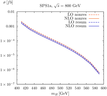
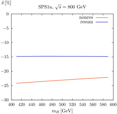
Figure 3: Total cross section $\sigma(e^{+}e^{-}\rightarrow t\bar{b}H^{-})$ (left panel) and relative corrections $\delta$ in percent (right panel) depending on the charged-Higgs-boson mass $m_{H^{\pm}}$ for a center-of-mass energy of $\sqrt{s}=800$ GeV. The other MSSM parameters are taken to have their SPS1a values. Both the nonresummed and resummed cross sections are considered.

  

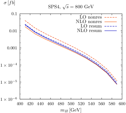
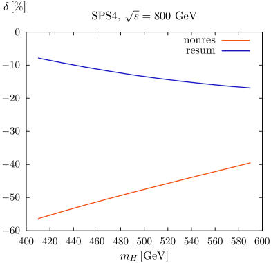
Figure 4: Total cross section $\sigma(e^{+}e^{-}\rightarrow t\bar{b}H^{-})$ (left panel) and relative corrections $\delta$ in percent (right panel) depending on the charged Higgs-boson mass $m_{H^{\pm}}$ for a center-of-mass energy of $\sqrt{s}=800$ GeV. The other MSSM parameters are taken to have their SPS4 values. Both the nonresummed and resummed cross sections are considered.

In Fig. 3, the total cross section $\sigma(e^{+}e^{-}\rightarrow t\bar{b}H^{-})$ is shown for the SPS1a scenario as a function of $m_{H^{\pm}}$ in the range $\sqrt{s}/2<m_{H^{\pm}}<\sqrt{s}-m_{b}-m_{t}$. The cross section falls rapidly with increasing distance from the pair-production threshold at $m_{H^{\pm}}=\sqrt{s}/2=400\,\mathrm{GeV}$. Before resummation, the SUSY-QCD corrections range from $-22\%$ to $-24\%$ and exhibit only a weak dependence on $m_{H^{\pm}}$. After resummation, the residual corrections still amount to about $-15\%$, which implies that the $\tan\beta$-enhanced contributions are not actually dominant for these values of parameters.

Figure 4 shows the $m_{H^{\pm}}$ dependence for the SPS4 scenario with $\tan\beta=50$. In this case, the SUSY-QCD corrections are much larger, ranging from $-40\%$ to $-55\%$. However, the bulk of these corrections is absorbed by the resummation. The size of the residual corrections ranges from $-8\%$ to $-17\%$ and is, therefore, similar to the SPS1a scenario.

  

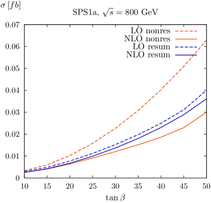
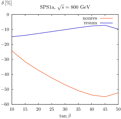
Figure 5: Total cross section $\sigma(e^{+}e^{-}\rightarrow t\bar{b}H^{-})$ (left panel) and relative corrections $\delta$ in percent (right panel) as a function of $\tan\beta$ for a center-of-mass energy of $\sqrt{s}=800$ GeV. The other MSSM parameters have their SPS1a values. Both the nonresummed and resummed cross sections are considered.

In Fig. 5, the $\tan\beta$ dependence of the total cross section $\sigma(e^{+}e^{-}\rightarrow t\bar{b}H^{-})$ is shown for the SPS1a scenario. The cross section grows strongly with increasing value of $\tan\beta$. Without resummation, the relative corrections also show a strong $\tan\beta$ dependence and range from $-24\%$ at low value of $\tan\beta$ up to $-55\%$ at high value of $\tan\beta$. Most of these corrections are absorbed by resummation; the remaining corrections range from $-10\%$ to $-15\%$ and show only a relatively weak dependence on $\tan\beta$. Since we change $\tan\beta$ by modifying the high-energy input parameters, we also need to change $m_{0}$ accordingly to keep the low-energy value of $m_{H^{\pm}}$ at its desired value. This leads to somewhat higher squark masses at high values of $\tan\beta$, so that the loop corrections are suppressed there. Numerically, we find that the competing effects of the loop suppression due to heavier squark masses and of the increase in the bottom Yukawa coupling lead to a maximum in the relative corrections at $\tan\beta\approx 45$. The difference between the nonresummed and resummed NLO cross sections measures the size of the higher-order contributions included by performing the resummation. For high values of $\tan\beta$, these contributions are of similar size to the residual SUSY-QCD corrections underlining the need for resummation in this region.

We note that the analogous analysis of the SUSY-QCD corrections to the associated production of a neutral Higgs boson with a $b\bar{b}$ pair in $e^{+}e^{-}$ annihilation with and without resummation of $\tan\beta$-enhanced contributions yielded similar results [51].

3.1 Comparison of numerical vs analytical loop integral evaluation

$m_{H^{-}}$ [$\,\mathrm{GeV}$] $\sigma_{\text{virt}}^{\text{BT}}\;[\,\mathrm{fb}]$ $\sigma_{\text{virt}}^{\text{ana}}\;[\,\mathrm{fb}]$ 410 -5. 154(7)$\cdot 10^{-4}$ -5. 148(4)$\cdot 10^{-4}$ 450 -8. 46(1)$\cdot 10^{-5}$ -8. 462(6)$\cdot 10^{-5}$ 490 -2. 245(3)$\cdot 10^{-5}$ -2. 245(2)$\cdot 10^{-5}$ 510 -1. 129(2)$\cdot 10^{-5}$ -1. 1295(8)$\cdot 10^{-5}$ 550 -2. 152(3)$\cdot 10^{-6}$ -2. 151(1)$\cdot 10^{-6}$ 590 -1. 409(2)$\cdot 10^{-7}$ -1. 4094(9)$\cdot 10^{-7}$

Table 2: Contribution of the virtual corrections to the total cross section of the process $e^{+}e^{-}\rightarrow t\bar{b}H^{-}$ for a center-of-mass energy of $\sqrt{s}=800\,\mathrm{GeV}$ using the BT and the analytical approaches. The SUSY parameters are chosen according to the SPS1a scenario.

Let us now compare the BT method with the conventional analytical evaluation of the loop integrals. In Table 2, we compare the results for the virtual cross section from Fig. 3 evaluated using the BT method and the analytical loop integrals. The remaining parameters are again chosen according to the SPS1a scenario. Both methods use the same number of points in the numerical integration performed by Vegas, although the dimension of the integral is higher for the numerical approach due to the additional Feynman-parameter integrations. The runtimes of both approaches are also similar. A comparison of the results shows that the agreement between both methods is good, while the errors are typically a factor 1.5 to 3 larger for the BT method. Detailed comparison of the results from Figs. 4 and 5 shows a similar behavior.

  

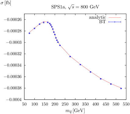
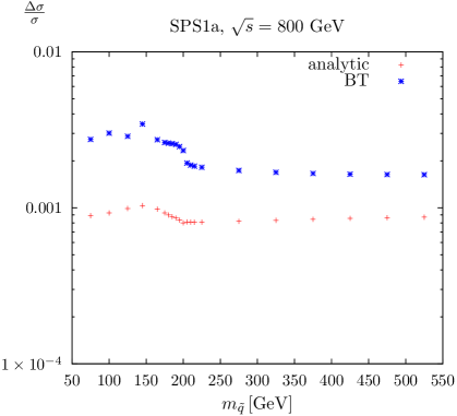
Figure 6: Contribution $\sigma_{\text{virt}}(e^{+}e^{-}\rightarrow t\bar{b}H^{-})$ of the virtual corrections (left panel) to the total cross section and the integration error normalized to the virtual cross section (right panel) as functions of the common squark mass $m_{\tilde{q}}$ for a center-of-mass energy of $\sqrt{s}=800\,\mathrm{GeV}$ using the BT and the analytical methods. The remaining SUSY parameters are chosen according to the SPS1a scenario.

Evaluating single loop integrals using the BT method, we observe that the errors and the runtime may depend sensitively on the presence of thresholds of the particles in the loops. Below all thresholds, the integrand is positive definite in Feynman-parameter space, so that the loop integral is real and the numerical integration is very fast. Once a threshold is crossed, the integrand becomes indefinite, the integrals develop imaginary parts, and the deterministic integration routine needs many more integrand evaluations to reach a reasonable accuracy. In order to find out if this behavior carries over to the combined phase-space and Feynman-parameter integration, we calculate the virtual corrections keeping the center-of-mass energy fixed while varying the squark masses. In this way, we can study the behavior in the vicinity of the various squark-squark thresholds in the loop diagrams. Figure 6 shows the cross section and the integration error for the virtual corrections as a function of a common third-generation squark mass $m_{\tilde{q}}=m_{\tilde{t}_{1}}=m_{\tilde{t}_{2}}=m_{\tilde{b}_{1}}=m_{\tilde{b}_{2}}$. For the remaining parameters, we again use the SPS1a values. If a common squark mass is used, the highest threshold in the loop diagrams is the squark-squark threshold at $m_{\tilde{q}}=\sqrt{s}/2=400\,\mathrm{GeV}$ originating from diagrams of the type shown in Fig. 2(a) and (e). Cutting both squark lines in diagrams (b) or (c), gives another squark-squark threshold at $m_{\tilde{q}}=m_{H^{\pm}}/2\simeq 200\,\mathrm{GeV}$. The squark-squark threshold from diagram (d) is at $m_{\tilde{q}}=s_{tb}/2$, which is constrained by kinematics as $\sqrt{s_{tb}}<\sqrt{s}-m_{H^{\pm}}\simeq 400\,\mathrm{GeV}$. Here, $s_{tb}$ denotes the invariant mass square of the top-bottom system. Since this is close to $m_{H^{\pm}}$ for our choice of parameters, the virtual charged Higgs boson can become almost on-shell resulting in an enhancement of diagram (d). The corresponding threshold below $m_{\tilde{q}}\simeq 200\,\mathrm{GeV}$ may appear to be dominating the behavior of the total cross section in Fig. 6.

The error in the BT method shows a similar qualitative behavior to the error in the analytical method, although it is a factor of 2 to 3 larger. In particular, no increase of the error below the threshold at $m_{\tilde{q}}=400\,\mathrm{GeV}$ can be seen, and the increase in the error below $200\,\mathrm{GeV}$ is only moderate. The strong variation of the errors across thresholds observed when calculating single one-loop integrals in the BT method using a deterministic integration routine is almost completely absent when using the combined phase-space and Feynman-parameter integration.

4 Conclusion

The discovery of charged Higgs bosons would be direct evidence of physics beyond the SM. Since charged Higgs bosons are essential ingredients of all SUSY models and, moreover, future colliders have the potential to detect them, it is worthwhile to study their phenomenology. If the center-of-mass energy of the collider is not sufficient to produce charged-Higgs-boson pairs, the process $e^{+}e^{-}\rightarrow t\bar{b}H^{-}+\text{c.c.}$ is of particular interest. We calculated the cross section of this process in the MSSM to NLO with regard to the strong interaction, by complementing the known SM-QCD corrections [11] by the SUSY-QCD ones.

As for the loop integrations, we deviated from the familiar analytical approach, in which these loop-integrals are expressed in terms of logarithms and dilogarithms. Instead, we adopted the numerical approach of Ref. [25] based on the BT theorem [26] and demonstrated its feasibility for a multileg one-loop calculation such as ours. We compared this alternative method to the conventional analytical approach and found agreement within the numerical errors. In contrast to previous applications of the BT method [31, 32, 33, 34], we were tackling here for the first time a nontrivial phase-space integration and demonstrated how it can be performed simultaneously with the BT integrations.

Concerning the size of the corrections, we found significant SUSY-QCD corrections ranging from $-10\%$ to $-60\%$, which are of similar magnitude to the purely gluonic QCD corrections [11]. The bulk of SUSY-QCD corrections stem from $\tan\beta$-enhanced contributions and can be absorbed by performing a resummation of the bottom-quark Yukawa coupling. The residual corrections after resummation are still sizeable, ranging from $-10\%$ to $-15\%$.

References

- [1] D. P. Roy, Mod. Phys. Lett. A 19, 1813 (2004) [hep-ph/0406102].
- [2] A. Djouadi, J. Kalinowski, and P. M. Zerwas, Z. Phys. C 57, 569 (1993).
- [3] S. Kanemura, S. Moretti, and K. Odagiri, JHEP 0102, 011 (2001) [hep-ph/0012030].
- [4] S.-H. Zhu, Phys. Rev. D 67, 075006 (2003) [hep-ph/0112109].
- [5] G. P. Gao, G. R. Lu, Z. H. Xiong, and J. M. Yang, Phys. Rev. D 66, 015007 (2002) [hep-ph/0202016].
- [6] T. Plehn, Phys. Rev. D 67, 014018 (2003) [hep-ph/0206121].
- [7] E. L. Berger, T. Han, J. Jiang, and T. Plehn, Phys. Rev. D 71, 115012 (2005) [hep-ph/0312286].
- [8] N. Kidonakis, PoS HEP2005, 336 (2006) [hep-ph/0511235].
- [9] S. Komamiya, Phys. Rev. D 38, 2158 (1988).
- [10] J. Guasch, W. Hollik, and A. Kraft, Nucl. Phys. B596, 66 (2001).
- [11] B. A. Kniehl, F. Madricardo, and M. Steinhauser, Phys. Rev. D 66, 054016 (2002) [hep-ph/0205312].
- [12] P. Fayet and S. Ferrara, Phys. Rept. 32, 249 (1977).
- [13] H. P. Nilles, Phys. Rept. 110, 1 (1984).
- [14] H. E. Haber and G. L. Kane, Phys. Rept. 117, 75 (1985).
- [15] G. ’t Hooft and M. Veltman, Nucl. Phys. B153, 365 (1979).
- [16] G. Passarino and M. Veltman, Nucl. Phys. B160, 151 (1979).
- [17] G. J. van Oldenborgh and J. A. M. Vermaseren, Z. Phys. C 46, 425 (1990).
- [18] A. Denner and S. Dittmaier, Nucl. Phys. B734, 62 (2006) [hep-ph/0509141].
- [19] T. Binoth, J.-Ph. Guillet, G. Heinrich, E. Pilon, and C. Schubert, JHEP 0510, 015 (2005) [hep-ph/0504267].
- [20] J. Fleischer and T. Riemann, PoS (ACAT2010), 074 [arXiv:1006.0679].
- [21] T. Diakonidis, J. Fleischer, J. Gluza, K. Kajda, T. Riemann, and J. B. Tausk, Phys. Rev. D 80, 036003 (2009) [arXiv:0812.2134].
- [22] C. F. Berger and D. Forde, Ann. Rev. Nucl. Part. Sci. 60, 181 (2010) [arXiv:0912.3534].
- [23] Z. Bern, L. J. Dixon, and D. A. Kosower, Annals Phys. 322, 1587 (2007) [arXiv:0704.2798].
- [24] Z. Bern et al., (NLO Multileg Working Group), Report No. SLAC-PUB-13206 [arXiv:0803.0494].
- [25] A. Ferroglia, M. Passera, G. Passarino, and S. Uccirati, Nucl. Phys. B650, 162 (2003) [hep-ph/0209219].
- [26] I. N. Bernstein, Functional Analysis and its Applications 6 (1972) 26; F. V. Tkachov, Nucl. Instrum. Meth. A 389, 309 (1997) [hep-ph/9609429].
- [27] G. Passarino and S. Uccirati, Nucl. Phys. B 629, 97 (2002) [hep-ph/0112004].
- [28] A. Ferroglia, M. Passera, G. Passarino and S. Uccirati, Nucl. Phys. B 680, 199 (2004) [hep-ph/0311186].
- [29] S. Actis, A. Ferroglia, G. Passarino, M. Passera and S. Uccirati, Nucl. Phys. B 703, 3 (2004) [hep-ph/0402132].
- [30] G. Passarino and S. Uccirati, Nucl. Phys. B 747, 113 (2006) [hep-ph/0603121].
- [31] W. Hollik, U. Meier and S. Uccirati, Nucl. Phys. B 731, 213 (2005) [hep-ph/0507158].
- [32] G. Passarino, C. Sturm, S. Uccirati, Phys. Lett. B 655, 298 (2007) [arXiv:0707.1401].
- [33] S. Actis, G. Passarino, C. Sturm, and S. Uccirati, Phys. Lett. B 670, 12 (2008) [arXiv:0809.1301].
- [34] S. Actis, G. Passarino, C. Sturm, and S. Uccirati, Nucl. Phys. B811, 182 (2009) [arXiv:0809.3667].
- [35] J. Küblbeck, M. Bohm, A. Denner, Comput. Phys. Commun. 60, 165 (1990); T. Hahn, Comput. Phys. Commun. 140, 418 (2001) [hep-ph/0012260].
- [36] T. Hahn and M. Perez-Victoria, Comput. Phys. Commun. 118, 153 (1999) [hep-ph/9807565].
- [37] G. P. Lepage, J. Comput. Phys. 27, 192 (1978).
- [38] E. Braaten and J. P. Leveille, Phys. Rev. D 22, 715 (1980).
- [39] M. Drees and K. I. Hikasa, Phys. Lett. B 240, 455 (1990); 262, 497(E) (1991); B. A. Kniehl, Nucl. Phys. B376, 3 (1992).
- [40] M. Carena, D. Garcia, U. Nierste, and C. E. M. Wagner, Nucl. Phys. B577, 88 (2000) [hep-ph/9912516].
- [41] J. Guasch, P. Hafliger, and M. Spira, Phys. Rev. D 68, 115001 (2003) [hep-ph/0305101].
- [42] S. Uccirati, Acta Phys. Polon. B 35, 2573 (2004) [hep-ph/0410332].
- [43] M. M. Weber, Acta Phys. Polon. B 35, 2655 (2004) [hep-ph/0410166].
- [44] D. Noth and M. Spira, Phys. Rev. Lett. 101, 181801 (2008) [arXiv:0808.0087].
- [45] D. Noth and M. Spira, arXiv:1001.1935.
- [46] L. Mihaila, C. Reisser, JHEP 1008, 021 (2010) [arXiv:1007.0693].
- [47] B. C. Allanach et al., in Proc. of the APS/DPF/DPB Summer Study on the Future of Particle Physics (Snowmass 2001), edited by N. Graf, Eur. Phys. J. C 25, 113 (2002), eConf C010630 (2001) P125 [hep-ph/0202233].
- [48] N. Ghodbane and H.-U. Martyn, in Proc. of the APS/DPF/DPB Summer Study on the Future of Particle Physics (Snowmass 2001), edited by N. Graf [hep-ph/0201233].
- [49] B. C. Allanach, Comput. Phys. Commun. 143, 305 (2002) [hep-ph/0104145].
- [50] P. Marquard, L. Mihaila, J. H. Piclum and M. Steinhauser, Nucl. Phys. B 773, 1 (2007) [hep-ph/0702185].
- [51] P. Hafliger and M. Spira, Nucl. Phys. B719, 35 (2005) [hep-ph/0501164].