Quasi-Resonant Theory of Tidal Interactions

Abstract

When a spinning system experiences a transient gravitational encounter with an external perturber, a quasi-resonance occurs if the spin frequency of the victim matches the peak orbital frequency of the perturber. Such encounters are responsible for the formation of long tails and bridges of stars during galaxy collisions. For high-speed encounters, the resulting velocity perturbations can be described within the impulse approximation. The traditional impulse approximation, however, does not distinguish between prograde and retrograde encounters, and therefore completely misses the resonant response. Here, using perturbation theory, we compute the effects of quasi-resonant phenomena on stars orbiting within a disk. Explicit expressions are derived for the velocity and energy change to the stars induced by tidal forces from an external gravitational perturber passing either on a straight line or parabolic orbit. Comparisons with numerical restricted three-body calculations illustrate the applicability of our analysis.

1. Introduction

Astrophysical objects dominated by disks supported against gravity by rotation are ubiquitous. They range from planetary rings, to planetary systems, to protoplanetary disks, to accretion disks around young stars and compact objects, to spiral galaxies. Given that astrophysical disks are common, it is not surprising that gravitational encounters involving them and other objects occur frequently. In particular, the numerous examples of peculiar galaxies (e.g., Arp, 1966; Dyson, 1987) suggest that tidal interactions between spirals are a key driver of the morphological transformations of galaxies.

Beginning in the 1960s, various studies established that many peculiar galaxies are, in fact, disks in collision (Pfleiderer & Siedentopf, 1961; Yabushita, 1971; Clutton-Brock, 1972a, b; Wright, 1972; Eneev et al., 1973). However, it was Toomre & Toomre (1972) (hereafter, TT72) who performed the first systematic study of this process, using a restricted three-body technique. In their approach, each galaxy was modeled as a point-particle, representing the potential well, surrounded by a disk of non-interacting test particles (stars) on circular orbits. When two such model galaxies pass by one another, their mutual gravitational tidal forcing distorts the disks as traced by the orbital motion of the test particles in the combined potential of the two point-particles. In this manner, TT72 showed that, contrary to prevailing wisdom, the narrow bridges and tails seen in many peculiar galaxies could be produced by gravity alone, and argued that these features are essentially kinematic in nature.

TT72’s analysis further demonstrated that the bridges connecting pairs of colliding galaxies and the tidal tails that develop continue to lengthen and thin out after an encounter. The well-known systems NGC 4038 (the “Antennae”), NGC 4676 (the “Mice”), and NGC 7252 (the “Atoms for Peace Galaxy”) all have tails extending 50-100 kpc in length (Hibbard & Mihos, 1995). The Superantennae (IRAS19254-7245) is an extreme case in which the tails span 350 kpc from tip to tip (Mirabel et al., 1991). If the galaxies merge, some tail stars may escape the system entirely, but most eventually fall back into the merger remnant, resulting in the formation of “shells” and other fine structures associated with elliptical galaxies (Malin & Carter, 1980) through “phase-wrapping” (Quinn, 1984; Hernquist & Quinn, 1987; Hernquist & Spergel, 1992).

TT72 also showed that the efficiency of “tail-making” depends sensitively on the inclinations of the disks relative to the orbit plane. This is illustrated in Figure 1, which shows the outcome of two of TT72’s simulations in which disks are perturbed by the passage of equal-mass companions on parabolic orbits. The collisions are co-planar, meaning that the victim disks lie exactly in the orbit plane, but in the top row of Figure 1 the encounter is prograde, so that the internal spin of the disk is aligned with the direction of the orbital angular momentum, whereas in the bottom row the two are anti-parallel, defining a precisely retrograde interaction.

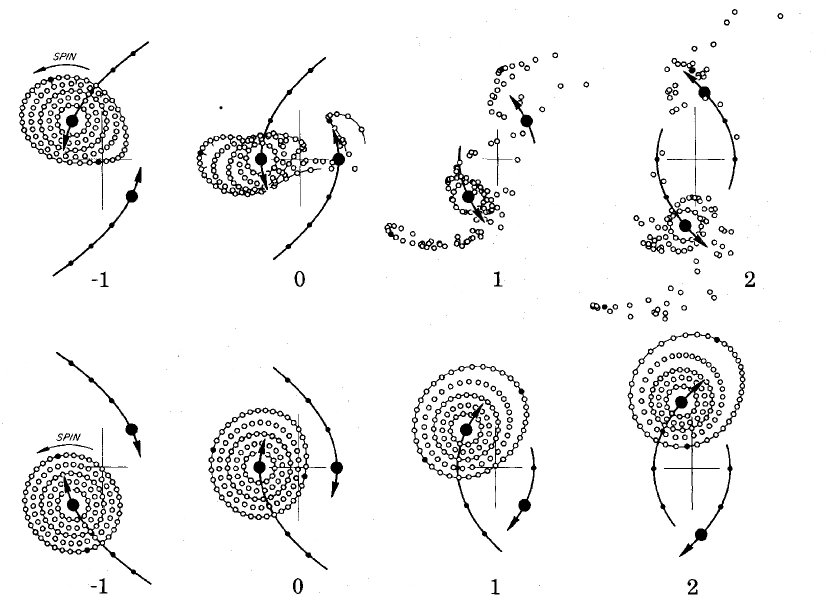
Figure 1.— Tail-making during a prograde encounter between two equal-mass galaxies, represented by point-particles is shown in top row. For clarity, the test particles comprising only one of the disks are plotted. In prograde collisions, the stars in the disk are in near-resonance with the perturber during the interaction and are continuously pulled either inward or outward, depending on their internal orbital phases in relation to the orbital motion of the perturber. A retrograde version of the encounter is shown in the bottom row. In this case, the stars in the disk are pulled alternately inward and outward during the collision, with little net effect. (Adapted from Toomre & Toomre, 1972)

It is obvious from visual inspection of Figure 1 that prograde encounters can do much more violence to spinning disks than retrograde ones. TT72 interpreted this difference physically as owing to a “near-resonance or matching of their [internal] orbital speeds with the peak angular motion of the companion.” In other words, a relatively strong response follows if the spin angular frequency of the disk is aligned with and of similar magnitude to the orbital angular frequency of the collision at pericenter. If the stars in the disk are on circular orbits, but the trajectory of the interaction is non-circular (as in the examples of parabolic orbits shown in Figures 1), then the orbital angular frequency varies with time and the resonance is only temporary; hence, a “near-” or “quasi-resonance.” Mathematically, the condition for a strong response is expressed by

$$\Omega_{\rm{disk}}=\Omega_{\rm{orb}}\ \ \rightarrow\ \ \frac{v}{r}\sim\frac{V}{R\sqrt{(1+e)}},$$ (1)

where $v$ and $r$ are the internal rotation velocity and characteristic size of the disk, respectively, $V$ and $R$ are the orbit velocity and separation at pericenter, and $e$ the eccentricity of the orbit (Binney & Tremaine, 1987).

The work of Barnes (1988, 1992) and Hernquist (1992, 1993) generalized TT72’s modeling by treating the internal gravity of colliding galaxies self-consistently. These and related studies verified TT72’s claim that tail-making is a kinematic process (see Figure 3 of Dubinski et al., 1999) and examined the sensitivity of tail-making efficiency to the distribution of stars in interacting and merging galaxies.

Subsequently, Dubinski et al. (1996) and Mihos et al. (1998) demonstrated empirically that the lengths and kinematics of tidal tails also depend critically on the distribution of dark matter surrounding each galaxy. For the same radial stellar profiles, longer (shorter) and more (less) prominent tidal tails form in shallower (deeper) dark matter potential wells. In particular, Dubinski et al. (1999) and Springel & White (1999) showed that the depth of the dark matter potential is as important in determining the lengths of tidal tails as the orbit (see e.g. Figure 4 in Dubinski et al., 1999). Similar conclusions have been reached in studies of local dwarf spheroidal galaxies (see e.g. Mayer et al., 2002; Read et al., 2006).

Most recently, it has been shown that resonant stripping of stars in disks can alter the mass to light ratios of dwarf galaxies when they encounter more massive systems by removing luminous material more efficiently than dark matter. The minimal response of the dark matter is expected if its particles move on random orbits, in which case the net perturbation on the halo mostly averages out (D’Onghia et al., 2009). A similar resonant phenomenon has been suggested to cause the LMC disk to thicken by interactions with the Milky Way (Weinberg, 2000) or more generally in the context of heating and disruption of satellites (Choi et al., 2009). In addition, the origin of the Magellanic Stream might have a tidal origin (Besla et al., 2010) through interactions between dwarfs in groups (D’Onghia & Lake, 2008), provided that the Magellanic Clouds are on their first pericentric passage (Kallivayalil et al., 2006; Besla et al., 2007).

While these works have elucidated the physics of tail-making and proven that observed peculiar galaxies are indeed a consequence of collisions and mergers, they have left open a number of important issues. Most previous studies of tidal interactions between disk galaxies have been empirical in nature. Thus, they have identified broad conditions for tidal features to be produced, but have not provided simple criteria for isolating the efficiency of this process on specific parameters of an encounter. Therefore, the circumstances under which very long tails could result, like those in the Superantennae, remain uncertain. Moreover, even nearly 40 years after TT72, there is still considerable confusion in the community regarding galactic bridges and tails, especially in regards to the role played by resonances in their origin. Finally, attempts to reproduce the morphology and kinematics of individual observed systems is greatly complicated by the sensitivity of tail-making to the distribution of dark matter around galaxies.

One approach for dealing with this last issue is to survey the vast parameter space that allows for variations in the orbit, the relative masses and spatial sizes of the luminous galaxies, and the dark matter potentials. A promising scheme along these lines has been developed recently by Barnes & Hibbard (2009) with their Identikit algorithm. In what follows, we pursue a complementary technique by formulating a simple analytic description of tail-making to understand it from an alternate perspective. Our methodology necessarily entails various approximations and is hence less general than simulation-based procedures, but makes it possible to identify scalings of, and interpret physically, the response of rotating objects to gravitational tidal perturbations. While our immediate attention is devoted to galactic disks, our formalism is general with respect to the system under consideration, so we anticipate that our analysis will be relevant to a wide range of tidal phenomena.

In §2, we describe our method for analyzing tidal responses of rotating systems. We adopt a variant of the impulse approximation in which we allow particles in the perturbed system to move along their internal, unperturbed orbits during the encounter. In §3, we derive analytic expressions in terms of special functions for the velocity perturbations delivered to spinning disks in these interactions, in the case of coplanar collisions. We do this first for high-speed, straight-line trajectories, in §3.1, and then for parabolic orbits in §3.2, the latter based partly on the work of Press & Teukolsky (1977) for tidal interactions between stars. We present numerical examples and contrast the straight-line and parabolic cases in §3.3. In §4, we generalize our formalism to non-coplanar encounters, for both straight-line and parabolic orbits. We compare the results of our analytic prescriptions to simulations of tidal interactions in §5. Finally, we summarize and conclude in §6.

2. Methodology

Our approach is based on a variant of the impulse approximation for studying gravitational perturbations on systems. In some respects, our formalism has similarities to that of Press & Teukolsky (1977), who considered tidal interactions between stars as a means for forming close binaries. Press & Teukolsky (1977) calculated the response of gas spheres to external gravitational perturbations and the energy deposited into non-radial oscillations. Later, similar analytic estimates of the energy and angular momentum exchange between a circumstellar disk and a passing star on a near-parabolic orbit were inferred by Ostriker (1994) in the context of accretion disks.

Consider a flat, rotationally supported disk of stars, perturbed gravitationally by a passing object. In the usual impulse approximation (Binney & Tremaine, 1987), it is assumed that the stars in the perturbed system remain strictly stationary during the course of the encounter. The tidal force from the perturber relative to the center of mass of the perturbed body is calculated at each location within it from each point along the relative orbit of the interaction. The total velocity impulse delivered to each star in the perturbed object is then calculated by integrating the force over the entire orbit. In the simplest application of this method, the perturber follows a straight-line trajectory, as for a high-speed encounter, although as we show in what follows, it is possible to generalize the technique also to parabolic collisions, following Press & Teukolsky (1977).

The analytic expressions that result from the impulse approximation (Spitzer, 1958) give reasonably accurate results for the energy deposited in objects during tidal encounters for systems that are dominated by internal random motions (Gallagher & Ostriker, 1972; Dekel et al., 1980; Aguilar & White, 1985; D’Onghia et al., 2010). However, this method is not appropriate for capturing the essentials of responses like those in Figures 1 because, by construction, it does not distinguish between prograde and retrograde interactions, since the stars in the perturbed body are held fixed during the encounter.

To qualitatively capture the influence of resonances during tidal interactions, we employ the following variant of the impulse approximation. During the course of the encounter, stars in the perturbed system are allowed to move along unperturbed orbits within their host. For simplicity, we assume that the unperturbed orbits are strictly circular, although modest departures from these paths could, in principle, be handled using epicyclic theory. In this manner, the response of a given star will depend not only on its spatial location within the perturbed system, but also its velocity. As we demonstrate explicitly below, this approach makes it possible to characterize the resonant aspects of tidal interactions that distinguish between prograde and retrograde collisions, as in Figure 1.

If the orbit of the encounter is non-circular, as in the examples that follow, the orbital angular frequency varies with time and, so, a given star within the perturbed system will be in precise resonance with the motion of the perturber for only a limited time. For this reason, we will refer to the formalism herein as describing quasi-resonant behavior, meaning that the response only resembles that characteristic of a true resonant interaction. This meaning should be taken to be equivalent to TT72’s description of tidal interactions between spinning objects as displaying “near-resonant” qualities.

To be specific, consider a disk of stars on circular orbits comprising the victim interacting with an object which we will refer to as the perturber. Employ a coordinate system with origin at the center of mass of the victim and assume that the disk is razor thin and orient the coordinate system so that the disk is in the $x-y$ plane. Then, the coordinate vector to any star within the victim is given by

$$\overrightarrow{r}(t)=(x(t),y(t),0)=(r\cos\phi(t),r\sin\phi(t),0),$$ (2)

where $r$ is constant, because we assume that the unperturbed orbits internal to the victim are circular, and the position vector to the perturber will be denoted by

$$\overrightarrow{R}(t)=(X(t),Y(t),Z(t))\,.$$ (3)

In the sections below, we will consider various choices for the trajectory $\overrightarrow{R}(t)$, which will fix the time-dependence of the components $(X(t),Y(t),Z(t))$. We will adopt the convention that the unperturbed disk always lies in the $x-y$ plane. Thus, for non-coplanar encounters, we will incline the orbit plane defined by the trajectory $\overrightarrow{R}(t)$ so that $Z(t)$ will be non-zero.

The acceleration of each star relative to that on the center of mass of the perturbed body is

$${{d\overrightarrow{v}}\over{dt}}=-\left[\nabla\Psi\,-\,{1\over M}\int\rho(\overrightarrow{r}^{\prime})\nabla\Psi(\overrightarrow{r}^{\prime})d^{3}\overrightarrow{r}^{\prime}\right]\,,$$ (4)

where $\Psi$ is the interaction potential between the perturber and the victim, $M$ is the mass of the victim, and the integral is over the density profile of this object. Expand $\nabla\Psi$ about the origin in a Taylor series using

$$\Xi(\overrightarrow{r}+\overrightarrow{a})\,=\,\sum_{n=0}^{\infty}\,{1\over{n!}}\left(\overrightarrow{a}\cdot\nabla\right)^{n}\,\Xi(\overrightarrow{r})\,.$$ (5)

After algebra, taking into account that the origin is located at the center of mass of the victim, the $k$-th component of the acceleration becomes

$${{dv_{k}}\over{dt}}=-\Biggl{\{}\sum_{j}r_{j}\left({{\partial^{2}\Psi}\over{\partial r_{j}\partial r_{k}}}\right)_{\overrightarrow{r}=0}\,+\,{1\over 2}\sum_{l}\sum_{j}\left[\left(r_{j}r_{l}\,-\,H_{jl}\right)\,\left({{\partial^{3}\Psi}\over{\partial r_{l}\partial r_{j}\partial r_{k}}}\right)_{\overrightarrow{r}=0}\right]\,+\,\ldots\,\Biggr{\}}\,,$$ (6)

where $H_{jl}\equiv I_{jl}/M$ and $I_{jl}$ is the moment of inertia tensor (Binney & Tremaine, 1987):

$$I_{jl}\,\equiv\,\int\rho r_{j}r_{l}d^{3}\overrightarrow{r}\,.$$ (7)

For simplicity, treat the force on each star in the disk from the perturber as that from a point mass. Then, the interaction potential is

$$\Psi=-{{GM_{\rm pert}}\over{\left|\overrightarrow{r}(t)-\overrightarrow{R}(t)\right|}}.$$ (8)

Performing the derivatives required in the above expression, we obtain the acceleration of a particular star at a given time. The velocity impulse delivered by the encounter can then be obtained by integrating over time. Thus, the leading term in the series is (Binney & Tremaine, 1987)

$$\Delta\overrightarrow{v}\,=\,-GM_{\rm pert}\,\int_{-\infty}^{\infty}\left[{\overrightarrow{r}\over{R^{3}}}\,-\,3{{\overrightarrow{R}(\overrightarrow{r}\cdot\overrightarrow{R})}\over{R^{5}}}\right]dt\,.$$ (9)

Likewise, the next order correction term can be written

$$\Delta\overrightarrow{v}_{corr}\,=\,-{3\over 2}GM_{\rm pert}\,\int_{-\infty}^{\infty}{1\over{R^{5}}}\Biggl{\{}2\overrightarrow{r}(\overrightarrow{r}\cdot\overrightarrow{R})\,+\,\left(r^{2}-Tr({\bf H})-2{\bf H}\right)\overrightarrow{R}\,+\,5{{\overrightarrow{R}}\over{R^{2}}}\left[(\overrightarrow{R}\cdot{\bf H}\overrightarrow{R})-(\overrightarrow{r}\cdot\overrightarrow{R})^{2}\right]\Biggr{\}}dt\,.$$ (10)

In principle, this procedure can be extended to even higher order terms in the series. Note that the terms in this last equation are all $\sim O(r^{2})$ since the elements in the matrix ${\bf H}$ involve integrals over squares of the internal coordinates of the victim, while the terms in eq. (9) are $\sim O(r)$.

In what follows, we will employ eq. (9) as the starting point for our analysis. Unlike as in the usual impulse approximation we will allow both $\overrightarrow{R}(t)$ and $\overrightarrow{r}(t)$ to vary in time. We will, however, assume that the trajectory of the interaction, specified by $\overrightarrow{R}(t)$, is prescribed (i.e. orbital decay is not accounted for), and that the orbital motion within the victim, set by $\overrightarrow{r}(t)$, is such that the stars follow their unperturbed motions throughout the course of the interaction.

3. Coplanar Encounters

To illustrate our approach, we begin by considering a coplanar interaction between a perfectly thin, rotating disk of stars and a passing perturber. As noted earlier, the origin of the coordinate system will be at the center of mass of the victim and the coordinate system will be oriented so that the disk lies in the $x-y$ plane. While not general, this case suffices to characterize the dynamics of such encounters; we will generalize to non-coplanar collisions later. Denote the mass of the victim disk by $M$ and that of the perturber by $M_{\rm{pert}}$.

3.1. Straight-line trajectory

The case of a perturber moving along a straight line relative to the victim is the simplest one to analyze and is appropriate for high-speed encounters, as in clusters of galaxies. For definiteness, take the orbit path to be

$$\overrightarrow{R}(t)=(b,V_{sl}\,t,0)\,,$$ (11)

where, as indicated in Figure 2, $b$ is the distance of closest approach (the impact parameter), which occurs at time $t=0$, and $V_{sl}$ is the velocity of the encounter, which is constant for a straight-line trajectory. The internal motions of the disk particles are given by eq. (2) with

$$\phi(t)=\Omega t+\phi_{0}\,,$$ (12)

where $\Omega$ the internal angular frequency of the victim and $\phi_{0}$ is the phase at the minimum distance from the perturber at $t=0$. Note that while $\Omega$ is assumed to be constant in time, it can vary spatially according to $\Omega=\Omega(r)$, depending on the shape of the rotation curve of the victim. We will adopt the convention that $b$ and $V_{sl}$ are non-negative and distinguish prograde versus retrograde collisions for co-planar encounters by the sign of $\Omega=\pm\mid\Omega\mid$ so that

$$\Omega>0\ \ \ \ \ \ \ \ \ \rm{for}\ \rm{prograde}\ \rm{coplanar}\ \rm{encounters}\ \ \ \ \ \ \ \ \ \ \ \ \ \ \$$

$$\ \Omega<0\ \ \ \ \ \ \ \ \ \rm{for}\ \rm{retrograde}\ \rm{coplanar}\ \rm{encounters}\,.\ \ \ \ \ \ \ \ \ \ \ \$$

We further define the non-negative parameter $\alpha$ by

$$\alpha=\frac{\mid\Omega\mid b}{V_{sl}}\,.$$ (14)

The orbital angular frequency varies with time along the trajectory according to

$$\Omega_{orb}(R)\,=\,{{V_{sl}}\over R}={{V_{sl}}\over{b(1+u^{2})^{1/2}}}\,,$$ (15)

where $u=V_{sl}\,t/b$. At the distance of closest approach, when $t=0$, $\Omega_{orb}(b)=V_{sl}/b$ and so physically

$$\alpha={{\mid\Omega\mid}\over{\Omega_{orb}(b)}}$$ (16)

describes the condition for a resonance, with a strong response expected for $\alpha\sim 1$ when $\Omega>0$.

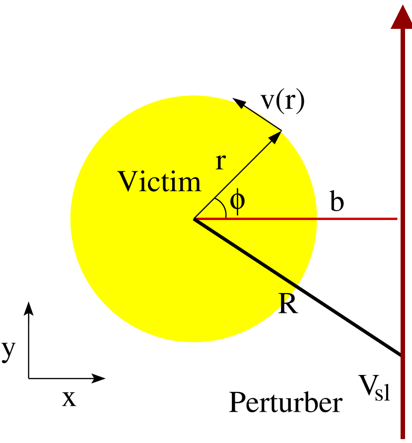
Figure 2.— Schematic view of a spinning disk galaxy (the victim) encountering a perturber passing by on a straight line at a constant speed $V_{sl}$. The stars in the victim are assumed to move on circular orbits.

Employing the usual trigonometric relations

$$\rm{cos}(\Omega t+\phi_{0})=\rm{cos}\Omega t\cdot\rm{cos}\phi_{0}-\rm{sin}\Omega t\cdot\rm{sin}\phi_{0}$$ (17)

$$\rm{sin}(\Omega t+\phi_{0})=\rm{sin}\Omega t\cdot\rm{cos}\phi_{0}+\rm{cos}\Omega t\cdot\rm{sin}\phi_{0}$$ (18)

and substituting into eq. (9) gives

$$\Delta\rm{v}_{x}=-\rm{GM}_{\rm{pert}}\frac{\rm{r\ cos}\phi_{0}}{\rm{b}^{2}\rm{V_{sl}}}\int_{-\infty}^{\infty}\Big{[}\frac{\rm{cos}(\alpha\rm{u})}{(1+\rm{u}^{2})^{3/2}}-3\frac{\rm{cos}(\alpha\rm{u})}{(1+\rm{u}^{2})^{5/2}}\mp 3\rm{u}\frac{\rm{sin}(\alpha\rm{u})}{(1+\rm{u}^{2})^{5/2}}\Big{]}\rm{du}$$ (19)

$$\Delta\rm{v}_{y}=-\rm{GM}_{\rm{pert}}\frac{\rm{r}\sin\phi_{0}}{\rm{b}^{2}\rm{V_{sl}}}\int_{-\infty}^{\infty}\Big{[}-\frac{2\rm{cos}(\alpha\rm{u})}{(1+\rm{u}^{2})^{3/2}}\pm 3\rm{u}\frac{\rm{sin}(\alpha\rm{u})}{(1+\rm{u}^{2})^{5/2}}+3\frac{\cos(\alpha\rm{u})}{(1+\rm{u}^{2})^{5/2}}\Big{]}\rm{du}$$ (20)

and $\Delta v_{z}=0$. In these expressions, for the terms with $\mp$ or $\pm$ symbols the upper and lower signs correspond to prograde and retrograde cases, respectively.

These integrals can be evaluated in terms of the modified Bessel functions $K_{1}$ and $K_{2}$ (Abramowitz & Stegun, 1972). Employing the recursion relation

$$\alpha K_{2}(\alpha)=\alpha K_{0}(\alpha)+2K_{1}(\alpha)$$ (21)

we arrive at

$$\Delta\rm{v}_{x}=2\rm{GM}_{\rm{pert}}\frac{\rm{r\ cos}\phi_{0}}{\rm{b}^{2}\rm{V_{sl}}}\Big{[}\alpha K_{1}(\alpha)+\alpha^{2}\Big{(}K_{0}(\alpha)\pm K_{1}(\alpha)\Big{)}\Big{]}$$ (22)

$$\Delta\rm{v}_{y}=-2\rm{GM}_{\rm{pert}}\frac{\rm{r\ sin}\phi_{0}}{\rm{b}^{2}\rm{V_{sl}}}\Big{[}\alpha^{2}\Big{(}K_{0}(\alpha)\pm K_{1}(\alpha)\Big{)}\Big{]},$$ (23)

where the upper and lower signs are for prograde and retrograde encounters, respectively, and $\Delta$v_z=0 for coplanar collisions. The structure of the expressions in terms of the modified Bessel functions $K_{0}$ and $K_{1}$ is reminiscent of the results describing the perturbations of orbits of stars within disks owing to passing molecular clouds (Julian & Toomre, 1966).

It is of interest to consider various limiting cases for these expressions. When $\alpha\rightarrow 0$, corresponding to a slowly rotating system, the Bessel functions asymptote to $K_{0}(\alpha)\sim-\ln\alpha$ and $K_{1}(\alpha)\sim 1/\alpha\$ (Abramowitz & Stegun, 1972), and we find

$$\Delta\rm{v}_{x}\rightarrow 2\frac{\rm{GM}_{\rm{pert}}}{\rm{b}^{2}\rm{V_{sl}}}\rm{r\ cos}\phi_{0}\ \ \ \ \ \ \ \rm{for}\ \alpha\rightarrow 0$$ (24)

$$\Delta\rm{v}_{y}\rightarrow 0\ \ \ \ \ \ \ \ \ \ \ \ \ \ \ \ \ \ \ \ \ \ \ \ \ \ \ \ \ \ \ \ \ \rm{for}\ \alpha\rightarrow 0$$ (25)

which can be obtained from the usual result for the impulse approximation (eq. (7-54) in Binney & Tremaine, 1987), as this limit describes the situation when the stars in the disk remain nearly stationary during the collision. Note that this limit is insensitive to the sign of $\Omega$ and hence does not distinguish between prograde and retrograde encounters.

The limit $\alpha\rightarrow\infty$ corresponds to an interaction where the response should be weak because, for example, the encounter is a distant one or the spin and orbital frequencies are highly mismatched. Employing the asymptotic expansion for the Bessel functions (Abramowitz & Stegun, 1972),

$$K_{\nu}(\alpha)\sim\frac{\sqrt{\pi}e^{-\alpha}}{\sqrt{2\alpha}}\Big{[}1+\frac{\mu-1}{8\alpha}+\frac{(\mu-1)(\mu-9)}{2!(8\alpha)^{2}}+...\Big{]}\,,$$ (26)

where $\mu=4\nu^{2}$, we find for the prograde and retrograde cases separately:

$$(\Delta\rm{v}_{x})_{\rm{pro}}\sim 2\frac{\rm{G}\rm{M}_{\rm{pert}}}{\rm{b}^{2}\rm{V_{sl}}}r\cos\phi_{0}\Big{(}\sqrt{2\pi}\alpha^{3/2}e^{-\alpha}\Big{)}$$ (27)

$$(\Delta\rm{v}_{y})_{\rm{pro}}\sim-2\frac{\rm{GM}_{\rm{pert}}}{\rm{b}^{2}\rm{V_{sl}}}r\sin\phi_{0}\Big{(}\sqrt{2\pi}\alpha^{3/2}e^{-\alpha}\Big{)}$$ (28)

$$(\Delta\rm{v}_{x})_{\rm{retro}}\sim 2\frac{\rm{GM}_{\rm{pert}}}{\rm{b}^{2}\rm{V_{sl}}}r\cos\phi_{0}\Big{(}\frac{\sqrt{\pi}}{2^{3/2}}\alpha^{1/2}e^{-\alpha}\Big{)}$$ (29)

$$(\Delta\rm{v}_{y})_{\rm{retro}}\sim 2\frac{\rm{GM}_{\rm{pert}}}{\rm{b}^{2}\rm{V_{sl}}}r\sin\phi_{0}\Big{(}\frac{\sqrt{\pi}}{2^{3/2}}\alpha^{1/2}e^{-\alpha}\Big{)}.$$ (30)

We note that the response is exponentially suppressed in the limit $\alpha\rightarrow\infty$, which demonstrates explicitly that the perturbed system is protected by adiabatic invariance. It is also interesting that in this limit the prograde and retrograde cases are simply related:

$$\frac{(\Delta\rm{v}_{x})_{\rm{pro}}}{(\Delta\rm{v}_{x})_{\rm{retro}}}\sim 4\alpha$$ (31)

and for the y-component:

$$\frac{(\Delta\rm{v}_{y})_{\rm{pro}}}{(\Delta\rm{v}_{y})_{\rm{retro}}}\sim-4\alpha\,.$$ (32)

Thus, the prograde response diverges relative to the retrograde one, by a factor of $\alpha$, and, for a given $\alpha$ the magnitude in the velocity perturbation is exactly a factor of four larger.

From the above expressions, the change in the energy of the perturbed system can be determined from:

$$(\Delta\rm{E})_{sl}=\frac{1}{2}\int\rho(\overrightarrow{r})\mid\Delta\rm{v}\mid^{2}d^{3}\overrightarrow{r}=\frac{2\rm{G}^{2}\rm{M}_{\rm{pert}}^{2}}{\rm{b}^{4}\rm{V_{sl}}^{2}}\int_{0}^{\infty}r^{3}dr\Sigma(r)\cdot\hskip 113.81102pt$$

$$\int_{0}^{2\pi}\Big{[}\Big{(}\alpha^{2}K_{0}(\alpha)+\alpha(1\pm\alpha)K_{1}(\alpha)\Big{)}^{2}\cos^{2}\phi+\alpha^{4}\Big{(}K_{0}(\alpha)\pm K_{1}(\alpha)\Big{)}^{2}\sin^{2}\phi\Big{]}d\phi\,,\ \ \ \ \ \ \ \ \ \ \ \ \$$ (33)

where it is assumed that the disk is axisymmetric and has zero vertical thickness, and $\Sigma(r)$ denotes the surface mass density distribution. Doing the angular integral gives

$$(\Delta\rm{E})_{sl}=\frac{2\rm{G}^{2}\rm{M}_{\rm{pert}}^{2}\pi}{\rm{b}^{4}\rm{V_{sl}}^{2}}\int_{0}^{\infty}\rm{r}^{3}\rm{dr}\Sigma(r)\cdot\hskip 227.62204pt\ \ \ \ \ \ \ \ \ \ \ \ \$$

$$\Big{[}2\alpha^{4}K_{0}^{2}(\alpha)+2\alpha^{3}\Big{(}1\pm 2\alpha\Big{)}K_{0}(\alpha)K_{1}(\alpha)+\alpha^{2}\Big{(}2\alpha^{2}\pm 2\alpha+1\Big{)}K_{1}^{2}(\alpha)\Big{]}\,.\ \ \ \ \ \ \ \ \ \ \ \ \ \ \ \$$ (34)

In the limit $\alpha\rightarrow 0$, the energy change is

$$(\Delta\rm{E})_{sl}\sim 2\pi\frac{\rm{G}^{2}\rm{M}_{\rm{pert}}^{2}}{\rm{b}^{4}\rm{V_{sl}}^{2}}\int_{0}^{\infty}\rm{dr}r^{3}\Sigma(r)\,,$$ (35)

which agrees with the corresponding expression in Binney & Tremaine (1987) using the impulse approximation, as expected, while in the limit $\alpha\rightarrow\infty$ for the prograde case

$$(\Delta\rm{E})_{\rm{pro}}\sim\frac{8\pi^{2}\rm{G}^{2}\rm{M}_{\rm{pert}}^{2}}{\rm{b}^{4}\rm{V_{sl}}^{2}}\int_{0}^{\infty}\rm{dr}r^{3}\Sigma(r)\alpha^{3}e^{-2\alpha}$$ (36)

and for a retrograde encounter

$$(\Delta\rm{E})_{\rm{retro}}\sim\frac{\pi^{2}\rm{G}^{2}\rm{M}_{\rm{pert}}^{2}}{2\rm{b}^{4}\rm{V_{sl}}^{2}}\int_{0}^{\infty}\rm{dr}r^{3}\Sigma(r)\alpha e^{-2\alpha}\,.$$ (37)

To evaluate these, or eq. (34), it is necessary to specify the radial dependence of $\alpha(r)$, i.e., the shape of the rotation curve of the victim.

We have also evaluated the next order correction term given by equation (10), yielding:

$$\Delta v^{corr}_{x}\,=\,-\frac{GM_{\rm pert}r^{2}}{b^{3}V_{sl}}\,\Biggr{\{}-1+\frac{2H}{r^{2}}+{\rm cos}2\phi_{0}\Bigg{[}-2\alpha^{2}\Big{(}1\pm 4\alpha\Big{)}K_{0}(2\alpha)-2\alpha\Big{(}1\pm 2\alpha+4\alpha^{2}\Big{)}K_{1}(2\alpha)\Bigg{]}\Biggr{\}}$$ (38)

$$\Delta v^{corr}_{y}\,=\,-\frac{GM_{\rm pert}r^{2}}{b^{3}V_{sl}}{\rm sin}2\phi_{0}\cdot 2\alpha\,\Biggr{\{}\pm 4\alpha^{2}K_{0}(2\alpha)+K_{1}(2\alpha)\Big{(}4\alpha^{2}\pm\alpha\Big{)}\Biggr{\}},$$ (39)

where the upper and lower signs terms refer to prograde and retrograde encounters, respectively, and $\Delta$v${}_{z}=0$ because the encounter is assumed to be coplanar. We note that the $H$ term does not couple to the phase $\phi_{0}$ of an individual star, because it describes the overall reaction of the victim to the perturber; i.e. the gain of angular momentum of the entire disk. On top of this global contribution, each star also receives a resonant sensitive and $\phi_{0}$ dependent contribution. A similar effect occurs in linear order. There, the overall contribution leads to a motion of the center of mass of the victim. But since our calculation is performed in the center of mass reference frame, this $\phi_{0}$ independent contribution does not show up explicitly in the linear order results. There all terms depend on the phase $\phi_{0}$. We further note that the argument of the trigonometric functions involving $\phi_{0}$ is different in first and second order: $\phi_{0}$ in linear order and $2\phi_{0}$ in second order. This implies, that the coupling of both orders leads to an asymmetric perturbation in $x$ and $y$, whereas the linear term alone always produces symmetric results as can be seen from the velocity increments in the $x$ and $y$ directions.

3.2. Parabolic trajectory

Next, consider an encounter from a parabolic trajectory, which is the case analyzed by Press & Teukolsky (1977) in their study of tidal interactions between stars. This situation is relevant for collisions between galaxies in the field or in loose groups, where the orbits are highly elongated. For this reason, TT72 focused on this geometry in particular, as in the examples shown in Figure 1.

The relative velocity between the victim and perturber in this case is their mutual escape velocity, treating the interaction as that between two point masses, and is given by:

$$\rm{V_{p}}(\rm{R})=\Big{[}\frac{2\rm{G}(\rm{M}_{\rm{pert}}+\rm{M})}{\rm{R}}\Big{]}^{1/2}\,.$$ (40)

At the minimum separation between the victim and the perturber the relative velocity attains its maximum value V₀:

$$\rm{V_{p}}(\rm{b})=\rm{V}_{0}=\Big{[}\frac{2\rm{G}(\rm{M}_{\rm{pert}}+\rm{M})}{\rm{b}}\Big{]}^{1/2}$$ (41)

and the relative velocity can be written as

$$\rm{V_{p}(R)}=V_{0}\Big{(}\frac{b}{R}\Big{)}^{1/2}\,.$$ (42)

We orient the disk as in the earlier derivation, so the orbits within the victim disk are given again by eqs. (2) and (12). To specify the orbit path, employ polar coordinates and write

$$\overrightarrow{R}(t)=(X(t),Y(t),0)=(R(t)\cos\Phi(t),R(t)\sin\Phi(t),0)\,.$$ (43)

The orbit is then specified parametrically by the relations (Press & Teukolsky, 1977)

$$\rm{R}=\rm{b}(1+\xi^{2})$$ (44)

and

$$\xi=\rm{tan}\Big{(}\frac{\Phi}{2}\Big{)},$$ (45)

so that the trajectory can be written as

$$Y^{2}=4b^{2}\Big{(}1-\frac{X}{b}\Big{)}\,.$$ (46)

A schematic illustration of this case is shown in Figure 3.

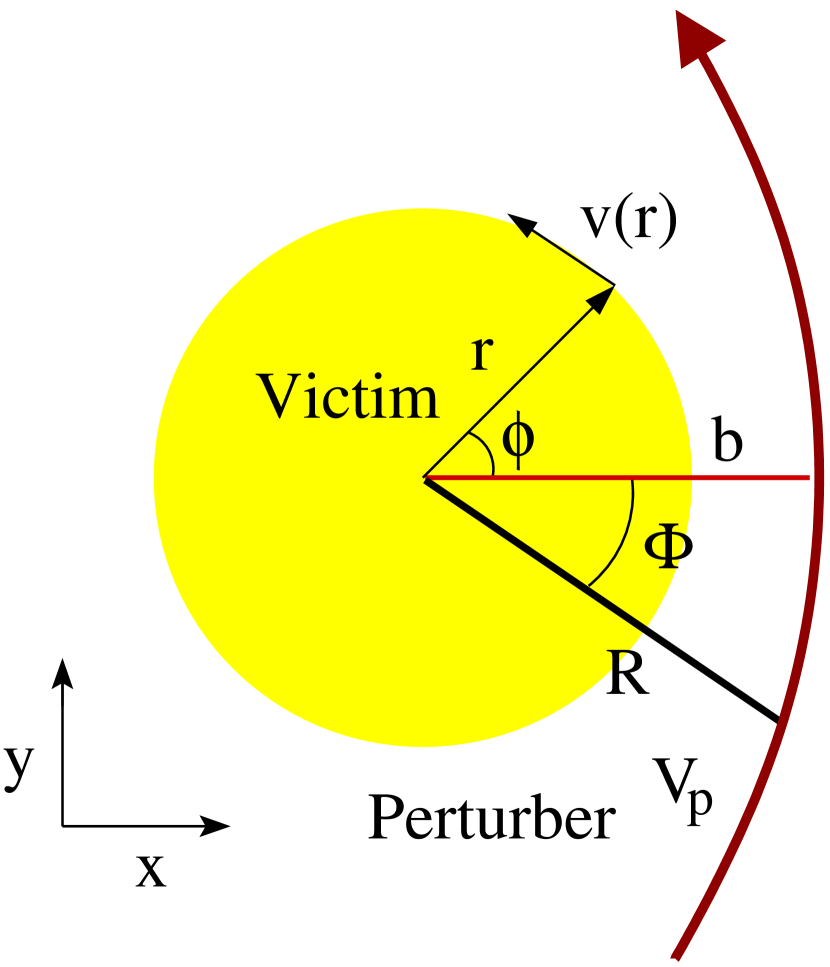
Figure 3.— Schematic view of a spinning disk galaxy (the victim) encountering a perturber on a parabolic orbit.

The time-dependence of the orbit is given implicitly by the relation

$$\rm{t}=\Big{[}\frac{2\rm{b}^{3}}{\rm{G}(\rm{M}+\rm{M}_{\rm{pert}})}\Big{]}^{1/2}(\xi+\frac{1}{3}\xi^{3})=\frac{2\rm{b}}{\rm{V}_{0}}(\xi+\frac{1}{3}\xi^{3})\,.$$ (47)

We again introduce the parameter

$$\alpha=\frac{\mid\Omega\mid b}{V_{0}},$$ (48)

with $\Omega=\pm\mid\Omega\mid$, where the plus and minus signs are for prograde and retrograde coplanar encounters, respectively. The orbital angular frequency is

$$\Omega_{orb}(R)\,=\,{{V_{p}}\over R}={{V_{0}}\over{b}}\left({b\over R}\right)^{3/2}\,,$$ (49)

so that, as in the case of the straight-line trajectory

$$\alpha={{\mid\Omega\mid}\over{\Omega_{orb}(b)}}\,,$$ (50)

and the largest response is expected for $\alpha\sim 1$.

To evaluate the velocity perturbations in this case, we begin with eq. (9) and adopt the time dependence of the motion within the victim from eq. (2). The phase angle of the stellar orbits within the victim is given by

$$\phi(t)=\pm 2\alpha(\xi+\frac{1}{3}\xi^{3})+\phi_{0}\,.$$ (51)

Expand $\cos\phi(t)$ and $\sin\phi(t)$ using trigonometric relations analogous to eqs. (17) and (18) and parameterize the orbit of the encounter as in the polar form of eq. (43). Finally, in the resulting integrals, make a change of time coordinate from $t\rightarrow\xi$ according to eq. (47). Eliminating the integrals that are odd in $\xi$ we find, after algebra:

$$\Delta v_{x}=\frac{-4GM_{\rm{pert}}r\cos\phi_{0}}{\rm{b}^{2}\rm{V}_{0}}\int_{0}^{\infty}\frac{\rm{d}\xi}{(1+\xi^{2})^{2}}\Biggl{\{}\left(1-3\cos^{2}\Phi\right)\cos\left[2\alpha(\xi+\frac{\xi^{3}}{3})\right]\,\mp\,3\sin\Phi\cos\Phi\sin\left[2\alpha(\xi+\frac{\xi^{3}}{3})\right]\Biggr{\}}$$ (52)

$$\Delta v_{y}=\frac{-4GM_{\rm{pert}}r\sin\phi_{0}}{\rm{b}^{2}\rm{V}_{0}}\int_{0}^{\infty}\frac{\rm{d}\xi}{(1+\xi^{2})^{2}}\Biggl{\{}\left(1-3\sin^{2}\Phi\right)\cos\left[2\alpha(\xi+\frac{\xi^{3}}{3})\right]\,\pm\,3\sin\Phi\cos\Phi\sin\left[2\alpha(\xi+\frac{\xi^{3}}{3})\right]\Biggr{\}}.$$ (53)

In these expressions, $\Phi$ depends implicitly on time through eq. (47) according to

$$\Phi(\xi)=2\tan^{-1}\xi$$ (54)

and the upper and lower signs in the $\mp$ and $\pm$ terms refer to prograde and retrograde coplanar encounters, respectively.

These can be put into a form amenable to further analysis by repeated application of trigonometric relations of the form

$$\cos A\cos B\,=\,{1\over 2}\left[\cos(A+B)+\cos(A-B)\right]\,,$$ (55)

giving

$$\Delta v_{x}=\frac{2GM_{\rm{pert}}r\cos\phi_{0}}{\rm{b}^{2}\rm{V}_{0}}\int_{0}^{\infty}\frac{\rm{d}\xi}{(1+\xi^{2})^{2}}\Biggl{\{}\cos\left[2\alpha(\xi+\frac{\xi^{3}}{3})\right]\,+\,3\cos\left[2\alpha(\xi+\frac{\xi^{3}}{3})\mp 2\Phi\right]\Biggr{\}}$$ (56)

$$\Delta v_{y}=\frac{2GM_{\rm{pert}}r\sin\phi_{0}}{\rm{b}^{2}\rm{V}_{0}}\int_{0}^{\infty}\frac{\rm{d}\xi}{(1+\xi^{2})^{2}}\Biggl{\{}\cos\left[2\alpha(\xi+\frac{\xi^{3}}{3})\right]\,-\,3\cos\left[2\alpha(\xi+\frac{\xi^{3}}{3})\mp 2\Phi\right]\Biggr{\}}.$$ (57)

Finally, these results can be written in terms of the “generalized” Airy functions of Press & Teukolsky (1977), who defined

$$I_{lm}(y)=\int_{0}^{\infty}(1+\xi^{2})^{-l}\cos[\sqrt{2}y(\xi+\frac{\xi^{3}}{3})+2m\ \rm{tan}^{-1}\xi]\rm{d}\xi,$$ (58)

giving

$$\Delta\rm{v}_{x}=\frac{2\rm{rGM}_{\rm{pert}}\cos\phi_{0}}{\rm{b}^{2}\rm{V}_{0}}\Big{[}I_{20}(\sqrt{2}\alpha)+3I_{2\mp 2}(\sqrt{2}\alpha)\Big{]}$$ (59)

$$\Delta\rm{v}_{y}=\frac{2\rm{rGM}_{\rm{pert}}\sin\phi_{0}}{\rm{b}^{2}\rm{V}_{0}}\Big{[}I_{20}(\sqrt{2}\alpha)-3I_{2\mp 2}(\sqrt{2}\alpha)\Big{]}\,,$$ (60)

where, as usual, the upper and lower signs in the $\mp$ factors refer to prograde and retrograde coplanar encounters, respectively.

Computation of these expressions is facilitated using the recursion relations

$$I_{lm\pm 1}(\sqrt{2}\alpha)=\Big{(}2\mp\frac{2m}{l}\Big{)}I_{l+1,m}(\sqrt{2}\alpha)-I_{lm}(\sqrt{2}\alpha)\mp\frac{2\alpha}{l}I_{l-1,m}(\sqrt{2}\alpha)$$ (61)

$$I_{l0}(\sqrt{2}\alpha)=\frac{2l-3}{2l-2}I_{l-1,0}(\sqrt{2}\alpha)+\frac{2\alpha^{2}}{(2l-2)(l-3)}I_{l-4,0}(\sqrt{2}\alpha)\,,$$ (62)

which are proven in Press & Teukolsky (1977). Equation (61) makes it possible to obtain all the $I_{lm}$’s from the $I_{l0}$’s while equation (62) allows the $I_{l0}$’s for $l\geq 4$ to be computed from $I_{00},I_{10},I_{20},I_{30}$. In particular:

$$I_{2\mp 2}(\sqrt{2}\alpha)=-\frac{4}{3}I_{30}(\sqrt{2}\alpha)+(1\pm\frac{8}{3}\alpha)I_{20}(\sqrt{2}\alpha)\mp 2\alpha I_{10}(\sqrt{2}\alpha)+\frac{8}{3}\alpha^{2}I_{00}(\sqrt{2}\alpha)$$ (63)

and, so

$$\Delta\rm{v}_{x}=-\frac{4\rm{GM}_{\rm{pert}}r\cos\phi_{0}}{\rm{b}^{2}\rm{V}_{0}}\Big{[}2I_{30}(\sqrt{2}\alpha)-2(1\pm 2\alpha)I_{20}(\sqrt{2}\alpha)\pm 3\alpha I_{10}(\sqrt{2}\alpha)-4\alpha^{2}I_{00}(\sqrt{2}\alpha)\Big{]}\ \ \$$ (64)

$$\Delta\rm{v}_{y}=\frac{4\rm{GM}_{\rm{pert}}r\sin\phi_{0}}{\rm{b}^{2}\rm{V}_{0}}\Big{[}2I_{30}(\sqrt{2}\alpha)-(1\pm 4\alpha)I_{20}(\sqrt{2}\alpha)\pm 3\alpha I_{10}(\sqrt{2}\alpha)-4\alpha^{2}I_{00}(\sqrt{2}\alpha)\Big{]},\ \ \ \ \ \ \ \ \$$ (65)

where the upper and lower signs in the $\pm$ terms refer to prograde and retrograde co-planar encounters, respectively, and $\Delta$v${}_{z}=0$. For moderate arguments, the functions $I_{00},I_{10},I_{20},I_{30}$ can be computed by numerical integration of eq. (58) or from the rational function approximations provided by Press & Teukolsky (1977), which are reproduced in the Appendix.

We again consider limiting cases of these expressions. When $\alpha\rightarrow 0$, corresponding to a slowly rotating system, it can be shown straightforwardly from the defining relation eq. (58) that $I_{20}\rightarrow\pi/4$ and $I_{2\mp 2}\rightarrow 0$. Thus, from eqs. (59) and (60)

$$\Delta\rm{v}_{x}\rightarrow\frac{\pi}{2}\frac{\rm{GM}_{\rm{pert}}r\cos\phi_{0}}{\rm{b}^{2}\rm{V}_{0}}$$ (66)

$$\Delta\rm{v}_{y}\rightarrow\frac{\pi}{2}\frac{\rm{GM}_{\rm{pert}}r\sin\phi_{0}}{\rm{b}^{2}\rm{V}_{0}}\,.$$ (67)

As earlier, this limit is insensitive to the sign of $\Omega$ and hence does not distinguish between prograde and retrograde encounters.

The change in energy of the victim in the limit $\alpha\rightarrow 0$ is then

$$(\Delta\rm{E})_{par}=\frac{1}{2}\int\rho(\overrightarrow{r})\rm{d}^{3}\rm{r}\mid\Delta\rm{v}\mid^{2}=\frac{\pi^{3}\rm{G}^{2}\rm{M}_{\rm{pert}}^{2}}{4\rm{b}^{4}V_{0}^{2}}\int_{0}^{\infty}\Sigma(r)\rm{r^{3}\ dr}\,.$$ (68)

Comparing this change in energy to that produced by a perturber on a straight-line trajectory, eq. (35), we obtain

$$\frac{\Delta\rm{E}_{\rm{par}}}{\Delta\rm{E}_{\rm{sl}}}=\frac{\pi^{2}}{8}\ \ \ \ \ (\rm{for}\,V_{0}=V_{\rm{sl}})\,.$$ (69)

Thus, if the velocity in the straight-line case is chosen to be equal to the velocity at closest approach for a parabolic encounter, the straight-line example provides a good approximation to the damage done, at least when $\alpha\rightarrow 0$.

The limit $\alpha\rightarrow\infty$ can be analyzed using eqs. (64) and (65). We note that in this limit the rational function approximations provided by Press & Teukolsky (1977) for the functions $I_{00},I_{10},I_{20},I_{30}$ are not sufficiently accurate to estimate the velocity perturbations for precisely retrograde encounters because of exact cancellations between dominant terms in the defining relations eqs. (64) and (65). Likewise, direct numerical integration of eq. (58) to sufficient accuracy for large values of $\alpha$ is not possible because of the highly oscillatory behavior of the integrand. Instead, we employ asymptotic expansions for these functions as $\alpha\rightarrow\infty$ obtained using the method of steepest descent. The results of this analysis are provided in the Appendix. Ostriker (1994) previously obtained asymptotic expansions for the generalized Airy functions to leading order, but we carried out our analysis to higher orders since we consider limits in which the leading order terms cancel exactly.

Combing eqs. (63)–(64) with eqs. (A12)–(A15), we find:

$$(\Delta\rm{v}_{x})_{\rm{pro}}\sim 4\frac{\rm{G}\rm{M}_{\rm{pert}}}{\rm{b}^{2}\rm{V_{0}}}r\cos\phi_{0}\Big{(}2\sqrt{2\pi}\alpha^{3/2}e^{-4\alpha/3}\Big{)}$$ (70)

$$(\Delta\rm{v}_{y})_{\rm{pro}}\sim-4\frac{\rm{GM}_{\rm{pert}}}{\rm{b}^{2}\rm{V_{0}}}r\sin\phi_{0}\Big{(}2\sqrt{2\pi}\alpha^{3/2}e^{-4\alpha/3}\Big{)}$$ (71)

$$(\Delta\rm{v}_{x})_{\rm{retro}}\sim 4\frac{\rm{GM}_{\rm{pert}}}{\rm{b}^{2}\rm{V_{0}}}r\cos\phi_{0}\Big{(}\frac{1}{8}\sqrt{2\pi}\alpha^{1/2}e^{-4\alpha/3}\Big{)}$$ (72)

$$(\Delta\rm{v}_{y})_{\rm{retro}}\sim 4\frac{\rm{GM}_{\rm{pert}}}{\rm{b}^{2}\rm{V_{0}}}r\sin\phi_{0}\Big{(}\frac{1}{8}\sqrt{2\pi}\alpha^{1/2}e^{-4\alpha/3}\Big{)}\,.$$ (73)

As for a straight-line trajectory, the response is exponentially suppressed in the limit $\alpha\rightarrow\infty$, owing to adiabatic invariance. The prograde and retrograde cases are again simply related:

$$\frac{(\Delta\rm{v}_{x})_{\rm{pro}}}{(\Delta\rm{v}_{x})_{\rm{retro}}}\sim 16\alpha$$ (74)

and for the y-component:

$$\frac{(\Delta\rm{v}_{y})_{\rm{pro}}}{(\Delta\rm{v}_{y})_{\rm{retro}}}\sim-16\alpha\,.$$ (75)

This is similar to the result obtained earlier for straight-line collisions, but now with a numerical coefficient of 16 rather than four.

The corresponding changes in energy in the limit $\alpha\rightarrow\infty$ are, for the prograde case

$$(\Delta\rm{E})_{\rm{pro}}\sim\frac{128\pi^{2}\rm{G}^{2}\rm{M}_{\rm{pert}}^{2}}{\rm{b}^{4}\rm{V_{0}}^{2}}\int_{0}^{\infty}\rm{dr}r^{3}\Sigma(r)\alpha^{3}e^{-8\alpha/3}$$ (76)

and for a retrograde encounter

$$(\Delta\rm{E})_{\rm{retro}}\sim\frac{\pi^{2}\rm{G}^{2}\rm{M}_{\rm{pert}}^{2}}{2\rm{b}^{4}\rm{V_{0}}^{2}}\int_{0}^{\infty}\rm{dr}r^{3}\Sigma(r)\alpha e^{-8\alpha/3}\,.$$ (77)

Quantitatively, the relation of these results to those for a straight-line trajectory will depend in detail on the rotation curve of the victim through the radial dependence of $\alpha=\alpha(r)$.

We have also evaluated the next order correction term given by eq. (10), yielding:

$$\Delta v^{corr}_{x}\,=\,-\frac{6GM_{\rm pert}r^{2}}{b^{3}V_{0}}\,\Biggr{\{}\frac{\pi}{8}\Big{(}-\frac{1}{2}+\frac{H}{r^{2}}\Big{)}\ +{\rm cos}2\phi_{0}\Big{[}-\frac{1}{4}I_{3\mp 1}(2\sqrt{2}\alpha)-\frac{5}{4}I_{3\mp 3}(2\sqrt{2}\alpha)\Big{]}\Biggr{\}}$$ (78)

$$\Delta v^{corr}_{y}\,=\,-\frac{6GM_{\rm pert}r^{2}}{b^{3}V_{0}}{\rm sin}2\phi_{0}\,\Biggr{\{}\Big{[}-\frac{1}{4}I_{3\mp 1}(2\sqrt{2}\alpha)+\frac{5}{4}I_{3\mp 3}(2\sqrt{2}\alpha)\Big{]}\Biggr{\}},\$$ (79)

where the upper and lower signs in the $\pm$ terms refer to prograde and retrograde co-planar encounters, respectively, and $\Delta$v${}_{z}=0$.

3.3. Straight line paths versus parabolic passages

We now compare the perturbations in velocities of stars in a thin disk in the x-y plane owing to a coplanar tidal interaction with a system passing on either a straight line path or a parabolic orbit. To isolate the dependence on the parameter $\alpha$, we define, for a given relative velocity $V$, impact parameter $b$, and mass of the perturber M_pert the quantities:

$$(\Delta\rm{v}_{x})^{\prime}=\frac{\Delta\rm{v}_{x}}{\frac{\rm{GM}_{pert}}{\rm{b}^{2}\rm{V}}\rm{r}\cos\phi_{0}}$$ (80)

$$(\Delta\rm{v}_{y})^{\prime}=\frac{\Delta\rm{v}_{y}}{\frac{\rm{GM}_{pert}}{\rm{b}^{2}\rm{V}}\rm{r}\sin\phi_{0}}.$$ (81)

For the case of encounters on straight line paths:

$$(\Delta\rm{v}_{x})_{\rm{sl}}^{{}^{\prime}}=2[\alpha^{2}K_{0}(\alpha)+\alpha(1\pm\alpha)K_{1}(\alpha)]$$ (82)

$$(\Delta\rm{v}_{y})_{\rm{sl}}^{{}^{\prime}}=-2[\alpha^{2}K_{0}(\alpha)\pm\alpha^{2}K_{1}(\alpha)]\,,$$ (83)

while for parabolic encounters:

$$(\Delta\rm{v}_{x})_{\rm{par}}^{{}^{\prime}}=-4[2I_{30}(\sqrt{2}\alpha)-2(1\pm 2\alpha)I_{20}(\sqrt{2}\alpha)\pm 3\alpha I_{10}(\sqrt{2}\alpha)-4\alpha^{2}I_{00}(\sqrt{2}\alpha)]$$ (84)

$$(\Delta\rm{v}_{y})_{\rm{par}}^{{}^{\prime}}=4[2I_{30}(\sqrt{2}\alpha)-(1\pm 4\alpha)I_{20}(\sqrt{2}\alpha)\pm 3\alpha I_{10}(\sqrt{2}\alpha)-4\alpha^{2}I_{00}(\sqrt{2}\alpha)].$$ (85)

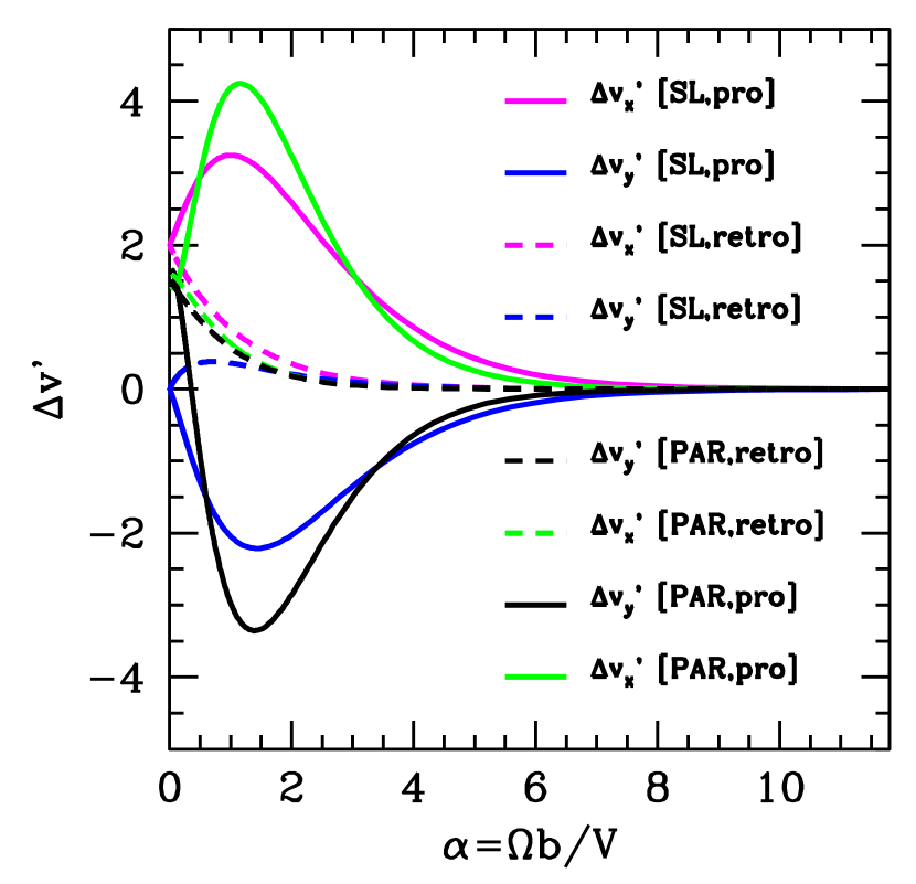
Figure 4.— Velocity increments of stars rotating in a victim while encountering a system on straight line or parabolic orbits. Shown are the quantities $(\Delta\rm{v}_{x})_{\rm{sl}}^{{}^{\prime}}$ and $(\Delta\rm{v}_{y})_{\rm{sl}}^{{}^{\prime}}$ as functions of the parameter $\alpha$ for prograde and retrograde encounters.

Figure 4 shows the velocity perturbations on stars within a spinning disk from either straight-line or parabolic encounters. For the prograde cases, the response is a maximum near $\alpha\sim 1$, where there is a matching between the spin frequency of the rotating victim and the orbital frequency around the perturber,

$$\Omega_{\rm{victim}}=\Omega_{\rm{pert}}\ \ \rightarrow\ \ \frac{v}{r}\sim\frac{V}{R},$$ (86)

characteristic of a resonance. However, the resonance is broad, with FWHM $\Delta\alpha\sim 2$; hence, we refer to this phenomenon as a quasi-resonance.

The width of the resonance can be understood from the fact that, owing to the non-circular nature of the perturber’s orbit, its effective orbital frequency as perceived by the victim changes with time. As a result, the resonance is “maximal” only for a short period of time. Furthermore, at each point along the orbit the instantaneous orbital frequency can be in resonance with stars located at different radii within the victim, and can therefore act more efficiently on different parts of it at different times.

In a true resonant interaction, it is assumed that a periodic perturbation is applied for an indefinite length of time. In that event, the resonance will be narrow because perturbations off-resonance will cancel out in the limit of infinitely many cycles. For a tidal encounter from an unbound trajectory, as we consider here, this is not necessarily the case and off-resonant driving forces can result in a non-zero perturbation. This incomplete cancellation explains why the response for prograde encounters shown in Figure 4 is broad. For retrograde interactions, the cancellation is more complete and the response is suppressed. For both prograde and retrograde cases, in the limit $\alpha\rightarrow\infty$, a star in the victim can complete many orbits while the perturber is near a particular orbital frequency, resulting in an averaging out of the perturbation, yielding an exponentially suppressed response.

Figure 4 also illustrates the maximal response in the different cases for $\alpha\sim$1. Near this value of $\alpha$, the velocity increments owing to the quasi-resonant phenomenon are greater when the victim experiences a parabolic encounter than in the case of a straight line path, since the curvature of the orbit implies that the resonance is applied for a longer time. For non-rotating systems ($\alpha\rightarrow 0$), the velocity increment gained by the stars in the victim is described by the usual impulse approximation. In quasi-resonance, the velocity perturbations in the prograde cases are a factor $\sim 2-3$ higher than in this limit, while the response is suppressed of a similar factor for a retrograde collision for $\alpha\sim 1$.

Note that in our analysis, the disk is assumed to be infinitely thin. However the large resonance width shown in Figure 4 would make the results applicable even to rotating systems with a finite velocity dispersion. Qualitatively we expect that for a “hot” disk victim the resonant response would still occur, although the efficiency will be somewhat reduced.

4. Non-coplanar encounters

In order to generalize the formulation presented earlier to non-coplanar encounters, we need to consider situations where the orbit plane is arbitrarily inclined relative to that of the victim disk. To facilitate interpretation of the results, especially vertical heating of the disk, we choose to perform this operation by actively rotating the orbit plane, leaving the unperturbed disk in the $x-y$ plane. Thus, as above, the coordinates of stars in the victim disk are still given by eq. (2) and the trajectory of the perturber, $\overrightarrow{R}(t)$, will be specified by rotating its coplanar path, which we will refer to as $\overrightarrow{R}_{cop}(t)$ in the following.

To describe the rotation, we introduce the $3\times 3$  matrix $\tilde{A}$, given by:

$$\tilde{A}=\left[\begin{array}[]{ccc}a_{11}&a_{12}&a_{13}\\ a_{21}&a_{22}&a_{23}\\ a_{31}&a_{32}&a_{33}\end{array}\right].$$

Then the rotated trajectory of the encounter is given by

$$\overrightarrow{R}(t)=\tilde{A}\overrightarrow{R}_{cop}(t)\,.$$ (87)

Rotating the path of the perturber does not alter the magnitude of $\overrightarrow{R}(t)$ and so

$$R(t)=\left|\tilde{A}\overrightarrow{R}_{cop}(t)\right|=R_{cop}(t)\,.$$ (88)

The convention for the Euler angles that specify the rotation matrix $\tilde{A}$ is not unique.

Defining

$$\begin{array}[]{cc}c_{\lambda}=\cos\lambda;s_{\lambda}=\sin\lambda\\ c_{\eta}=\cos\eta;s_{\eta}=\sin\eta~{},\\ c_{\chi}=\cos\chi;s_{\chi}=\sin\chi\end{array}$$

we take the rotation matrix to be

$$\tilde{A}=\left[\begin{array}[]{ccc}c_{\lambda}c_{\eta}c_{\chi}-s_{\lambda}s_{\chi}&-c_{\lambda}c_{\eta}s_{\chi}-s_{\lambda}c_{\chi}&c_{\lambda}s_{\eta}\\ s_{\lambda}c_{\eta}c_{\chi}+c_{\lambda}s_{\chi}&-s_{\lambda}c_{\eta}s_{\chi}+c_{\lambda}c_{\chi}&s_{\lambda}s_{\eta}\\ -s_{\eta}c_{\chi}&s_{\eta}s_{\chi}&c_{\eta}\end{array}\right],$$

corresponding to a first rotation about the $z$ axis by an angle $\chi$, a second rotation about the $y$ axis by an angle $\eta$, and a third rotation about the $z$ axis again by an angle $\lambda$. In other words, $\tilde{A}\equiv R(z,~{}\lambda)R(y,~{}\eta)R(z,~{}\chi)$, where $R(x_{i},~{}\theta)$ is a standard matrix describing a rotation by an angle $\theta$ about the $x_{i}$ axis. The angles $\chi$, $\eta$, and $\lambda$ can take arbitrary values (positive or negative), with the sense of rotation determined by the right hand rule. For example, the orbital angular momentum for a coplanar collision is $\overrightarrow{L}_{cop}(t)=L_{orb}\hat{z}$, implying

$$\overrightarrow{L}(t)=\tilde{A}\overrightarrow{L}_{cop}(t)=L_{orb}(\cos\lambda\sin\eta,\sin\lambda\sin\eta,\cos\eta)\,.$$ (89)

4.1. Encounters on straight line paths

We consider first the case of non-coplanar encounters in which the perturber moves along a straight-line, generalizing the results of §3.1. The coplanar trajectory is given by eq. (11), the phase angle of the stars along their orbits in the victim is, as earlier, defined by eq. (12), and we employ the parameter $\alpha$, as defined by eq. (14). Note, however, that now the sign of $\Omega$ does not determine if the encounter is prograde or retrograde, but merely fixes the direction of the spin angular momentum of the victim, either along the $+z$ axis (positive $\Omega$) or $-z$ axis (negative $\Omega$). For non-coplanar collisions, the condition of whether the encounter is mainly prograde versus retrograde is set by $\beta=\overrightarrow{L}(t)\cdot\overrightarrow{S}(t)/(LS)$, where $\overrightarrow{L}(t)$ and $\overrightarrow{S}(t)$ are the orbital angular momentum of the encounter and the spin angular momentum of the victim disk, respectively. The quantity $\beta$ lies between $+1$ (purely prograde) and $-1$ (purely retrograde) and takes the value $\beta=0$ for a polar orbit.

Starting from the expressions for the velocity perturbations in eq. (9) we find, after algebra:

$$\Delta v_{x}=-{{2GM_{pert}}\over{b^{2}V_{sl}}}\,r\,\Biggl{\{} \alpha^{2}K_{0}(\alpha)\left[(a_{12}^{2}-a_{11}^{2})\cos\phi_{0}+(a_{12}a_{22}-a_{11}a_{21})\sin\phi_{0}\right]$$

$$+\,\alpha K_{1}(\alpha)\left[(1-2a_{11}^{2}-a_{12}^{2})\cos\phi_{0}-(a_{12}a_{22}+2a_{11}a_{21})\sin\phi_{0}\right]\,$$

$$\mp\alpha^{2}K_{1}(\alpha)\left[(a_{11}a_{22}+a_{21}a_{12})\cos\phi_{0}-2a_{11}a_{12}\sin\phi_{0}\right]\Biggr{\}}$$ (90)

$$\Delta v_{y}=-{{2GM_{pert}}\over{b^{2}V_{sl}}}\,r\,\Biggl{\{} \alpha^{2}K_{0}(\alpha)\left[(a_{12}a_{22}-a_{11}a_{21})\cos\phi_{0}+(a_{22}^{2}-a_{21}^{2})\sin\phi_{0}\right]\,$$

$$+\,\alpha K_{1}(\alpha)\left[(1-2a_{21}^{2}-a_{22}^{2})\sin\phi_{0}-(a_{12}a_{22}+2a_{11}a_{21})\cos\phi_{0}\right]$$

$$\pm\,\alpha^{2}K_{1}(\alpha)\left[(a_{21}a_{12}+a_{22}a_{11})\sin\phi_{0}-2a_{21}a_{22}\cos\phi_{0}\right]\Biggr{\}}$$ (91)

$$\Delta v_{z}=-{{2GM_{pert}}\over{b^{2}V_{sl}}}\,r\,\Biggl{\{} \alpha^{2}K_{0}(\alpha)\left[(a_{32}a_{12}-a_{31}a_{11})\cos\phi_{0}+(a_{32}a_{22}-a_{31}a_{21})\sin\phi_{0}\right]$$

$$+\,\alpha K_{1}(\alpha)\left[-(a_{32}a_{22}+2a_{31}a_{21})\sin\phi_{0}-(a_{32}a_{12}+2a_{11}a_{31})\cos\phi_{0}\right]$$

$$\pm\,\alpha^{2}K_{1}(\alpha)\left[(a_{31}a_{12}+a_{32}a_{11})\sin\phi_{0}-(a_{31}a_{22}+a_{21}a_{32})\cos\phi_{0}\right]\Biggr{\}}.$$ (92)

Here, the factors $a_{ij}$ are the relevant components of the rotation matrix $\tilde{A}$, and the upper signs in the $\mp$ and $\pm$ terms refer to the case with $\Omega>0$ while the lower signs are for the case with $\Omega<0$. It is straightforward to show that these expressions reduce to the appropriate ones for coplanar encounters given in §3.1 if the rotation angles are set to zero.

As a simple illustration, consider a straight-line path where the original orbit is in the $x-y$ plane and is given by $\overrightarrow{R}_{cop}(t)=(b,V_{sl}\,t,0)$, and employ the Euler angle convention summarized above. Rotate this path by an angle $\eta$ around the $y$-axis, so that

$$\overrightarrow{R}(t)=(b\cos\eta,V_{sl}\,t,-b\sin\eta)\,.$$ (93)

In this case,

$$\overrightarrow{L}(t)=L_{orb}(\sin\eta,0,\cos\eta)\,,$$ (94)

and the components of the rotation matrix are given by

$$\tilde{A}=\left[\begin{array}[]{ccc}\cos\eta&0&\sin\eta\\ 0&1&0\\ -\sin\eta&0&\cos\eta\end{array}\right].$$

Thus, from the equation about for $\Delta v_{z}$, the vertical heating can be estimated as a function of $\eta$ and is

$$\Delta v_{z}=-{{2GM_{pert}}\over{b^{2}V_{sl}}}\,r\cos\phi_{0}\,\Biggl{\{}{1\over 2}\alpha^{2}K_{0}(\alpha)\sin 2\eta\,+\,\alpha K_{1}(\alpha)\sin 2\eta\,\pm\,\alpha^{2}K_{1}(\alpha)\sin\eta\Biggr{\}}.$$ (95)

It is straightforward to show that the dependence on $\eta$ in this expression is such that the response leads to a vertical warping of the disk, with an efficiency depending on $\eta$.

4.2. Parabolic orbits

We now adopt the coplanar trajectory given in eqs. (43) - (47) and apply the rotation matrix $\tilde{A}$ to the orbit. Following a similar procedure as for the straight-line path, the velocity perturbations can be written in the form:

$$\Delta v_{x}=-{{2GM_{pert}}\over{b^{2}V_{0}}}\,r\,\Biggl{\{}\left[2\cos\phi_{0}-3A_{x}\right]I_{20}(\sqrt{2}\alpha)\,-\,3B_{x}I_{22}(\sqrt{2}\alpha)\,-\,3C_{x}I_{2-2}(\sqrt{2}\alpha)\Biggr{\}}$$ (96)

$$\Delta v_{y}=-{{2GM_{pert}}\over{b^{2}V_{0}}}\,r\,\Biggl{\{}\left[2\sin\phi_{0}-3A_{y}\right]I_{20}(\sqrt{2}\alpha)\,-\,3B_{y}I_{22}(\sqrt{2}\alpha)\,-\,3C_{y}I_{2-2}(\sqrt{2}\alpha)\Biggr{\}}$$ (97)

$$\Delta v_{z}=-{{2GM_{pert}}\over{b^{2}V_{0}}}\,r\,\Biggl{\{}-3A_{z}I_{20}(\sqrt{2}\alpha)\,-\,3B_{z}I_{22}(\sqrt{2}\alpha)\,-\,3C_{z}I_{2-2}(\sqrt{2}\alpha)\Biggr{\}}\,,$$ (98)

where the terms $A_{x},A_{y},A_{z},B_{x},B_{y},B_{z},C_{x},C_{y}$, and $C_{z}$ are given by:

$$A_{x}=(a_{11}^{2}+a_{12}^{2})\cos\phi_{0}\,+\,(a_{11}a_{21}+a_{21}a_{22})\sin\phi_{0}$$ (99)

$$B_{x}={1\over 2}\left[(a_{11}^{2}-a_{12}^{2}\mp a_{11}a_{22}\mp a_{21}a_{12})\cos\phi_{0}\,+\,(a_{11}a_{21}-a_{12}a_{22}\pm 2a_{11}a_{12})\sin\phi_{0}\right]$$ (100)

$$C_{x}={1\over 2}\left[(a_{11}^{2}-a_{12}^{2}\pm a_{11}a_{22}\pm a_{21}a_{12})\cos\phi_{0}\,+\,(a_{11}a_{21}-a_{12}a_{22}\mp 2a_{11}a_{12})\sin\phi_{0}\right]$$ (101)

$$A_{y}=(a_{12}a_{22}+a_{11}a_{21})\cos\phi_{0}\,+\,(a_{21}^{2}+a_{22}^{2})\sin\phi_{0}$$ (102)

$$B_{y}={1\over 2}\left[(a_{11}a_{21}-a_{12}a_{22}\mp 2a_{21}a_{22})\cos\phi_{0}\,+\,(a_{21}^{2}-a_{22}^{2}\pm a_{12}a_{21}\pm a_{22}a_{11})\sin\phi_{0}\right]$$ (103)

$$C_{y}={1\over 2}\left[(a_{11}a_{21}-a_{12}a_{22}\pm 2a_{21}a_{22})\cos\phi_{0}\,+\,(a_{21}^{2}-a_{22}^{2}\mp a_{12}a_{21}\mp a_{22}a_{11})\sin\phi_{0}\right]$$ (104)

$$A_{z}=(a_{32}a_{12}+a_{11}a_{31})\cos\phi_{0}\,+\,(a_{32}a_{22}+a_{31}a_{21})\sin\phi_{0}$$ (105)

$$B_{z}={1\over 2}\left[(a_{11}a_{31}-a_{32}a_{12}\mp a_{31}a_{22}\mp a_{32}a_{21})\cos\phi_{0}\,+\,(a_{31}a_{21}-a_{32}a_{22}\pm a_{31}a_{12}\pm a_{32}a_{11})\sin\phi_{0}\right]$$ (106)

$$C_{z}={1\over 2}\left[(a_{11}a_{31}-a_{32}a_{12}\pm a_{31}a_{22}\pm a_{32}a_{21})\cos\phi_{0}\,+\,(a_{31}a_{21}-a_{32}a_{22}\mp a_{31}a_{12}\mp a_{32}a_{11})\sin\phi_{0}\right].$$ (107)

As earlier, the factors $a_{ij}$ are the relevant components of the rotation matrix $\tilde{A}$, and the upper signs in the $\mp$ and $\pm$ terms refer to the case with $\Omega>0$ while the lower signs are for the case with $\Omega<0$. In particular, whether the encounter is mainly prograde or retrograde is set by the sign of $\beta$, as given above.

In the equations for $\Delta v_{k}$, the functions $I_{22}$ and $I_{2-2}$ can be simplified to expressions involving $I_{l0}$ using the recursion relations eqs. (61) and (62).

5. Numerical Experiments

To test the reliability of the quasi-resonant approximation, we carry out simulations of encounters between a spinning system and an external perturber passing either on a straight line path or a parabolic orbit. For simplicity, we adopt a restricted three-body method for following the development of tidal tails during collisions. The restricted three-body scheme is appropriate for this application because the formation of tidal tails is essentially a kinematic process (Dubinski et al., 1999).

In our experiments, the victim is a point mass surrounded by a flat annular disk of test particles. Initially, the particles are on circular, Keplerian orbits around the central point mass. We employ a system of units in which Newton’s constant, $G$, and the maximum radius and mass of the victim are all set equal to unity.

For each victim, we place test particles on 400 annuli surrounding the point mass. The annuli are linearly spaced in radius, between $r_{\rm min}=0.05$ and $r_{\rm max}=1$ around the central mass point with a total number of approximately 1.3$\times$10⁵ particles. The annuli have an angular spacing such that the particles are equidistantly distributed along each ring, with a spacing $\Delta l=0.01=r\Delta\phi$. This choice ensures a fair sampling of the outermost rings, a better visual comparison, and an accurate sampling of the energy distribution of the stars in the victim. The perturber is modeled as a point mass passing either on a straight line or parabolic orbit. In this way, the problem of the encounter is restricted to a three-body problem since each test particle (“star”) feels only the gravitational force from the massive particles (the central point mass of the victim and the perturber). We evolve the models for many dynamical times and compute the energy distribution of the particles long after the passage of the perturber, at a time where the energy configuration of the system reaches a steady state. These estimates are compared to analytical estimates using the approximations presented earlier.

The comparison to the quasi-resonant impulse gained from each star in the victim is done as follows. We mimic the effect of encounters by setting up the victim as a point mass surrounded by a flat annular disk of particles. We then assign to each test particle a circular, Keplerian velocity plus a velocity increment estimated from the analytic approximation for a given perturber mass and impact parameter, and allow the disk to evolve. The total energy of individual test particles is thus always conserved. While our formalism can describe encounters of any mass ratio, we focus here on equal mass situations with $M_{pert}=M_{victim}=1$, and an impact parameter $b$=2, which is twice as large as our disk of test particles. For the straight line case, the choice of the relative velocity $V_{sl}$ is arbitrary, so first we test our approximations for a fast encounter (i.e. a weak perturbation), which is the case where our formalism is expected to be most accurate. In addition, we test the validity of the approximations for slow encounters, which characterize stronger perturbations that are less impulsive.

In what follows, we present numerical tests of coplanar, straight line encounters with fast and slow relative velocities, as well as parabolic encounters at linear and second order approximations. The non-coplanar case has been also tested to ensure that our analytic formulation is reasonable, but for brevity we present results only for co-planar encounters. More general tests of the validity of our analytic treatment will be considered in due course in applications to observed systems.

5.1. Results

Figure 5 gives a visual comparison of the evolution of a victim under the tidal influence of the fast passage of a perturber on a straight line with relative velocity $V_{sl}$=7.5. The top panels illustrate the system with test particles kicked by velocity increments according to the quasi-resonant approximation described in the previous sections. The bottom panels display the evolution of the victim when an external perturber passes close to the disk using a restricted three-body treatment. Figures 5-6 illustrate a coplanar prograde encounter, while the corresponding retrograde coplanar case is displayed in Figures 7-8. Colors are assigned to rings according to their initial distance from the central point mass.

First, as expected, tails are produced for prograde encounters (Figure 5), but are suppressed in retrograde cases (Figure 7). The visual agreement in the extents and shapes of the tails between the analytic (upper panels) and the numerical (lower panels) approaches is good. Further insight is provided by comparing the distribution of specific energies of the disk particles as shown in Figures 6 and Figure 8 for the prograde and retrograde cases, respectively. The different panels show the time evolution of the specific energies for the restricted three-body simulation (blue) and the analytic calculation (red), which is static.

Fast encounters correspond to relatively modest tidal perturbations, leading to a weak resonant response. The amount of energy transferred during the encounter is small and the resulting tails are less spatially extended than ones produced for stronger tidal perturbations (see Figure 9, discussed below). As expected, prograde and retrograde encounters lead to very different energy distributions, since prograde encounters transfer much more energy to the victim than retrograde ones, producing much more massive tails in the prograde case, as demonstrated in Figures 5 and 7. Indeed, according to our analytic results the maximum resonant response is obtained for rings placed at distances corresponding to the parameter $\alpha\sim 1$ (Figure 4). In this particular example, the outermost rings which contribute significant material to the tails are only weakly resonant because their spin frequencies are such that they have a value of $\alpha\sim 0.2-0.3$. Note that our lowest-order approximations yield symmetric tails as shown in the top panels of Figure 5, whereas the numerical simulation yields tails that are slightly asymmetric (bottom panels in Figure 5). This effect increases for stronger perturbations, and is connected to higher order corrections as described in the sections above.

For retrograde encounters, the orbital and spin angular momenta are misaligned and, as shown in Figure 8 for the evolution of the energy distribution, little energy is transferred during the encounter. A resonance does not develop and tail formation is suppressed, as shown in Figure 7.

The quasi-resonant approximation at lowest order, eq. (9), becomes less accurate for slow encounters, where the tidal forces are less impulsive and where the effective duration of the encounter is of the order of the dynamical time of the particles (“stars”) in the outermost rings. Indeed, this is the case where the restricted three-body simulation shows that some mass from the victim is captured by the perturber, introducing a large asymmetry and greater changes in the energy configuration of the final system. The lack of symmetry in tail-making owes to non-linear effects. We can account for some of these by including the next order correction to the response, as given by eqs. (38-39) and eqs. (78-79) for the straight-line and parabolic cases, respectively. We emphasize, however, that even when we include these corrections we assume that stars in the victim move along unperturbed orbits throughout the course of the encounter, thereby treating the orbital variations as small and implicitly ignoring the non-linear response.

Figure 9 shows a prograde straight-line encounter for the relative velocity $V_{sl}=1.5$, as predicted by our analytic approximation when the second order correction is included in the evaluation of the velocity increments given to the disk particles (top panels). This evolution is compared to a simulation with the same disk perturbed by an external body (bottom panels). As noted above, the tail connecting the victim to the perturber is not reproduced by our analytic formalism in detail because we ignore the non-linear response of the victim during the encounter. Nevertheless, the trailing tail, displayed in the region of the plane with $y<0$, is similar in shape and orientation to the one generated in the restricted three-body simulation. Indeed our analytic expression predicts the correct shape of the tail, although it is slightly more extended compared to the one in the actual simulation. The energy distribution of the particles contained in the trailing tail in both models is shown in Figure 10, where the energy is shown in a logarithmic scale. Allowing for the fact that our analytic method cannot entirely account for non-linear effects, we find the comparison encouraging. Indeed, as the energy scale in Figure 10 is logarithmic, the regions showing obvious disagreement contain few stars.

Next, we show an encounter from a parabolic trajectory where the relative velocity of victim and perturber at closest approach is $V_{0}=1.4$ for the parameters adopted in the numerical experiments. Figure 11 shows a prograde parabolic encounter as predicted by our analytic approximation when the second order correction is included in the evaluation of the velocity increments (top panels). The evolution is compared to a restricted three-body simulation with the same disk as perturbed by an external body passing on a parabolic trajectory (bottom panels). This encounter, as well as the slow straight line case, leads to strong resonant effects. In fact, the parameter $\alpha$, for both cases, is around 1.3 for the outermost ring. Hence these rings should have a near-maximal response. This is demonstrated in Figure 11, which shows longer tails as compared to the fast, straight-line encounter. The asymmetry is also reflected in the energy distribution of the slow straight-line encounter (Figure 10) and of the parabolic case (Figure 12) which appear to be bimodal.

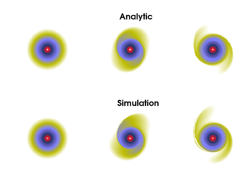
Figure 5.— Time evolution of the victim in the x-y plane under the tidal effect of a fast perturber passing on a straight-line path on a prograde coplanar orbit. The upper left panel illustrates the initial set up where test particles in the annuli are kicked by velocity increments according to the quasi-resonant approximation to linear order, as described in the text. Time evolves from left to right. Bottom panels show the evolution in time of the victim (from the initial set up on the left to the final appearance of tails to the right) when an external perturber is passing on a straight line path, in a restricted three-body simulation. The external perturber passes to the right side of the victim. Colors are assigned to rings according to their initial distance from the central point mass. The left panel shows the initial conditions, the middle panel is the system at time 3.5 and the right panel is the system at time 9.75.

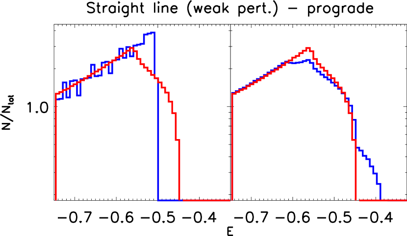
Figure 6.— Time evolution of the energy distribution of the stars of the victim long after the passage of the perturber on a fast straight-line path. The energy of the victim particles in a simulation when an external perturber is involved (blue solid lines) is compared to the energy distribution predicted by the quasi-resonant approximation to linear order (red solid lines). In particular the red solid line is a setup of stars on Keplerian orbits with an (initial) velocity distribution assigned according to the increment to the particle velocity given from our approximations. Note that the two red curves on the left and on the right panel are identical since the energy of each test particle is strictly conserved along its orbit in this case. The left panel shows the initial conditions and the right panel is the system at time 9.75. The time of closest approach in the simulation is 2.

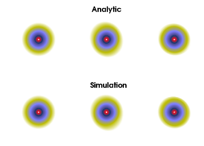
Figure 7.— Time evolution of the victim in the x-y plane under the tidal effect of a perturber passing on a straight-line path on a retrograde coplanar orbit. Top and bottom panels are as in Figure 5. The left panel shows the initial conditions, the middle panel is the system at time 3.5 and the right panel is the system at time 9.75.

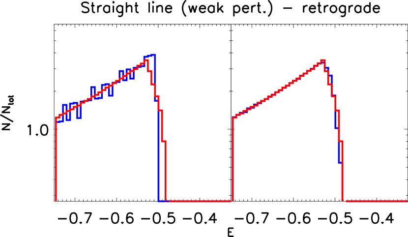
Figure 8.— Time evolution of the energy distribution of the stars in the victim long after the passage of the perturber on a fast straight-line path on a retrograde orbit. The energy distribution of the particles perturbed by the linear order tidal approximation is shown by the red solid lines, whereas the simulation with an external perturber is represented by the blue solid lines. The left panel shows the initial conditions and right panel is the system at time 9.75. The time of closest approach is 2.

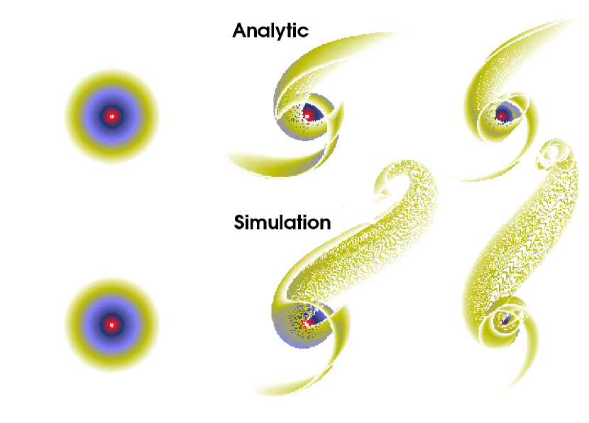
Figure 9.— Time evolution of the victim under the tidal effect of a slow perturber passing on a straight line path. The orbit is prograde. Top and bottom panels are as in Figure 5. The left panel shows the initial conditions, the middle panel is the system at time 10.75 and the right panel is the system at time 30.

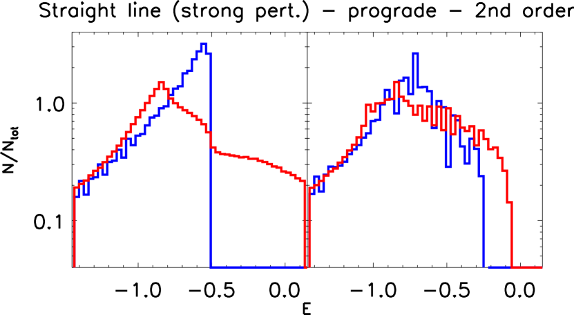
Figure 10.— Time evolution of the energy distribution of stars in the victim long after the passage of a perturber on a slow straight line path on a prograde orbit. The energy distribution of the particles perturbed by the second order tidal approximation is shown by the red solid lines, whereas the restricted three-body simulation of an encounter with an external perturber is represented by the blue solid lines. Since the distributions only involve the particles in the trailing tails (y$<$0 in the x-y plane) the two red solid curves on the left and on the right panel are not identical. The left panel shows the initial conditions and the right panel is the system at time 30. The time of closest approach in the simulation is 10.

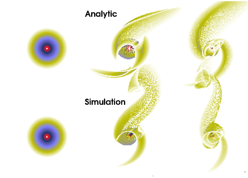
Figure 11.— Time evolution of the victim under the tidal effect of a perturber passing on a prograde coplanar parabolic orbit. Top and bottom panels are as in Figure 5.

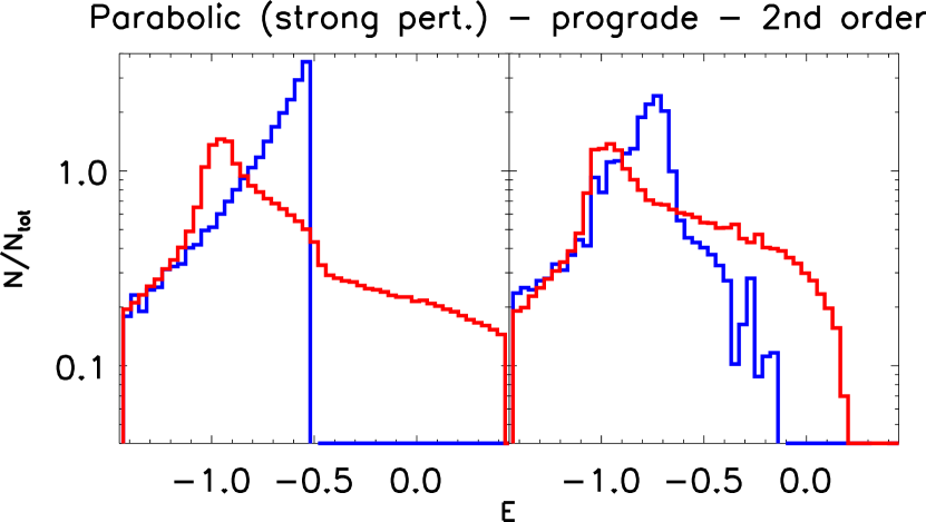
Figure 12.— Time evolution of the energy distribution of stars in the victim long after the passage of a perturber on a parabolic trajectory on a prograde orbit. The energy distribution of the particles using the analytical approximation to second order is shown by the red solid lines, whereas the encounter with an external perturber is represented by the blue solid lines. Since the distributions only involve the particles in the trailing tails (y$<$0 in the x-y plane) the two red solid curves on the left and on the right panel are not identical.

6. Conclusions

We have formulated a simple analytic theory describing the resonant response of rotating objects to gravitational tidal perturbations. We estimated the velocity perturbations on a spinning disk resulting from an encounter with a system on either a straight-line or a parabolic orbit. Our main conclusions are the following:

• The resonant phenomenon described here is an incomplete or “quasi-” resonant process because the perturbation is applied at a given frequency for only a finite period of time. Consequently, the resonance is broad and is maximal when the spin frequency of the rotating victim matches the peak orbital frequency of the encounter. The resonance is broad because the perturbation at each frequency is not applied over many cycles, as for a strictly periodic forcing, so perturbations at slightly off-resonant frequencies do not cancel out completely. However, because the resonance is broad, at each point along the orbit the orbital frequency can be in resonance with parts of the victim disk located at different radii and can therefore act on various locations in the disk at different times. This feature is interesting for galaxy encounters because it means that the victim can loose baryonic mass from different points in the disk by resonant stripping at various times, making the “quasi-resonant” response more damaging than if only certain regions in the disk were being affected.

• In the quasi-resonant regime, the velocity increments gained by the stars in the victim are greater during a parabolic encounter than in the case of a straight-line interaction. For non-rotating systems, the velocity perturbations are described by the usual impulse approximation. In prograde cases (both straight or parabolic) the velocity perturbations owing to quasi-resonant phenomenon are at least factor $\sim 2$ higher than in the impulse approximation while the response is suppressed for retrograde encounters.

• When compared to numerical simulations we find that the quasi-resonant approximation provides a simple physical model for describing the nature of the tails in interacting disk galaxies and gives well-defined and reasonable values for the changes in velocities as a result of tidal encounters. In particular, the quasi-resonant approximation gives accurate results for high speed encounters, where the effective duration of the encounter is less than or of order the dynamical time of the particles (“stars”) of the spinning system. The main reason is that high velocity encounters generate small perturbations of otherwise steady-state systems and keep them in the linear regime, where the analytic approximation is valid. The quasi-resonant approximation is less accurate for slower encounters, where the tidal forces act over a longer period of time. This is particularly true for the case of a perturber passing on a parabolic trajectory. Indeed, in these events the numerical simulations show that some mass of the victim galaxy is captured by the perturber. However, a better match can be obtained by including higher order corrections for the velocity perturbations in the analytic formalism.

• The lengths of the tails depends on the amount of energy transferred to the victim during an encounter. Prograde encounters with more massive perturbers pump larger amounts of energy into the victims, yielding more extended tails but also introducing asymmetries with the leading tails being more elongated than the trailing ones. Retrograde encounters transfer much less energy into the victim, suppressing the development of tails.

Finally, we note that our findings for tail-making during galaxy-galaxy encounters may apply to gas as well. Thus, our calculations may be used to understand the geometry of the gas streams and bridges of stars associated with dwarf galaxies, as recently discovered in the Panda survey of M31 (McConnachie et al., 2009). Other potential applications include warps and heating of galactic disks by tidal perturbations, understanding the conditions for long tails to be produced in galaxy collisions depending on the dark matter distribution in the halos, and identifying situations where stars can be unbound in galaxy interactions and be ejected into the intergalactic medium or populate the field of groups and clusters. Moreover, our theory may be relevant to other applications, such as to studies of the stability of binary stars perturbed by a third body or to investigations of protoplanetary disks perturbed by close passages of stars.

Appendix A Generalized Airy functions

Our analysis of parabolic tidal encounters results in expressions that involve the generalized Airy functions of Press & Teukolsky (1977), defined by eq. (58). The first one, $I_{00}$, is a modified Bessel function or (conventional) Airy function,

$$I_{00}(\sqrt{2}\alpha)=3^{-1/2}K_{1/3}\Big{(}2^{3/2}\frac{\sqrt{2}\alpha}{3}\Big{)}=\pi(2\alpha)^{-1/3}\rm{Ai}[(2\alpha)^{2/3}]\,.$$ (A1)

Press & Teukolsky (1977) provide the following rational function approximations to $I_{10},~{}I_{20},$ and $I_{30}$, making it possible to straightforwardly estimate the velocity perturbations in a parabolic tidal encounter:

$$I_{10}(y)=\frac{1.5288+0.79192\sqrt{y}-0.86606y+0.14593y\sqrt{y}}{1.+1.6449\sqrt{y}-1.2345y+0.19392y\sqrt{y}}e^{-\frac{2^{3/2}}{3}y},\ \ \ \ \ \ \ \ \ \ \ \ \rm{for}\ \ y\ \ \leq 4\ \ \ \ \ \ \ \ \$$ (A2)

$$I_{10}(y)=\frac{1.4119+18.158\sqrt{y}+22.152y}{1.+12.249\sqrt{y}+28.593y}e^{-\frac{2^{3/2}}{3}y},\ \ \ \ \ \ \ \ \ \ \ \ \ \ \ \ \rm{for}\ \ y\ \ \geq 4\ \ \ \ \ \ \ \ \ \$$ (A3)

$$I_{20}(y)=\frac{0.78374+1.5039\sqrt{y}+1.0073y+0.71115y\sqrt{y}}{1.+1.9128\sqrt{y}+1.0384y+1.2883y\sqrt{y}}\Big{(}1+\frac{2^{3/2}}{3}y\Big{)}^{1/2}e^{-\frac{2^{3/2}}{3}y},\ \ \ \ \ \ \ \ \ \$$ (A4)

$$I_{30}(y)=\frac{0.58894+0.32381\sqrt{y}+0.45605y+0.15220y\sqrt{y}}{1.+0.54766\sqrt{y}+0.76130y+0.53016y\sqrt{y}}\Big{(}1+\frac{2^{3/2}}{3}y\Big{)}e^{-\frac{2^{3/2}}{3}y}.\ \ \ \ \ \ \ \ \ \$$ (A5)

These expressions are accurate to around $\leq 0.1$%, except for very small and very large values of $\alpha$, where the error rises to a few percent.

To evaluate the limit $\alpha\to\infty$ of the parabolic encounter case studied in this work, it is necessary to know the asymptotic behavior of the generalized Airy functions as $y\to\infty$. In what follows, we give these asymptotic expansions and outline the key steps of their derivation. While the $l=0$ case corresponds to the usual Airy function, the $l=1,~{}2,~{}3$ cases have not been extensively studied before, and the numerical fits provided by Press & Teukolsky (1977) are not sufficiently accurate to capture exact cancellations in the results. Ostriker (1994) previously calculated these asymptotic expansions to leading order using similar techniques, but some of the limits we take involve exact cancellations at this order, so that it is necessary to compute higher-order terms.

The starting point for the asymptotic expansions is the integral expression (eq. 58)

$$I_{l0}(y)=\int_{0}^{\infty}(1+\xi^{2})^{-l}\cos{[\sqrt{2}y(\xi+\xi^{3}/3)]}d\xi.$$ (A6)

The main technical difficulty in determining the asymptotic behavior of $I_{l0}(y)$ arises from the fact that the cosine term oscillates extremely rapidly as $y\to\infty$, and that the value of the integral depends on exactly how the positive and negative parts cancel each other. It is however possible to circumvent this difficulty by expressing equation (A6) in terms of a contour integral in the complex plane, and by using the method of steepest descent (e.g., Bender & Orszag, 1978).

Specifically, we note that

$$I_{l0}(y)=\frac{1}{2}{\rm Re}\left\{\int_{-\infty}^{\infty}(1+\xi^{2})^{-l}\exp{[i\sqrt{2}y(\xi+\xi^{3}/3)]}d\xi\right\}$$ (A7)

and consider the integration contour shown in Figure 13. Making the change of variable $s\equiv i\xi$, the integral within the curly brackets is seen to be equal to an equivalent integral along the imaginary axis:

$$-i\int_{-i\infty}^{i\infty}(1-s^{2})^{-l}\exp{[\sqrt{2}y(s-s^{3}/3)]}ds.$$ (A8)

Writing the complex integrand as $f(s)$, the residue theorem implies that $\oint_{C}f(s)ds=2\pi i\sum_{k=1}^{n}{\rm Res}(f,~{}a_{k})$, where the $a_{k}$ are the poles within $C=C_{1}+C_{2}+C_{3}+C_{4}$. Since the integrands along $C_{2}$ and $C_{4}$ are exponentially suppressed in modulus, $\int_{C_{2},C_{4}}f(s)ds\to 0$ as the contour is expanded to infinity, yielding

$$\int_{C_{1}}f(s)ds=-\int_{C_{3}}f(s)ds+2\pi i\sum_{k=1}^{n}{\rm Res}(f,~{}a_{k}).$$ (A9)

As the left hand side is simply related to equation (A8) by the multiplicative factor $-i$, the problem is essentially reduced to evaluating $\int_{C_{3}}f(s)ds$.

The key is to choose the path $C_{3}$ so that the integral is tractable in the limit $y\to\infty$. According to the method of steepest descent, the integral will in this limit receive most of its contribution in the neighborhood of a saddle point, if the integration path is chosen to follow the direction of steepest descent of the exponential argument. Setting $d[s-s^{3}/3]/ds=0$, the relevant saddle point is found to be $s=-1$, and we may parametrize the path of steepest descent by

$$s-s^{3}/3=-2/3-t^{2},~{}t\in(-\infty,\infty),$$ (A10)

chosen so that $s=-1$ at $t=0$. Then,

$$\int_{C_{3}}f(s)ds=\int_{-\infty}^{\infty}f(s(t))\frac{ds}{dt}dt=\exp{\left(-\frac{2^{3/2}}{3}y\right)}\int_{-\infty}^{\infty}\exp{\left(-\sqrt{2}yt^{2}\right)}\frac{1}{[1-s(t)^{2}]^{l}}\frac{ds}{dt}dt,$$ (A11)

provided that the parametrization $s(t)$ is oriented in the same sense as $C_{3}$. Once an explicit expression for $s(t)$ is obtained by solving the cubic equation (A10), we expand the product $[1-s(t)^{2}]^{-l}(ds/dt)$ in a Taylor series around $t=0$. For instance, the $l=0$ case yields $ds/dt=i-(5i/24)it^{2}+(385i/3456)t^{4}+...~{}+$ purely real terms, where the purely real terms do not enter in the final result. The integral on the right hand side of equation (A11) becomes a term-by-term sum of simple Gaussian integrals of the form $b_{n}\int_{-\infty}^{\infty}t^{n}\exp{\left(-\sqrt{2}yt^{2}\right)}dt$, where $n=0,~{}1,~{}2,~{}3,~{}...$ and the $b_{n}$ coefficients are determined by the Taylor expansion. These integrals are easily evaluated and we thus obtain an analytic expansion for $\int_{C_{3}}f(s)ds$ valid in the limit $y\to\infty$.

This procedure can be carried out as described for $l=0$. In this case, there is no residue and we find

$$I_{00}(y)\sim\frac{\sqrt{\pi}}{2^{5/4}}\exp{\left(-\frac{2^{3/2}}{3}y\right)}\left[\frac{1}{y^{1/2}}-\frac{5}{48\sqrt{2}}\frac{1}{y^{3/2}}+\frac{385}{9216}\frac{1}{y^{5/2}}+O\left(\frac{1}{y^{7/2}}\right)\right],$$ (A12)

in agreement with the known result for the ordinary Airy function. For $l>0$, we however encounter the difficulty that the saddle point $s=-1$ is also a pole of order $l$.

For the simple pole of the case $l=1$, the basic procedure remains valid but we must account for the ${\rm Res}(f,-1)$ contribution in equation (A9). Since the pole is located directly on the contour (rather than contained within it) it contributes only half of its value, namely $\pi i\times{\rm Res}(f,-1)$ rather than $2\pi i\times{\rm Res}(f,-1)$, as can be shown by considering infinitesimally modified contours that avoid and enclose the pole. We find ${\rm Res}(f,-1)=(1/2)\exp{[-(2^{3/2}/3)y]}$ and

$$I_{10}(y)\sim\frac{\pi}{4}\exp{\left(-\frac{2^{3/2}}{3}y\right)}\left[1+\frac{2^{3/4}}{3\sqrt{\pi}}\frac{1}{y^{1/2}}-\frac{47}{216\times 2^{3/4}\sqrt{\pi}}\frac{1}{y^{3/2}}+O\left(\frac{1}{y^{5/2}}\right)\right].$$ (A13)

For the $l=2$ and $l=3$ cases, the procedure yields divergent integrals. These can however be avoided by going back to equation (A8) and using a combination of integration by parts and partial fraction expansions to rewrite it in terms of $I_{00}(y)$, $I_{10}(y)$, and other integrals that are regular at $s=-1$ and everywhere within $C$. The latter integrals can then be evaluated in the limit $y\to\infty$ using the method of steepest descent, in close analogy to the $l=0$ case. We finally find:

$$I_{20}(y)\sim\exp{\left(-\frac{2^{3/2}}{3}y\right)}\left[\frac{\pi}{8}+\frac{23\sqrt{\pi}}{192\times 2^{1/4}}\frac{1}{y^{1/2}}+\frac{2869\sqrt{\pi}}{55296\times 2^{3/4}}\frac{1}{y^{3/2}}+O\left(\frac{1}{y^{5/2}}\right)\right]$$ (A14)

and

$$I_{30}(y)\sim\exp{\left(-\frac{2^{3/2}}{3}y\right)}\left[\frac{\pi}{8\times 2^{1/2}}y+\frac{\sqrt{\pi}}{3\times 2^{3/4}}y^{1/2}+\frac{3\pi}{32}+O\left(\frac{1}{y^{1/2}}\right)\right].$$ (A15)

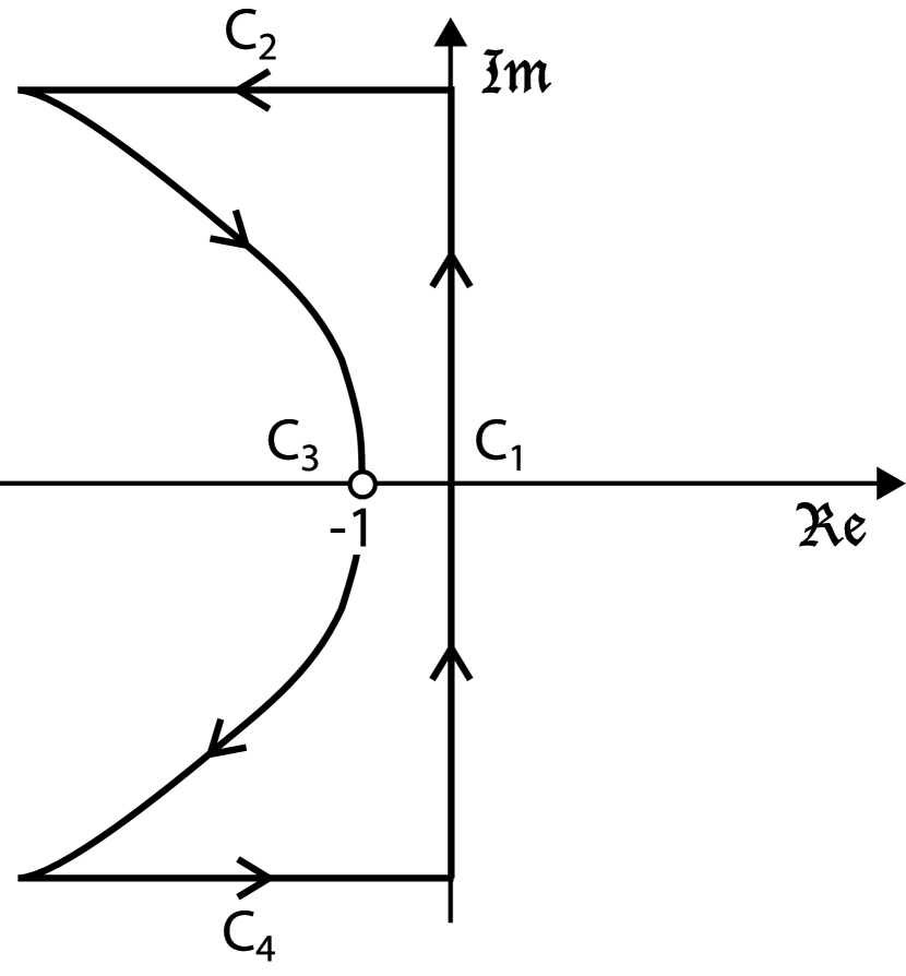
Figure 13.— Integration contour used in the asymptotic expansions of the generalized Airy functions $I_{l0}(y)$ for $y\to\infty$. $C_{3}$ corresponds to the path of steepest descent through the saddle point $s=-1$ of the integral in equation (A8). The method of steepest descent stipulates that most of the contribution to the integral along this path comes from the neighborhood of this saddle point as $y\to\infty$. Using the residue theorem, the desired integrals along the imaginary axis ($C_{1}$) can be evaluated asymptotically.

References

- Abramowitz & Stegun (1972) Abramowitz, M., & Stegun, I. A. 1972, Handbook of Mathematical Functions, ed. I. A. Abramowitz, M. & Stegun
- Aguilar & White (1985) Aguilar, L. A., & White, S. D. M. 1985, ApJ, 295, 374
- Arp (1966) Arp, H. 1966, ApJS, 14, 1
- Barnes (1988) Barnes, J. E. 1988, ApJ, 331, 699
- Barnes (1992) —. 1992, ApJ, 393, 484
- Barnes & Hibbard (2009) Barnes, J. E., & Hibbard, J. E. 2009, AJ, 137, 3071
- Bender & Orszag (1978) Bender, C. M., & Orszag, S. A. 1978, Advanced Mathematical Methods for Scientists and Engineers, ed. Bender, C. M. & Orszag, S. A.
- Besla et al. (2007) Besla, G., Kallivayalil, N., Hernquist, L., Robertson, B., Cox, T. J., van der Marel, R. P., & Alcock, C. 2007, ApJ, 668, 949
- Besla et al. (2010) Besla, G., Kallivayalil, N., Hernquist, L., van der Marel, R. P., Cox, T. J., & Kereš, D. 2010, ApJ, 721, L97
- Binney & Tremaine (1987) Binney, J., & Tremaine, S. 1987, Galactic dynamics, ed. S. Binney, J. & Tremaine
- Choi et al. (2009) Choi, J., Weinberg, M. D., & Katz, N. 2009, MNRAS, 400, 1247
- Clutton-Brock (1972a) Clutton-Brock, M. 1972a, Ap&SS, 17, 292
- Clutton-Brock (1972b) —. 1972b, Ap&SS, 16, 101
- Dekel et al. (1980) Dekel, A., Shaham, J., & Lecar, M. 1980, ApJ, 241, 946
- D’Onghia et al. (2009) D’Onghia, E., Besla, G., Cox, T. J., & Hernquist, L. 2009, Nature, 460, 605
- D’Onghia & Lake (2008) D’Onghia, E., & Lake, G. 2008, ApJ, 686, L61
- D’Onghia et al. (2010) D’Onghia, E., Springel, V., Hernquist, L., & Keres, D. 2010, ApJ, 709, 1138
- Dubinski et al. (1996) Dubinski, J., Mihos, J. C., & Hernquist, L. 1996, ApJ, 462, 576
- Dubinski et al. (1999) —. 1999, ApJ, 526, 607
- Dyson (1987) Dyson, J. 1987, Ap&SS, 139, 196
- Eneev et al. (1973) Eneev, T. M., Kozlov, N. N., & Sunyaev, R. A. 1973, A&A, 22, 41
- Gallagher & Ostriker (1972) Gallagher, III, J. S., & Ostriker, J. P. 1972, AJ, 77, 288
- Hernquist (1992) Hernquist, L. 1992, ApJ, 400, 460
- Hernquist (1993) —. 1993, ApJ, 409, 548
- Hernquist & Quinn (1987) Hernquist, L., & Quinn, P. J. 1987, ApJ, 312, 17
- Hernquist & Spergel (1992) Hernquist, L., & Spergel, D. N. 1992, ApJ, 399, L117
- Hibbard & Mihos (1995) Hibbard, J. E., & Mihos, J. C. 1995, AJ, 110, 140
- Julian & Toomre (1966) Julian, W. H., & Toomre, A. 1966, ApJ, 146, 810
- Kallivayalil et al. (2006) Kallivayalil, N., van der Marel, R. P., & Alcock, C. 2006, ApJ, 652, 1213
- Malin & Carter (1980) Malin, D. F., & Carter, D. 1980, Nature, 285, 643
- Mayer et al. (2002) Mayer, L., Moore, B., Quinn, T., Governato, F., & Stadel, J. 2002, MNRAS, 336, 119
- McConnachie et al. (2009) McConnachie, A. W., Irwin, M. J., Ibata, R. A., Dubinski, J., Widrow, L. M., Martin, N. F., Côté, P., Dotter, A. L., Navarro, J. F., Ferguson, A. M. N., Puzia, T. H., Lewis, G. F., Babul, A., Barmby, P., Bienaymé, O., Chapman, S. C., Cockcroft, R., Collins, M. L. M., Fardal, M. A., Harris, W. E., Huxor, A., Mackey, A. D., Peñarrubia, J., Rich, R. M., Richer, H. B., Siebert, A., Tanvir, N., Valls-Gabaud, D., & Venn, K. A. 2009, Nature, 461, 66
- Mihos et al. (1998) Mihos, J. C., Dubinski, J., & Hernquist, L. 1998, ApJ, 494, 183
- Mirabel et al. (1991) Mirabel, I. F., Lutz, D., & Maza, J. 1991, A&A, 243, 367
- Ostriker (1994) Ostriker, E. C. 1994, ApJ, 424, 292
- Pfleiderer & Siedentopf (1961) Pfleiderer, J., & Siedentopf, H. 1961, Zeitschrift fur Astrophysik, 51, 201
- Press & Teukolsky (1977) Press, W. H., & Teukolsky, S. A. 1977, ApJ, 213, 183
- Quinn (1984) Quinn, P. J. 1984, ApJ, 279, 596
- Read et al. (2006) Read, J. I., Wilkinson, M. I., Evans, N. W., Gilmore, G., & Kleyna, J. T. 2006, MNRAS, 366, 429
- Spitzer (1958) Spitzer, L. J. 1958, ApJ, 127, 17
- Springel & White (1999) Springel, V., & White, S. D. M. 1999, MNRAS, 307, 162
- Toomre & Toomre (1972) Toomre, A., & Toomre, J. 1972, ApJ, 178, 623
- Weinberg (2000) Weinberg, M. D. 2000, ApJ, 532, 922
- Wright (1972) Wright, A. E. 1972, MNRAS, 157, 309
- Yabushita (1971) Yabushita, S. 1971, MNRAS, 153, 97