Absolute determination of the ²²Na($p,\gamma$)²³Mg reaction rate in novae

Abstract

Gamma-ray telescopes in orbit around the Earth are searching for evidence of the elusive radionuclide ²²Na produced in novae. Previously published uncertainties in the dominant destructive reaction, ²²Na($p,\gamma)^{23}$Mg, indicated new measurements in the proton energy range of 150 to 300 keV were needed to constrain predictions. We have measured the resonance strengths, energies, and branches directly and absolutely by using protons from the University of Washington accelerator with a specially designed beamline, which included beam rastering and cold vacuum protection of the ²²Na implanted targets. The targets, fabricated at TRIUMF-ISAC, displayed minimal degradation over a $\sim$ 20 C bombardment as a result of protective layers. We avoided the need to know the absolute stopping power, and hence the target composition, by extracting resonance strengths from excitation functions integrated over proton energy. Our measurements revealed that resonance strengths for $E_{p}$ = 213, 288, 454, and 610 keV are stronger by factors of 2.4 to 3.2 than previously reported. Upper limits have been placed on proposed resonances at 198-, 209-, and 232-keV. These substantially reduce the uncertainty in the reaction rate. We have re-evaluated the ²²Na($p,\gamma)$ reaction rate, and our measurements indicate the resonance at 213 keV makes the most significant contribution to ²²Na destruction in novae. Hydrodynamic simulations including our rate indicate that the expected abundance of ²²Na ejecta from a classical nova is reduced by factors between 1.5 and 2, depending on the mass of the white-dwarf star hosting the nova explosion.

I Motivation

A classical nova is the consequence of thermonuclear runaway on the surface of a white-dwarf star that is accreting hydrogen-rich material from its partner in a binary system. Such novae are ideal sites for the study of explosive nucleosynthesis because the observational Gehrz et al. (1998), theoretical Starrfield et al. (1997); José and Hernanz (1998), and nuclear-experimental Iliadis et al. (2002); José et al. (2006) aspects of their study are each fairly advanced. In particular, due to the relatively low peak temperatures in nova outbursts ($0.1<T<0.4$ GK), most of the nuclear reactions involved are not too far from the valley of beta stability to be studied in the laboratory, and the corresponding thermonuclear reaction rates are mostly based on experimental information Iliadis et al. (2002).

An example of a gamma-ray emitter produced in novae is ²⁶Al (t_1/2 $\sim$ $7.7\times 10^{5}$ years, $E_{\gamma}$ = 1.809 MeV). Indeed, this isotope has been observed in the Galaxy Diehl et al. (2006), but its long half life precludes the identification of its progenitor, and novae are only expected to make a secondary contribution to its Galactic abundance José et al. (1999); Ruiz et al. (2006). Other gamma-ray emitters can provide more direct constraints on nova models Clayton and Hoyle (1974). An example is ²²Na (t_1/2 = 2.603 years, $E_{\gamma}$ = 1.275 MeV), which has not yet been observed in the Galaxy. Unlike ²⁶Al, the relatively short half life of ²²Na restricts it to be localized near its production site. Novae also could be the principal Galactic sites for the production of ²²Na, making ²²Na an excellent nova tracer. An observational upper limit of $3.7\times 10^{-8}$ M_⊙ was set on the ²²Na mass in ONe nova ejecta with the COMPTEL telescope onboard the CGRO Iyudin et al. (1995). Currently, the maximum ²²Na mass ejected using ONe nova models is an order of magnitude below this limit José et al. (1999); Bishop et al. (2003) and corresponds to a maximum detection distance of 500 parsecs using an observation time of $10^{6}$ s with the spectrometer SPI onboard the currently-deployed INTEGRAL mission Hernanz and José (2004). This suggests we are now on the verge of being able to detect this signal. In addition, Ne isotopic ratios in some meteoritic presolar graphite grains imply the in-situ decay of ²²Na produced by nucleosynthesis in novae Amari et al. (2001); José et al. (2004) and/or supernovae Amari (2009).

It is important to reduce uncertainties in the rates of key reactions that are expected to affect the production of ²²Na so that accurate comparisons can be made between observations and models José et al. (1999). For example, the production of ²²Na in novae depends strongly on the thermonuclear rate of the ²²Na($p,\gamma)^{23}$Mg reaction Hix et al. (2003); José et al. (1999); Iliadis et al. (2002), which consumes ²²Na. The thermonuclear ²²Na($p,\gamma$) reaction rate in novae is dominated by narrow, isolated resonances with laboratory proton energies $E_{p}\lesssim 300$ keV. Consequently, the rate is dependent on the energies and strengths of these resonances, which have been investigated both indirectly and directly in the past. Indirect information on potential ²²Na($p,\gamma$) resonances has been derived from measurements of the ²⁴Mg($p,d$) Kubono et al. (2009), ²⁵Mg($p,t$) Nann et al. (1981), and ²²Na(³He,$d$) Schmidt et al. (1995) reactions, and from the beta-delayed proton- and gamma-decays of ²³Al Tighe et al. (1995); Peräjärvi et al. (2000); Iacob et al. (2006). The first published attempt to measure the ²²Na($p,\gamma$) reaction directly employed a chemically prepared, radioactive ²²Na target and produced only upper limits on the resonance strengths Görres et al. (1989). A measurement contemporary to Ref. Görres et al. (1989) in the range $E_{p}>290$ keV by Seuthe et al. employed ion-implanted ²²Na targets Seuthe et al. (1990), resulting in the first direct observation of resonances and the only absolute measurement of resonance strengths. Later, Stegmüller et al. Stegmüller et al. (1996) discovered a new resonance at 213 keV and determined its strength relative to the strengths from Ref. Seuthe et al. (1990). More recently, a new level in ²³Mg ($E_{x}$ = 7770 keV) has been discovered using the ¹²C(¹²C,$n\gamma$) Jenkins et al. (2004) reaction. This level corresponds to a ²²Na($p,\gamma$) laboratory proton energy of 198 keV, and the authors of Ref. Jenkins et al. (2004) proposed that this potential resonance could dominate the ²²Na($p,\gamma$) reaction rate at nova temperatures.

We have measured the energies, strengths, and branches of known resonances Seuthe et al. (1990); Stegmüller et al. (1996) and searched for proposed resonances Tighe et al. (1995); Peräjärvi et al. (2000); Iacob et al. (2006); Jenkins et al. (2004) in the energy range $E_{p}$ $\sim$ 195 to 630 keV. The measurements were performed at the Center for Experimental Nuclear Physics and Astrophysics of the University of Washington with ion-implanted ²²Na targets prepared at TRIUMF-ISAC. Thanks to evaporated protective layers Brown et al. (2009), the targets exhibited little to no degradation over $\sim$ 20 C of bombardment. Using mainly the strengths and energies obtained in this work together with supplemental information from other work Seuthe et al. (1990); Iliadis et al. (2010), we have re-evaluated the thermonuclear reaction rate of ²²Na($p,\gamma$), and full hydrodynamic simulations have been performed to estimate the effect of the new rate on the flux of ²²Na from novae. This article is a detailed presentation of our experiment, its results, and their implications, complementing our previous reports Sallaska et al. ; Sallaska .

II Experimental Setup

We measured ²²Na($p,\gamma$) resonances directly by bombarding implanted ²²Na targets with protons from a tandem Van de Graaff accelerator. High currents ($\sim$ 45 $\mu$A) at lab energies ranging from 150 to 700 keV were achieved with a terminal ion source.

II.1 Strategy

The number of reactions, $N_{\rm prod}$, produced by a beam of incident particles with areal density $dN_{b}/dA$ on a target with areal density $dN_{T}/dA$ is given by

$$N_{\rm prod}=\sigma\int\frac{dN_{T}}{dA}\frac{dN_{b}}{dA}\,dA,$$ (1)

where $\sigma$ is the cross section. Conventional methods employ a small-diameter beam that impinges on a large-area target, where the target density is nearly uniform. However, this technique can lead to target damage in cases where large beam currents are used, and there is a long history of differing results on resonance strengths that have been attributed to target instabilities Engelbertink and Endt (1966); Glaudemans and Endt (1962); Switkowsi et al. (1975); Paine and Sargood (1979). We designed our experiment closer to the opposite limit, similar to Ref. Junghans et al. (2003), where the beam was swept over an area larger than the full extent of the target with a rastering device. In the limit of uniform beam density over the target area, Eq. 1 becomes

$$N_{\rm prod}=\sigma N_{T}\frac{dN_{b}}{dA}.$$ (2)

This method requires knowledge of only the total number of target atoms and, thus, is not very sensitive to target non-uniformities. On the other hand, this method also requires a determination of the beam density. The yield is given by

$$Y=\sigma N_{T}\rho_{b},$$ (3)

where $\rho_{b}=\frac{dN_{b}}{dA}/(Q/e)$ is a beam density normalized to the accumulated charge, $Q$.

In addition, we determined the integrated yield of the excitation function over the beam energy, minimizing uncertainties associated with the energy loss in the target and beam energy distribution, which can be substantial in determinations using only the yield at a particular energy. The latter method, which was used in Ref. Seuthe et al. (1990), depends on knowing the energy loss in the target, the target stochiometry and uniformity, and often assumes stable target conditions, which are unlikely in experiments with currents of tens of microamps, such as ours.

Beginning with Eq. 3 (see, for example, Ch. 4 of Ref. Iliadis (2007)), the integrated yield for a finite-thickness target is given by

$$\int Y\,dE=2\pi^{2}\lambdabar^{2}\frac{m+M}{M}\,N_{T}\,\rho_{b}\,\omega\gamma,$$ (4)

where $\int Y\,dE$ is the integral over the laboratory beam energy $E$ with a range spanning the resonance, $\lambdabar$ is the reduced de Broglie wavelength in the center of mass, $m$ and $M$ are the projectile and target mass, respectively, and $\omega\gamma$ is the resonance strength.

II.2 Targets

Our ²²Na targets were produced by ion implantation, which yields isotopically pure targets and avoids complications with chemical fabrication. Each target was made at TRIUMF-ISAC by implanting a 10-nA, 30-keV ²²Na⁺ ion beam into a rectangular OFHC copper substrate with dimensions 3 mm $\times$ 19 mm $\times$ 25 mm. The beam was rastered over a 5-mm collimator such that at the raster extreme only 5% of the beam remained on target, thereby creating a nearly uniform density. The setup included electron suppression with $-300$ V and a liquid nitrogen-cooled cold trap with a vacuum pressure in the range of $6\times 10^{-8}$ to $2\times 10^{-7}$ torr. Charge integration was monitored throughout the implantation process, which took roughly 24 hours per target with a peak ²²Na current of $\sim 15$ nA.

Initially, two test targets, #1 and #2, were implanted with activities of $\sim$ 300 and 185 $\mu$Ci, respectively. As target degradation can be quite problematic, we carried out a program Brown et al. (2009) to determine the ideal combination of implantation energy, substrate, and possible protective layer by bombarding ²³Na targets implanted under similar conditions. Using the conclusions of Ref. Brown et al. (2009), two additional $\sim$ 300 $\mu$Ci ²²Na targets, #3 and #4, were implanted with the same parameters but included a 20-nm protective layer of chromium, deposited by vacuum evaporation after implantation. A small rise in temperature of the target was observed during the evaporation; however, a survey of the apparatus showed no residual activity from diffusion of ²²Na out of the target. All ²²Na data presented were taken on the chromium-covered targets, with the exception of the 232-keV resonance measurement that employed target #1.

To explore the transverse location of the implanted ²²Na, the beta activity was scanned with a Geiger counter behind a 6-mm thick brass shield. A 3-mm diameter hole in the center allowed transmission of the beta particles. This measurement confirmed that the ²²Na was confined within a 5-mm diameter circle and determined the position of the activity relative to the center of the substrate. Although this method was not very sensitive to radially-dependent non-uniformity, it did verify axial symmetry. Thanks to this information and the extreme rastering of the ²²Na beam, we believe the targets were quite uniform, although our method does not require this.

II.3 Chamber and Detectors

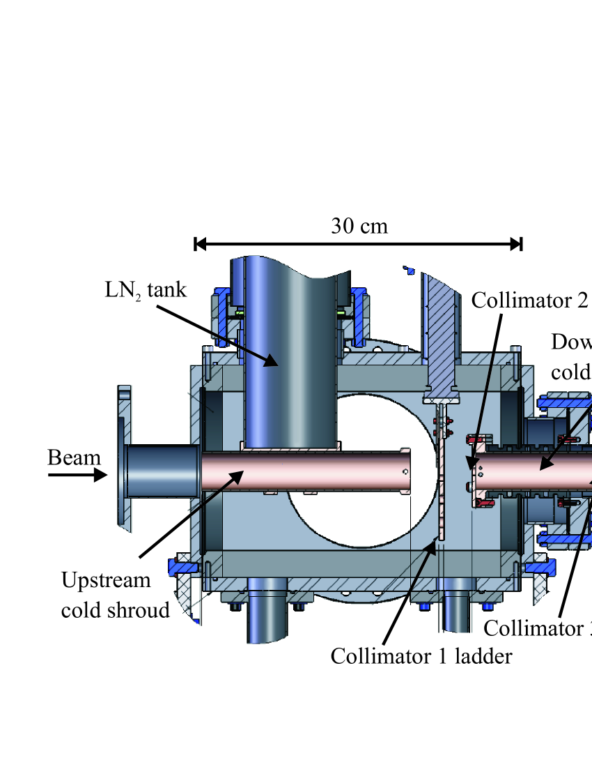
Figure 1: (color online) Side view of chamber cross section. Copper braids connecting the upstream and downstream cold shrouds have been omitted for clarity.

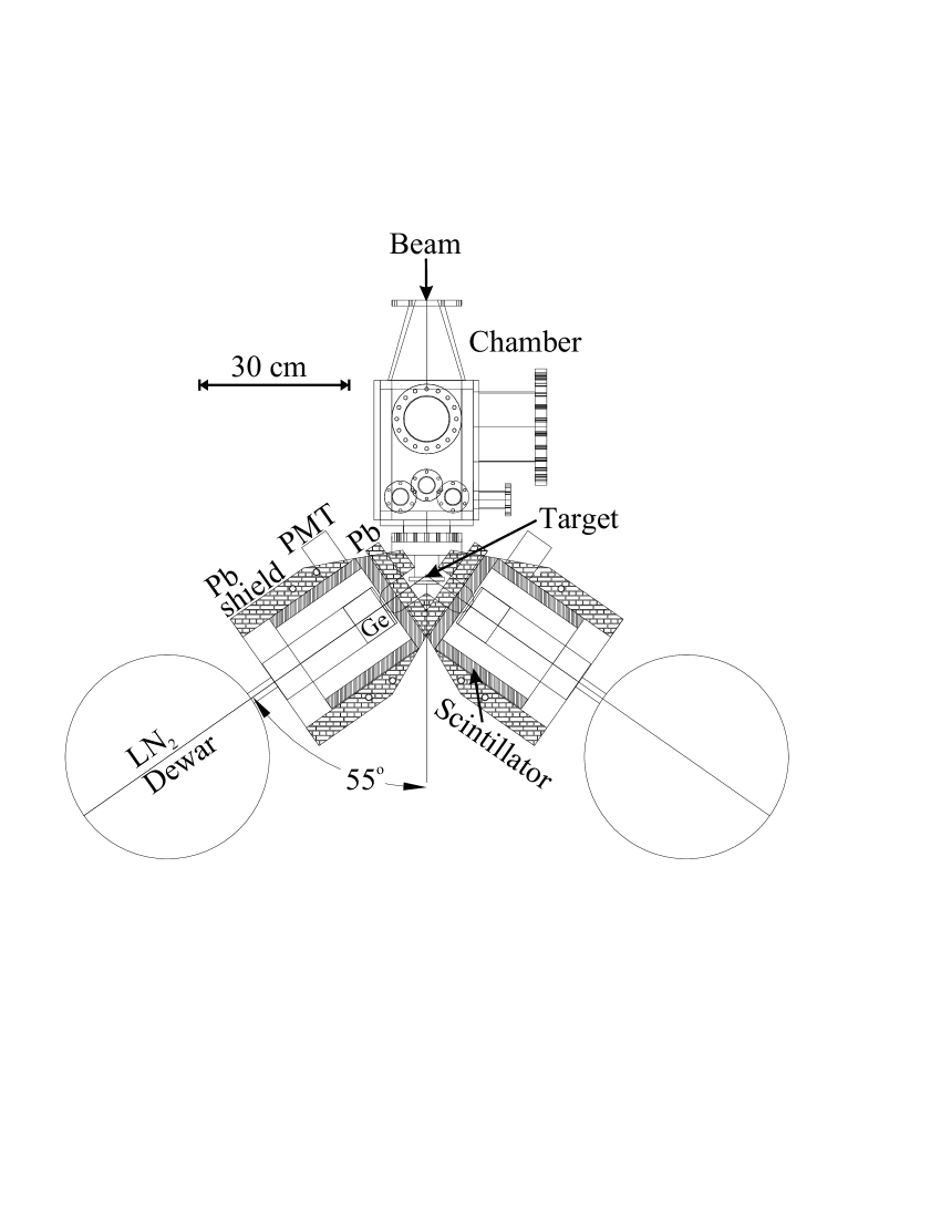
Figure 2: Top view of detector setup. The PMT shown is for the annular scintillator only; the planar scintillator PMT has been omitted for clarity.

Figs. 1 and 2 illustrate our chamber and detector system, respectively. The main features of the chamber included its dual liquid-nitrogen cooled cold shroud system, three collimators, and water-cooled target mount. The cold shroud isolated the radioactive target to prevent the contamination of the upstream beamline with ²²Na and also helped maintain a clean environment near the target, suppressing carbon buildup. During data collection, the pressure in the chamber was in the range of (1-2)$\times 10^{-7}$ torr. The end of the downstream cold shroud surrounded our target substrate; however, because it was the farthest away from the liquid-nitrogen cold trap, it only reached a temperature of 125 K, whereas the upstream shroud reached 88 K.

The chamber had three sets of collimators. The first, collimator 1, was a water-cooled, sliding ladder between the cold shrouds with 4-, 7-, and 8-mm diameter collimators. The 8-mm collimator was used during ²²Na($p,\gamma$) data acquisition. Also on this ladder were electron-suppressed 1-mm and 3-mm diameter collimators with downstream beam stops for tuning. Collimator 2, an 8-mm collimator, was 33 mm downstream of the ladder and was attached to the end of the downstream cold shroud. It was followed by a 10-mm diameter cleanup collimator, collimator 3, located 122 mm farther downstream. Each collimator was electrically isolated from the chamber to permit current monitoring.

The target substrate was bolted to a copper backing flange and was directly cooled with deionized-water via a thin pipe coupled to the flange. To minimize handling time in proximity to the radioactive targets, this assembly was then attached to a stainless steel coupler with a ISO flange on the chamber side. Directly upstream of this assembly was a 30-mm long electron suppressor biased between $-150$ and $-300$ V. During data collection, the current on target was monitored, and the charge was integrated and recorded.

Two sets of detector systems were positioned at $\pm$ 55^∘ to the beam axis. A top view of the setup, including chamber, shielding, detectors, and Dewars, is shown in Fig. 2. Each system consisted of a high-purity 100% germanium (HPGe) crystal Canberra model GR10024 encased in cosmic-ray anticoincidence shielding. The detector angle was chosen to minimize effects due to angular anisotropy, as the Legendre polynomial $P_{2}(\cos\theta)$ is zero at $\pm$ 55^∘. The resolutions for each detector at 1.275 MeV were 4.4 keV and 7.4 keV (FWHM) with high rates (²²Na target present), and 2.2 keV and 3.0 keV (FWHM) with low rates (using residual ²²Na activity with ²²Na target removed).

In addition, because of the target radioactivity, 26 mm of lead shielding was placed between the target and detector system to reduce the event rate in the detectors to a few tens of kHz. According to simulations, described in detail in Sec. II.5.1, the lead reduced the counting rate for the 511-keV gamma ray by a factor of 70, whereas the photopeak from 1275-keV gamma rays was reduced by a factor of 5. The suppression ranged from factors of $\sim$ 3.5 to 4.5 for gamma rays with energies above $\sim$ 5 MeV. Above 4 MeV, cosmic rays caused a continuum background. In order to remove these unwanted signals, 25-mm thick annular and planar plastic scintillators encased in lead, as shown in Fig. 2, were used in anticoincidence with the germanium detectors and are discussed in detail in the next section. The reduction of the ²²Na($p,\gamma$) signal by this veto was negligible.

II.4 Data Acquisition

In addition to the signals from the high-purity Ge detectors, the electronics also processed PMT signals from the scintillators. In order to reduce the rate seen by the detectors due to target radioactivity, two techniques were used: 1) lead shielding was installed as described above, and 2) a high threshold was set (just below the strong 1275-keV ²²Na line, so that the target activity could be monitored in-situ).

The Ge-signal amplifiers (ORTEC 672) were operated in a pile-up-rejection mode (which typically rejected $\sim$ 40% and introduced a dead time of 27 $\mu$s per pulse). Signals from the two sets of detectors were converted into digital signals by ORTEC AD413A ADCs with fast FERAbus readout, which helped to reduce dead time. A buffer module was used to minimize the communication with the computer via a CAMAC interface. JAM, a JAVA-based data acquisition and analysis package for nuclear physics Swartz et al. (2001), was used to process the data. All the NIM and CAMAC electronics modules were located in a temperature-controlled rack to minimize instabilities. The raw rate in each detector was below 30 kHz, and the trigger rate was $\sim$ 4 kHz. A sample background spectrum from one Ge detector is shown in Fig. 3.

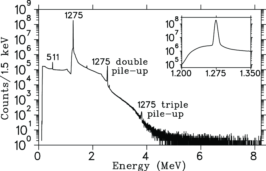
Figure 3: Sample background spectrum from one Ge detector, measured for $\sim$ 160 hours. Inset shows the spectrum expanded around the 1275-keV gamma ray.

Signals from the active anticoincidence shields and from the Ge detectors were used as a stop and start, respectively, in a Time-to-Amplitude-Converter (TAC). If these two signals occurred within a set timing window, the resulting Ge signal was discarded.

In order to determine the bounds of the TAC spectrum for data processing, the TAC signal corresponding to germanium detection energies between 4 and 6 MeV was extracted. The timing gate was set on the prompt peak, which had a long tail to its left. In this energy region, this anticoincidence system rejected $\sim$ 80% of the cosmic-ray background signal. The TAC signal for most high-energy cosmic rays from $\sim$ 6 to 11 MeV also falls within the set window. The scintillator threshold was set well above 511 keV to avoid vetoes by annihilation radiation. Self veto is possible with cascade gamma decays if one gamma ray is registered in the Ge and the other in the anticoincidence shield; this was examined by comparing the yields from raw singles spectra with those from the vetoed spectra, which agreed to better than 99%.

II.5 Detector Efficiency

Detector photopeak efficiencies were obtained by combining Penelope pen ; Salvat et al. (1997) simulations with direct measurements of gamma rays from ⁶⁰Co and ²⁴Na sources and from ${}^{27}{\rm Al}(p,\gamma)$ resonance measurements.

The efficiency at 1332 keV was determined using a 31.51-nCi ⁶⁰Co source. Isotope Products iso produced the source and measured its decay intensity with an uncertainty of 1.7% (99% $C.L.$). The geometry for the Penelope simulations was adjusted slightly to match the efficiency at this energy, as described in the following subsection. The ratio of efficiencies from 1369 to 2754 keV was measured using a ²⁴Na source ($t_{1/2}=15$ hrs) fabricated at the University of Washington. Since 1369 is very close to 1332 keV, we equated the efficiency at 1369 keV to the Penelope value, and then from this ratio we obtained the efficiency at 2754 keV.

To extend the efficiency determination to higher energies, we measured the ²⁷Al($p,\gamma$) reaction using a thick aluminum target and used the relative intensities of well-known gamma-ray branches from $E_{p}$ = 633 and 992 Endt et al. (1990); Meyer et al. (1975). For the latter resonance, our coin target was also used. We subtracted the below-resonance yield from the above-resonance yield to extract the net yield. At $E_{p}=992$ keV, the gamma rays of interest are at 1779, 4742, and 10762 keV. Using the simulation to determine the efficiency at 1779 keV, our measurements, combined with the known branches, gave the efficiencies at the two higher energies. At $E_{p}$ = 633 keV we measured the gamma rays at 7575 keV and 10451 keV. As the simulation matched the value we had obtained at 10762 keV, we used the simulation for the 10451 keV value and the known branch to determine the efficiency at 7575 keV. The agreement between measurement and simulation is discussed in the following subsection.

II.5.1 Penelope  Simulations

The geometry of our apparatus was modeled in the detailed Monte Carlo code Penelope. The simulated germanium detector included the germanium crystal, cold finger, and carbon window, with all dimensions taken from the nominal specifications provided by Canberra Canberra (2004). In addition, we included the 26-mm lead and 25-mm planar plastic scintillator in front of the detector. Although the annular plastic scintillator was modeled, the annular lead was not, as it was not in the line of sight of the target. The sodium source was a uniform 5-mm diameter disk centered on the copper substrate. The copper backing mount was included, as was the aluminum plate supporting the water cooling system. The water and its copper pipes inside the target mount were modeled, but the pipes that extended up and out from the mount were not, as they were thin and mostly out of the line of sight. All components of the target mount were aligned with the beam, whereas the detector was at an angle of 55^∘.

The gamma rays were projected from their source uniformly in a 80^∘ opening angle, which covered all modeled components, and absolute efficiencies were corrected for the solid angle. Each simulated energy included an initial number of gamma rays such that the photopeak precision was less than 0.1%. At $E_{\gamma}$ =1332 keV, with the source spread out over an area equal to that of the 1-mm diameter ⁶⁰Co source, the simulation initially gave results 2.5% higher than the measurement. Therefore, the front face of the crystal was moved back from the target by 1.7 mm, in order to make the simulation reproduce the measurement exactly. Results for the detector photopeak efficiency are shown in the upper panel of Fig. 4. The bottom panel of Fig. 4 shows the ratio of the measured efficiencies to the simulations. For sources other than ²²Na, source distribution and substrate material were changed in the simulation to match those used in the measurement.

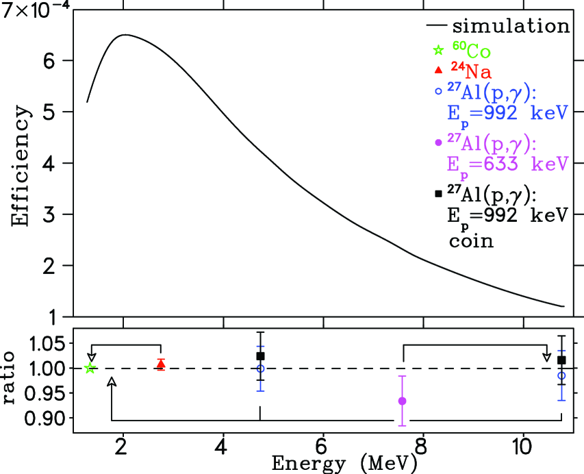
Figure 4: (color online) Photopeak efficiency. Top panel is the efficiency from Monte Carlo Penelope simulations. Bottom panel shows the ratio of efficiencies from measurement to simulation, and arrows indicate the gamma-ray energy used in the relative efficiency analysis.

For the 213- and 610-keV resonances in ²²Na($p,\gamma$), yields from first-escape peaks were added to the photopeak yield in order to improve statistics for branches with $E_{\gamma}$ = 7333 and 8162 keV, respectively. Comparison of ²⁷Al($p,\gamma$) data to simulation at 7.5 MeV indicates agreement to within 2% and is covered by the systematic error detailed in the next section.

II.5.2 Systematic Errors for the Efficiency

In order to extract systematic errors for our efficiencies, we compared the quality of the fit of our data from the ²⁴Na source and the 992- and 633-keV resonances of ²⁷Al($p,\gamma$) to our simulations, as shown in Fig. 4. The precisely measured ratio for the two ²⁴Na gamma rays yields a value for the efficiency at 2754 keV which is in agreement with that given by simulation. The points obtained from ²⁷Al($p,\gamma$) resonances have statistical uncertainties between 4.7 and 5.2%, and they agree well with the simulation. Therefore we ascribe a 5% systematic uncertainty to the efficiency determination for isotropic emission of gamma rays.

Because the detectors are centered at $\pm$ 55^∘ in the laboratory, zeros of $P_{2}(\cos\theta)$, the effect of a $P_{2}(\cos\theta)$ term in the angular distribution can only arise from the angular dependence of the efficiency across the detector and from center of mass to laboratory transformation. A $P_{4}(\cos\theta)$ term has no such restriction. Assuming the angular distribution to be of the form $\Omega(\theta)=1+a_{2}P_{2}(\cos\theta)+a_{4}P_{4}(\cos\theta)$, we used the Penelope  simulation to determine the effect of non-zero values of $a_{2}$ and $a_{4}$. A value of $a_{2}$ as large as 1 only caused a 2.6 $\pm$ 0.4% change in the efficiency. Published data for ²³Na$(p,\gamma)$ resonances Glaudemans and Endt (1963) show typical $a_{4}$ values of about 0.005 and a maximum value of 0.05. This maximum value would cause a 2.0 $\pm$ 0.4 % change in the efficiency. Therefore, we assigned an additional systematic error of 3%, to include the possible effects of the angular distribution. Our overall systematic error in the efficiency is $\pm$ 6%.

II.6 Beam Properties

II.6.1 Rastering

The beam was rastered using a magnetic steerer located 1 m upstream of the target. A rectangular pattern with 19- and 43-Hz horizontal and vertical frequencies was used, and signals proportional to the magnetic field were produced by integrating the voltage signals from a pickup coil located in the raster magnet. These readout values represent the center of the beam spot. For each data set collected, a 2-dimensional histogram of this signal in both horizontal and vertical directions was recorded. It was also possible to set a gate on the energy spectrum of each detector and sort out the corresponding raster fields.

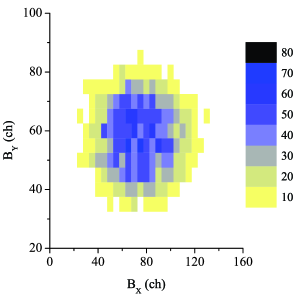
Figure 5: (color online) 2-dimensional raster plot on the “coin” target: a 5-mm diameter ²⁷Al disc embedded in copper. B_X and B_Y are proportional to the magnetic field of the raster. Shown is a histogram of the raster signal during a measurement of the 406-keV ²⁷Al($p,\gamma$) resonance, with a wide gate ranging from above the 7358-keV gamma ray to below its first-escape peak.

Fig. 5 shows this two-dimensional raster plot, obtained with a 5-mm diameter, 1.5-mm thick ²⁷Al disc embedded in the center of a copper backing. This “coin” target had the same OFHC copper substrate and diameter as our ²²Na targets. Shown are the counts detected for each value of the rastering field in the two dimensions. During all data-taking, the raster signals were monitored in order to diagnose problems with the target or other issues that may have arisen. For each measured resonance, the amplitude for the raster was scaled as the square root of the proton energy, so the rastered area of the beam on target would be constant.

II.6.2 Energy and Density

The beam energy was determined using a 90^∘ analyzing magnet with an NMR field monitor and calibrated using resonances in ²⁷Al($p,\gamma$) at $E_{p}$ = 326.6, 405.5, 504.9, and 506.4 keV. Given the quality of the fit, we assign a $\pm$ 0.5 keV uncertainty to our knowledge of the beam energy.

We also conducted measurements on ²⁷Al targets in order to extract the normalized beam density, averaged over the 5-mm diameter area. Systematic errors were then explored with simulation and visual inspection of beam-related target coloration. Beam non-uniformity was then taken into account, and its effect combined with the possibility of a non-uniform target was investigated.

We determined the normalized beam density, $\rho_{b}$, averaged over the target, by comparing the thick–target yield from our “coin” target, $Y_{c}$, which had the same areal extent as the ²²Na targets, to the yield from a solid ²⁷Al target, $Y_{s}$. From the ratio of these yields, one can extract $\rho_{b}$ via:

$$\frac{Y_{c}}{Y_{s}}=\rho_{b}A_{c},$$ (5)

where $A_{c}$ is the area of the coin. The yields were measured at different times with different beam tunes using the resonances at $E_{p}$ = 406 and 992 keV, which yielded results for $\rho_{b}$ of $2.60\pm 0.09{\rm~{}cm}^{-2}$ and $2.55\pm 0.10$ cm^-2, respectively, with statistical errors only. The weighted average of these two measurements, 2.58 cm^-2, was chosen for $\rho_{b}$.

To study the distribution of beam across the target in order to quantify systematic errors, we carried out a number of measurements using a large raster with $1.8\times$ the standard amplitude, in addition to the standard amplitude, on the main ²²Na targets and the solid ²⁷Al and coin targets. With the raster on and off, transmission measurements through various collimators, shown in Fig. 1, were performed as well. These measurements, along with the relative yields of large to standard raster, were used to constrain a Monte Carlo simulation, described below, that was used to investigate potential beam densities on the target. It also was used to test the effects of possible beam drift, misalignment of the beam and target, and target non-uniformities.

The simulation modeled transport of the beam through the final components of the beamline and chamber, including the final quadrupole, the rastering unit, and the three sets of collimators. Variable parameters included beam width and offset, possible collimator offset, raster amplitude, and beam distribution at the quadrupole. A normalized beam density could not be uniquely determined by this method alone, but the densities within an acceptable phase space, defined by reasonable agreement for transmissions and large/standard rastering yield ratios, ranged from 2.33 to 2.83 cm^-2. Even for the extreme case where the quadrupole aperture is filled uniformly, the beam density was found to vary by less than 15%. We adopted $\pm$ 0.25 cm^-2 as the systematic uncertainty in the normalized beam density.

III Data and Analysis

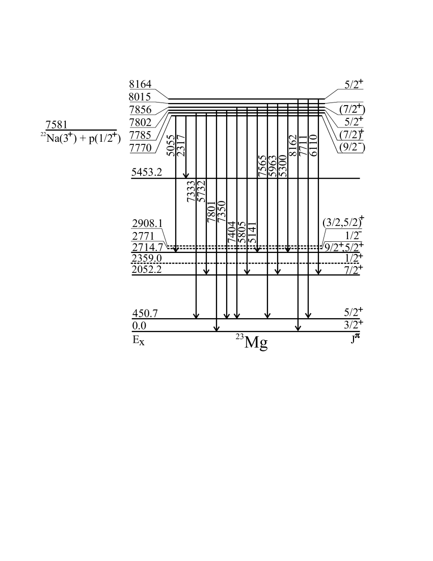
Figure 6: The relevant part of the decay scheme of ²³Mg. Energies are in keV. Not all ²³Mg levels are shown.

Measurements were taken on previously known ²²Na($p,\gamma$) resonances, which we find at $E_{p}=$ 213, 288, 454, and 610 keV. We also explored the proposed resonances at 198, 209, and 232 keV. The relevant energy level diagram for ²³Mg is shown in Fig. 6.

For all measurements, an energy scan was performed across a $\sim$ 25 keV range about the nominal resonance energy. To subtract background, which was comprised mostly of cosmic rays and Compton events, we assumed it to have a localized linear dependence on gamma-ray energy and fit the background to windows in the spectrum above and below the line of interest. This method was especially important for resonances with characteristic gamma rays below 6 MeV. Here contributions from 6129-keV incident photons due to the contaminating ¹⁹F($p,\alpha\gamma)^{16}$O reaction were significant. Affected resonances included $E_{p}$ = 454, 288 keV, and one branch from $E_{p}$ = 610 keV.

In order to extract the yield at each laboratory proton energy, $E_{p}$, an energy window was set on the gamma ray of interest in the vetoed singles spectrum for each of the two germanium detectors. This window was $\sim$ 25 keV for one detector and $\sim$ 40 keV for the other. For each detector, the sum of the background subtracted counts in the window is $N_{i}=N_{\rm prod}\eta_{i}L_{i}$, where $\eta_{i}$ is the efficiency, and $L_{i}$ is the live time for detector $i$. Then the yield is

$$Y=\frac{N_{\rm prod}}{Q/e}=\frac{{N_{1}}/{L_{1}}+{N_{2}}/{L_{2}}}{\eta Q/e},$$ (6)

where $\eta=\eta_{1}+\eta_{2}$. The effects of angular distributions have been addressed in Sec. II.5.2. In order to determine the live time, a signal from a pulser unit was fed into the “test” port of each Ge preamplifier, creating an additional signal in the corresponding amplitude spectra. This signal was sorted into its own spectrum by a logic signal to the data acquisition. A window of comparable width to the energy window for the yield was placed on the prompt pulser signal and compared to the scaled number of pulser pulses. This ratio gave the live time, which ranged from 35 to 45% for the radioactive targets and was above $\sim$ 90% for all other targets. The live-time correction was substantial, but it was not beam-related; instead it resulted from a constant rate due to the radioactivity. To test the accuracy of the live-time correction, a thick ²⁷Al target was irradiated with protons with and without a ²²Na source nearby. Although the presence of the radioactivity decreased the live time from 97% to 50%, the ratio of the live-time corrected yields was 0.99 $\pm$ 0.02.

In order to test the sensitivity of our results to the inputs for the gamma-ray background subtraction and its linearity, resonances at $E_{p}=610$ keV (with $E_{\gamma}=8162$ keV) and 454 keV (with $E_{\gamma}=5300$ keV) were inspected, and the choice of window for both the peak and the background on each side was varied to reasonable limits, such as widening, shortening (no window smaller than 10 keV), and shifting. The resonance strengths changed by less than 1%, indicating that systematic errors associated with background subtraction are negligible.

After the yields for each excitation function were determined, the areas under the excitation curve were estimated by using the trapezoidal method. This value for $\int Y_{i}\,dE$ was then used in Eq. 4, along with values determined for all other parameters, to extract the partial resonance strength, $\omega\gamma_{i}$, for each branch $i$. The total strength is simply equal to the sum of the partial strengths for all branches.

III.1 Yields

III.1.1 Absolute Yields: $E_{p}$ = 610, 454, 288, 213 keV

Fig. 7 shows the data taken on the two strongest resonances at $E_{p}=454$ and 610 keV. These resonances were revisited after various amounts of accumulated charge to monitor possible target degradation, discussed in detail in Sec. III.2. Fig. 8 shows the corresponding gamma-ray spectra summed over all runs, including an inset illustrating the background subtraction method. All data for resonances at $E_{p}$ = 213, 288, and 610 keV were taken on target #4, and the 454-keV resonance was measured on both targets #3 and #4.

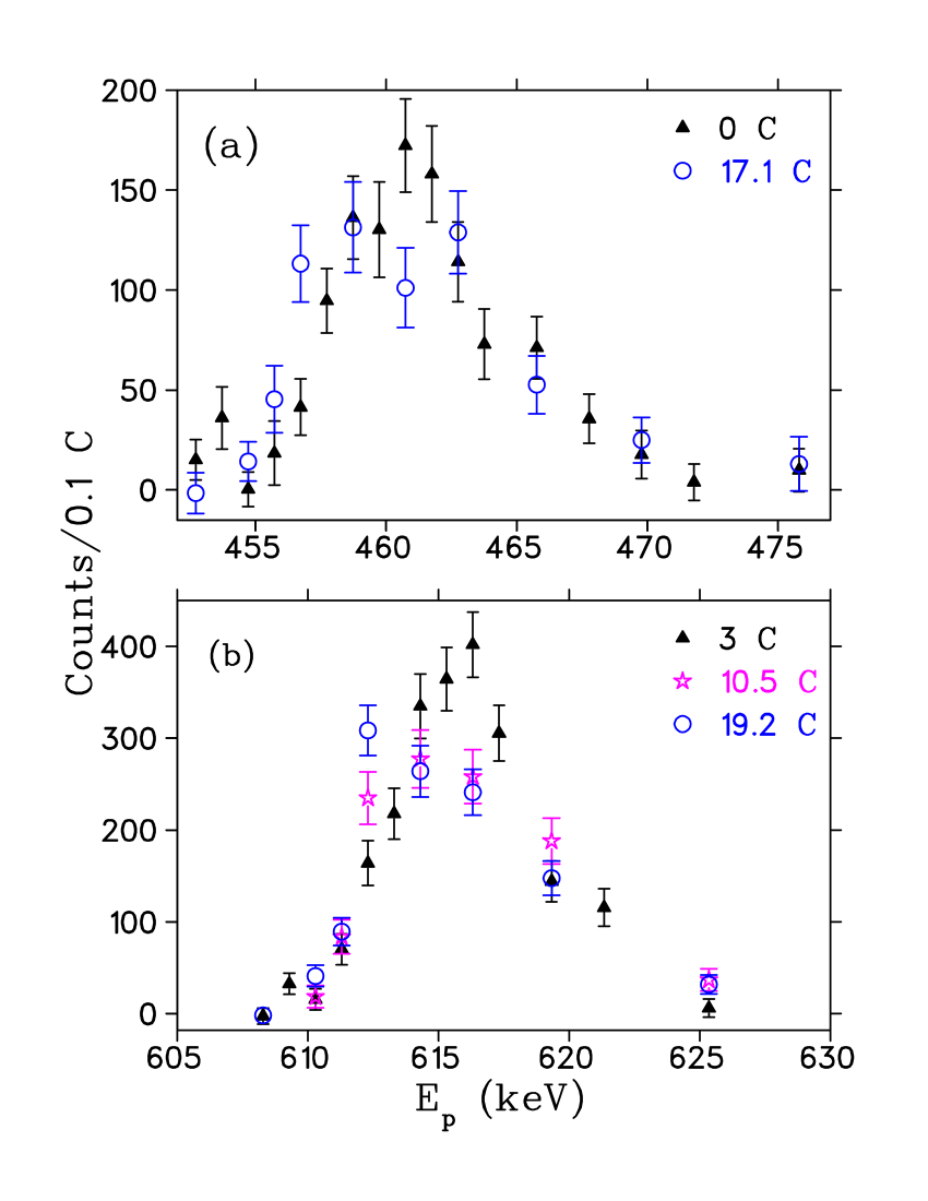
Figure 7: Excitation functions for (a) $E_{p}$ = 454 keV and (b) $E_{p}$ = 610 keV. $E_{p}$ is the lab proton energy. Each plot shows the excitation function at the beginning of target bombardment and at the end, after $\sim$ 20 C had been deposited. An intermediate curve after 10.5 C is also shown in (b). (a) is gated on E${}_{\gamma}=5300$ and 5963 keV, and (b) is gated on the photopeak and single-escape peak of E${}_{\gamma}=8162$ keV.

Figure 8: Summed gamma-ray spectra for (a) $E_{p}$ = 454 keV and (b) $E_{p}$ = 610 keV. The inset illustrates the beam-background subtraction method for E${}_{\gamma}=5300$ keV, including gamma-ray gate (dashed), analytically calculated background line (solid), and subtracted region (hatched). SE and DE indicate single- and double-escape peaks, respectively.

Fig. 9 illustrates the summed raster plots for target #3 with $E_{p}=454$ keV. The concentration of counts from ²²Na($p,\gamma$) are well centered, while a few counts spread through the plot are consistent with yield from ¹⁹F contamination.

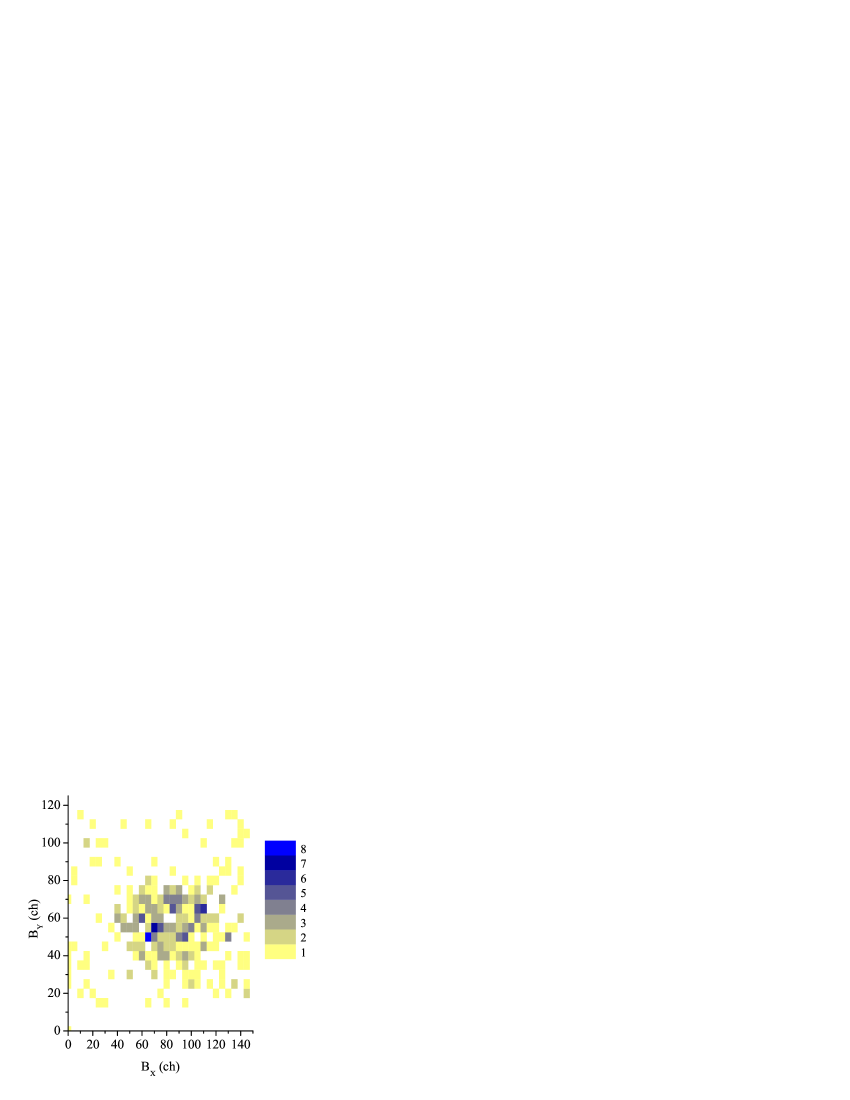
Figure 9: (color online) Raster plot for the sum of ²²Na($p,\gamma$) for $E_{p}$ = 454 keV, target #3, with raster amplitudes $1.8\times$ larger than our standard amplitudes. The plot is gated on $E_{\gamma}$ = 5300 keV. Outside the target area there are a few bins with only 1 count, which is consistent with the known level of ¹⁹F contamination from the Compton continuum from $E_{\gamma}$ = 6129 keV.

Fig. 10 shows the data taken for 288- and 213-keV resonances, and Fig. 11 illustrates the summed gamma-ray spectra for each resonance, respectively. Characteristic gamma rays for each are clearly distinguishable above background. For $E_{p}=213$ keV, the integrated yield was determined with the same trapezoidal method as other resonances, plus a small correction because the highest energy point did not reach zero yield. The details of determining this contribution are discussed in Sec. III.1.3, after a prerequisite analysis method is outlined in the following section.

Figure 10: Excitation functions for (a) $E_{p}$ = 288 keV and (b) $E_{p}$ = 213 keV. $E_{p}$ is the lab proton energy. (a) is gated on E${}_{\gamma}=5141$ keV, and (b) is gated on the photopeak and single-escape peak of E${}_{\gamma}=7333$ keV.

Figure 11: Summed gamma-ray spectra for (a) $E_{p}$ = 288 keV and (b) $E_{p}$ = 213 keV. SE and DE indicate single- and double-escape peaks, respectively.

III.1.2 Upper Limits for Yield: $E_{p}$ = 198, 232, 209 keV

Data in the region of the proposed resonances at $E_{p}=198$ and 232 keV are shown in Fig. 12. In the summed gamma-ray spectra shown in Fig. 13, no discernible gamma-ray yields can be detected above background. All data for $E_{p}$ = 198 keV were taken on the chromium-covered target #3. Data for $E_{p}$ = 232 keV were taken on one of the bare test targets, which had previously been exposed to an integrated charge of 13 C.

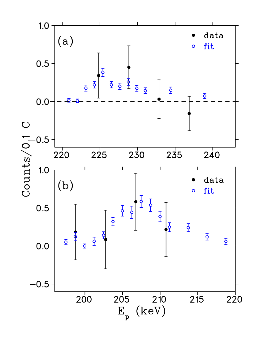
Figure 12: (color online) Solid circles are excitation functions for (a) $E_{p}$ = 232 keV and (b) $E_{p}$ = 198 keV. $E_{p}$ is the lab proton energy. (a) is gated on E${}_{\gamma}=5055$ keV, and (b) is gated on the sum of E${}_{\gamma}=7801$ and 7350 keV. Open circles are the normalized, stretched, and shifted $E_{p}=454$ keV excitation function fit, described in the text. This reference excitation function is not as smooth in (a) as in (b) due to degradation of the bare target.

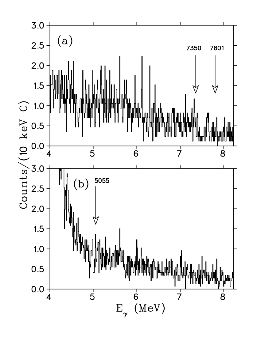
Figure 13: Summed gamma-ray spectra for (a) $E_{p}$ = 232 keV and (b) $E_{p}$ = 198 keV. The target activity was $2.3\times$ higher in (b) than in (a) and is responsible for the increased background at low energies. Arrows indicate the energy where one would expect to see gamma rays from the relevant transition.

For these resonances, the shape of the excitation function used to determine the area was adopted from either the resonance at $E_{p}$ = 454 or 610 keV, depending on the target. Because the resonance shape was dominated by the implantation distribution, this shape was normalized, shifted, and stretched so that it could be fit to the data of the resonance in question. The stretch factor was fixed and set equal to the ratio of stopping powers in copper for the two energies, whereas the energy shift and the normalization factor were allowed to vary. The central value of the shift was given by the differences in resonance energies, and the range of the shift was given to fully span the data points. If a data point for the low-energy resonance fell between points of the normalized curve, the corresponding reference point was determined by a linear interpolation. For each pair of shift and normalization, the value of the $\chi^{2}$ between each low-energy resonance and the normalized reference resonance was calculated. The modified reference excitation function corresponding to the minimum value of $\chi^{2}$ is shown for each resonance in Fig. 12 (open circles).

Figure 14: Projection of exp$(-\chi^{2}(\omega\gamma_{i},E_{i})/2)$ onto the $\omega\gamma$-axis for (a) $E_{p}$ = 232 keV and (b) $E_{p}$ = 198 keV. The curves represent the probability density functions, used in Sec. V.

The array of probabilities, $P(\omega\gamma_{i},E_{i})$, was taken to be proportional to exp$(-\chi^{2}(\omega\gamma_{i},E_{i})/2)$, where $\chi^{2}(\omega\gamma_{i},E_{i})$ is the $\chi^{2}$ between the model, assuming particular values for $\omega\gamma_{i}$ and $E_{i}$, and the data. Because we are mainly interested in constraining the value of $\omega\gamma$, we projected the two-dimensional arrays onto the $\omega\gamma$-axis (i.e. $P(\omega\gamma_{i})=\sum_{E_{i}}P(\omega\gamma_{i},E_{i})$), shown in Fig. 14. The upper limits on $\omega\gamma$ were extracted with a particular confidence level, $C.L.$, using the likelihoods:

$$C.L.=\frac{\displaystyle\sum_{\omega\gamma_{i}=0}^{\omega\gamma}P(\omega\gamma_{i})}{\displaystyle\sum_{\omega\gamma_{i}=0}^{\infty}P(\omega\gamma_{i})}.$$ (7)

The sum in the denominator was cut off at a maximum value of $\omega\gamma$ such that the sum changed by less than 1%. Results are given in Sec. IV.

For the possible resonance at 198 keV, a finite value for the strength was also calculated. Instead of summing from zero and extending upward in the numerator of Eq. 7, the pair of $\omega\gamma_{i}$ values with equal values of $P(\omega\gamma_{i}$) were determined such that the sum between them, properly normalized, gave the desired confidence level. Because of its small branch, data for the third possible gamma-ray for $E_{p}=232$ keV at $E_{\gamma}$ = 5749 keV was not added to our yield; however, branches from the two other gamma rays were used to adjust the total resonance strength.

For the proposed resonance at $E_{p}$ = 209 keV, we also applied this method to a hybrid data set comprised of measurements around the resonances at $E_{p}=198$ to 213 keV for the gamma ray at 5067 keV, assuming the branch given by Jenkins et al. Jenkins et al. (2004) and using the excitation function from the dominant branch of $E_{p}=213$ keV and its first-escape peak as the reference curve. Because the data from the resonance at 198 keV were from a different target, its yields were scaled by the ratio of measured target activities. The shift in energy was allowed to vary from zero to 25 keV, and the fit yielding the minimum $\chi^{2}$ was found at the position of the 198-keV data points, possibly due to the fact that the gamma rays have overlapping energy windows. In other words, we did not observe a separate resonance at $E_{p}$ = 209 keV. An upper limit for this resonance, which is presented in Sec. IV, was extracted by restricting the energy shift to be equal to the difference in resonance energies, spanning the range of $\pm~{}2\sigma$ around the value claimed by Jenkins $\it{et}$ $\it{al}$ Jenkins et al. (2004).

This analysis technique of normalizing and shifting a reference resonance to obtain strengths of others was validated by applying it to the 288-keV resonance, for which the ratio of the strength calculated from this method to the direct method was 0.95 $\pm$ 0.12.

III.1.3 Corrected Area for $E_{p}=213$ keV

In order to estimate the full area of the $E_{p}=213$ keV excitation function, a reference resonance measurement at $E_{p}=454$ and three at $610$ keV were utilized in the same manner outlined above. Each of the four curves were fit to the data, and each yielded a data point beyond the fixed $E_{p}=213$ keV excitation function that did reach zero. The last trapezoid area was calculated for each, and the average was added to the area from the direct data, equaling $10\pm 5$% of the total area. The uncertainty in the additional area was set to be the standard deviation among the four fits.

III.2 Total Number of Target Atoms

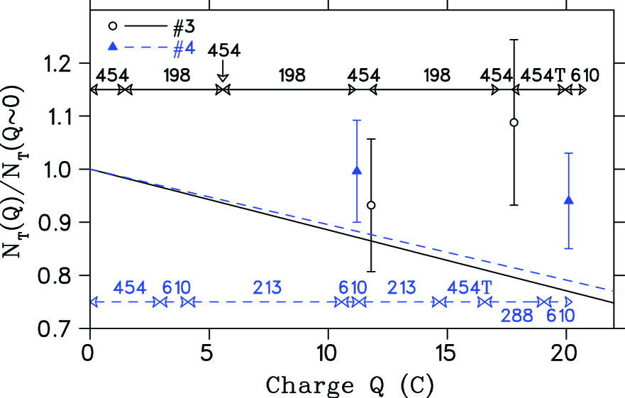
Figure 15: (color online) Target degradation as a function of accumulated charge for main targets #3 and #4. $N_{T}(Q)$ is the total number of atoms present in the substrate after an irradiation of charge, $Q$. The data points illustrate the ratio of the area of each reference excitation function to its initial area at the start of target bombardment. The lines represent a possible linear decrease of the number of atoms deduced from two residual activity measurements at the beginning and end of bombardment. Also shown is the timeline for each resonance measurement. The two sections marked “454T” indicate variable raster amplitude tests, and although these data are included in the branching ratio determination, they are not included in determining resonance strengths.

We determined the initial number of target atoms from the 1275-keV gamma rays emitted in the decay of ²²Na ($t_{1/2}$ = 2.6027(10) yrs nnd ) and assigned a 2.6% uncertainty. This uncertainty combines the 1.7% uncertainty in the ⁶⁰Co calibration source at $E_{\gamma}=1332$ keV with an additional 2% due to the accuracy of the $\sim$ 7% background subtraction in this region of high detector rate.

However, measuring the activity in-situ was not sufficient to determine the total number of target atoms throughout the measurement. During target bombardment, some fraction of ²²Na was sputtered out of the illuminated area of the substrate, yet it remained nearby, maintaining an approximately constant activity throughout the duration of the resonance measurements. Thus, in addition to determining the total number of initial atoms, monitoring possible target degradation throughout bombardment was particularly important.

In order to deduce the amount of degradation, two complementary methods were utilized. One method was to revisit a strong reference resonance periodically throughout the bombardment cycle. We define $A(Q)$ as the integral of the reference excitation function, $\int YdE$, after an amount of charge, $Q$ has been deposited. $A(Q)$ is directly proportional to the number of target atoms, $N_{T}(Q)$, as shown in Eq. 4. The ratio of the integrals of the excitation function before and after bombardment, $A(Q)/A(Q\sim 0)$, is therefore equal to $N_{T}(Q)/N_{T}(Q\sim 0)$. The second method, which will be described in detail later in this section, was to measure the residual ²²Na in the chamber before and after target bombardment and use this information to infer the number of sputtered target atoms. The results of each method are illustrated in Fig. 15, along with a timeline for each resonance measurement as a function of accumulated charge.

Target #3 accumulated 20.7 C in 186.0 hours, and target #4 accumulated 20.1 C of charge in 138.3 hours. Because we covered these targets with 20 nm of chromium, they remained fairly stable. Shown in Fig. 7 (a) are the first and last resonance scans at $E_{p}$ = 454 keV for target #3. Throughout the 20.7 C of bombardment, the resonance at $E_{p}$ = 454 keV was revisited four times. $A(Q\sim 20$ C$)/A(Q\sim 0)$, shown in Fig. 15, is 1.07 $\pm$ 0.12, consistent with no target loss. For target #4 on which all other non-zero strength resonances were measured, the monitoring resonance was $E_{p}$ = 610 keV, and multiple scans of its excitation function are shown in Fig. 7 (b). At the end of bombardment, $A(Q\sim 20$ C$)/A(C\sim 0)=0.94\pm$ 0.09, which is consistent with no target loss.

To use the residual activity method, measurements of the 1275-keV rate were taken before target installation ($R^{i}_{0}$), after target installation and before bombardment ($R^{i}_{T}$), after bombardment ($R^{f}_{T}$), and after target removal ($R^{f}_{0}$). The quantity $(R^{i}_{T}-R^{i}_{0})-(R^{f}_{T}-R^{f}_{0})$ then is proportional to the amount sputtered from the target. This final value was used to estimate target degradation throughout the bombardment, assuming linear loss, and is also shown in Fig. 15 for each target. As we learned with our ²³Na tests Brown et al. (2009), this loss is in fact not linear but usually begins to occur after a significant amount of charge has been deposited, removing the protective layer and sputtering away some of the substrate. We nevertheless used a hypothesis of linear degradation of the target for one extreme of $N_{T}$ and an amount consistent with no loss for the other.

The 198-, 213-, and 232-keV resonance measurements were taken over an extended period of time and charge, whereas all others were measured with a few Coulombs of integrated beam current and did not experience possible prolonged degradation. The 198- and 213-keV data were taken over $\sim$ 15 and 10 C, respectively, with short interruptions to measure the reference resonance excitation functions. At the halfway point for each, the linear-decrease hypothesis indicated a 4-5% loss, although excitation function areas are consistent with no loss at that point. Therefore, we choose no loss with errors that span the values from each method, $N_{T}(Q)/N_{T}(Q\sim 0)=1.00^{+0.00}_{-0.05}$. Combining this with the systematic uncertainty in the initial number of atoms, we have an overall systematic error of $+2.6$% and $-5.6$% in the total number of atoms for the 198- and 213-keV resonance strengths. For the 454- and 610-keV resonances, which were each measured at the beginning of target bombardment, only an overall systematic error of $\pm 2.6$% was needed.

The 288-keV resonance was a special case, as its data were not from an extended measurement but were taken after 18 C of irradiation. Directly following the measurement of this resonance, we performed the final scan of the 610-keV reference resonance, which allowed insight into how many atoms remained. Therefore, the total number of atoms present for the 288-keV measurement was taken to be the average between linear target loss and loss indicated from the depleted area of the 610-keV resonance curve, $N_{T}(Q)/N_{T}(Q\sim 0)=0.88^{+0.12}_{-0.06}$. Because target loss is not actually linear and could have happened after the 288-keV resonance measurement, the uncertainties span the range between no loss and the value given by linear loss.

The 232-keV resonance data were taken with a test target with no protective layer after 13 C had already been bombarded, and target loss was appreciable. At the end of the $\sim$ 20 C irradiation, measurements of the residual activity indicated a 68% loss. As explained above, loss is not linear and occurs quite rapidly at the end of the cycle. Because of this fact, we have chosen to take the loss only from the difference in monitoring the resonance areas, which were taken directly before and after the measurement and gave $A(Q)/A(Q\sim 0)=0.59$. This value was used to adjust the upper limit on the strength, and we assigned a systematic uncertainty of $\pm$ 40% to span a wide range approximately down to the value of linear loss. Regardless, the upper limit on this resonance strength is still dominated by the statistical uncertainty.

III.3 Systematic Error Summary

The systematic error budget for resonance strengths is shown in Table 1. In summary, we find an overall systematic error of $-11.7$% and $+12.7$% for the extended measurements at $E_{p}=198$ and $213$ keV, resulting from combining uncertainties of $\pm 6$% in the efficiency, $\pm 10$% in the normalized beam density, and $-2.6$% and $+5.6$% from the number of target atoms. For the resonances at $E_{p}=454$ and $610$ keV, the overall systematic uncertainty is $\pm 11.7\%$, and for the resonance at $E_{p}=288$ keV it is $-18.1$% and $+13.4$%, differences all due to the differing number of target atoms. The 232-keV resonance has the largest overall uncertainty, $\pm 42\%$.

Table 1: Summary of systematic errors for each resonance strength. Note, the total error for the resonances at $E_{p}=198$ and 232 keV is dominated by statistical errors.

	$E_{p}$ (keV)
Systematic Error	454/610	213/198	288	232
Efficiency	6%	6%	6%	6%
Normalized beam density	10%	10%	10%	10%
Total number of atoms	$2.6$%	${}^{+5.6}_{-2.6}$%	${}^{+7}_{-14}$%	$40$%
Total	11.7%	${}^{+12.7}_{-11.7}$%	${}^{+13.4}_{-18.1}$%	42%

III.4 Resonance Energies

We were able to obtain resonance energies with two separate techniques. First, we extracted the resonance energy from the observed gamma-ray energy, along with the excitation energy of the daughter level nnd and Q-value (7580.53 $\pm$ 0.79 keV, using the newly measured masses of ²³Mg Saastamoinen et al. (2009) and ²²Na Mukherjee et al. (2008)). From a thick-target ²⁷Al($p,\gamma)$ measurement at $E_{p}$ = 406 keV, the spectrum was calibrated using transitions energies 5088.05 and 7357.84 keV and each first-escape peak from the corresponding gamma rays. Energies were corrected for Doppler shift and recoil, which ranged in magnitude from $\sim$ 4 to 7 keV and $\sim$ 0.6 to 1.5 keV, respectively. Because the detector gain depended slightly on rate, a correction ranging in magnitude from 2.4 $\pm$ 0.7 to 3.8 $\pm$ 1.1 keV was also applied. This was determined by measuring the shift in the calibration gamma-ray energies with and without ²²Na sources nearby.

Second, we found the resonance energy from the proton energy, via the excitation function. The energy at which the yield reached half its maximum was determined, and the losses in the 20-nm chromium layer and 4 nm of copper were subtracted. This copper depth is the depth at which the ²²Na distribution reached half of its maximum value. According to simulations using TRIM tri , the total subtracted losses were $\sim$ 3 to 5 keV, and a 20% uncertainty in the stopping power was assumed. For the 213- and 288-keV resonances, an additional adjustment to the resonance energy was added to account for the slight transformation of the excitation functions due to sputtering, as shown in Fig. 7 (b). From repeated scans of the 610-keV resonance, the energy at half of the maximum yield changed by 1.2 $\pm$ 0.9 keV after 11 C, in the middle of the 213-keV resonance measurement, and that shift remained constant after 19 C, directly after the 288-keV measurement. Those resonance energies were adjusted by that amount. Results are given in Sec. IV. Similarly, excitation energies, $E_{x}$, and gamma-ray energies, $E_{\gamma}$, each were found independently by using the weighted average of the respective value extracted from the excitation function and the respective value extracted from the gamma-ray spectra.

III.5 Branches

Strong branches were determined from the spectra summed over all runs within a particular resonance. For resonances at $E_{p}=454$ and 610 keV, which were used as reference resonances to monitor degradation and for other target tests, the total amount of data was significantly larger than for a single resonance scan.

Due to the very low statistics for weaker possible branches, an additional restriction was placed on the analysis. Similar to our analysis for weak resonances where a reference resonance excitation function was shifted and normalized to fit the data, the excitation function for the strongest branch (and its first-escape peak for branches from $E_{p}=610$ keV) was normalized to match the weaker branches’ excitation functions, such that the $\chi^{2}$ was minimized. Then the branches were extracted using Eq. 7.

Only an upper limit for the branch at $E_{\gamma}=6112$ keV from the $E_{p}=610$ keV resonance could be obtained due to the obscuring peak at $E_{\gamma}=6129$ keV from ¹⁹F contamination. In order to estimate the contribution from the ²²Na($p,\gamma$) resonance, the spectral line shape was deconvolved into the contribution from ¹⁹F and from ²²Na. This was done by comparing the on-resonance line shape with the sum of the off-resonance line shape and a shape representing the 6112-keV gamma ray. The latter shape was estimated from a normalized and shifted peak at $E_{\gamma}=8162$ keV, the largest branch in the de-excitation. The value of this normalization was equal to the ratio of the magnitude of the branches, adjusted for efficiency differences, and was extracted by minimizing the $\chi^{2}$ of the hybrid curve and the on-resonance curve. Because of the changing shape of the off-resonance curve above and below the resonance, only an upper limit could be obtained.

III.6 Verification of Experimental Method

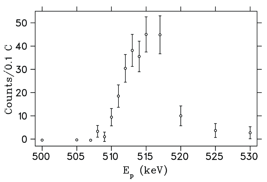
Figure 16: Excitation function for ²³Na($p,\gamma$) resonance at $E_{p}$ = 512 keV gated on $E_{\gamma}=10810$ keV. $E_{p}$ is the lab proton energy.

In order to verify our technique, targets of ²³Na were implanted using the ion source on the injector deck at the low-energy end of the University of Washington accelerator, and known ²³Na($p,\gamma$) resonances were measured under the same conditions as the ²²Na($p,\gamma$) measurements. A 20-nm layer of chromium was also evaporated on the surface, similar to the main ²²Na targets.

The ²³Na($p,\gamma$) resonance at $E_{p}$ = 512 keV has a reported strength of 91.3 $\pm$ 12.5 meV and is the recommended reference resonance for this reaction Iliadis et al. (2001). We measured this with a target containing (5.8 $\pm$ 0.9) $\times 10^{15}$ atoms, as determined by implantation charge integration with a measured correction for the sputtering of positive ions. The excitation function is shown in Fig. 16. Using the 10810-keV gamma ray with a branch of 71% Meyer et al. (1972), we determined its total resonance strength to be 79 $\pm$ 17 meV, after applying the correction described below.

Inspection of the raster plot indicated a small part of the target was missed when using our standard raster. To determine the missing fraction, the target was illuminated with a larger raster amplitude that fully encompassed the target atoms. Comparing the full target area to the fractional area covered with the standard raster, the amount missed was estimated to be $\sim$ 12%. This correction was applied to the resonance strength. This was not necessary with our ²²Na targets, as their respective raster plots indicated the beam covered the entire active area. To estimate a range for the effect of the observed ²³Na target misalignment, simulations were performed, as described in Sec. II.6.2, with an offset of 1.5 to 2.0 mm and a variety of target distributions. The uncertainties associated with these calculations dominate the overall uncertainty quoted above.

IV Results and Discussion

Table 2: Resonance energies. Values are extracted from the lab proton energy, $E_{p}$, via the excitation function, correcting for energy loss $E_{\rm loss}$, and from the gamma-ray energy, $E_{\gamma}$. Statistical uncertainties are given for each individual branch, and combined branches include systematic uncertainties. The adopted value is the weighted average of both methods. All values are in keV.

Previous	Present
			$E_{p}$ (from excitation function):		$E_{p}$ (from $E_{\gamma}$):
$E_{p}$	Eγ	$E_{\rm loss}$	branch	combined branches	branch	combined branches	Adopted $E_{p}$
213.3 $\pm$ 2.7	7332.7 $\pm$ 1.2	5.1 $\pm$ 1.0	213.1 $\pm$ 3.0	213.1 $\pm$ 3.4	213.6 $\pm$ 1.6	213.6 $\pm$ 1.6	213.5 $\pm$ 1.4
287.9 $\pm$ 2.1	5140.6 $\pm$ 1.0	4.6 $\pm$ 0.9	286.5 $\pm$ 2.1	286.3 $\pm$ 2.3	288.4 $\pm$ 1.7	288.7 $\pm$ 1.3	288.1 $\pm$ 1.1
	5803.2 $\pm$ 1.3		285.6 $\pm$ 4.2		289.1 $\pm$ 2.0
457 $\pm$ 2	5300.1 $\pm$ 0.8	3.7 $\pm$ 0.8	452.8 $\pm$ 0.8	452.8 $\pm$ 1.1	455.6 $\pm$ 1.7	455.7 $\pm$ 1.1	454.2 $\pm$ 0.8
	5962.7 $\pm$ 0.8		452.8 $\pm$ 1.1		455.9 $\pm$ 1.6
611.3 $\pm$ 1.8	8162.3 $\pm$ 0.9	3.2 $\pm$ 0.7	609.6 $\pm$ 0.9	609.0 $\pm$ 1.1	611.0 $\pm$ 1.5	610.8 $\pm$ 1.2	609.8 $\pm$ 0.8
	7711.2 $\pm$ 1.1		608.1 $\pm$ 1.1		610.3 $\pm$ 2.0

Results are shown in Tables 2, 3, and 4. The resonance energies are summarized in Table 2, the gamma-ray branches and partial strengths for each resonance are summarized in Table 3, and the final resonance strengths are summarized in Table 4.

The resonance energies determined from each method are shown in Table 2, and agreement between methods is quite good. The adopted energy is the weighted average of the two results. We find energies that agree with previously reported values Seuthe et al. (1990); Stegmüller et al. (1996); Jenkins et al. (2004), and we have improved the uncertainties on the energies.

Table 3: Branches and partial strengths of ²²Na($p,\gamma$). $E_{x}$ and $E_{t}$ are the excitation and transition energies, respectively. The value given for the branch was determined from the sum of all data for a particular resonance. Systematic errors are not included in the partial strengths. 68% confidence levels are given for all data, and both an upper limit and measurement have been given for $E_{p}=198$ keV. Total strengths are shown in Table 4. All upper limits for partial strengths were derived assuming their excitation function was the same shape as for the strongest branch.

					Branches (%)
$E_{x}$	$E_{p}$	$E_{t}$	$E_{f}$		Previous				Present	$\omega\gamma_{\rm partial}$
(keV)	(keV)	(keV)	(keV)	I${}^{\pi}_{f}$	Ref. Seuthe et al. (1990)	Ref. Stegmüller et al. (1996)	Ref. Jenkins et al. (2004)	Ref. Iacob et al. (2006)		(meV)
7770.2$\pm$1.4	198	5055	2715	9/2${}^{+},5/2^{+}$	-	-	58$\pm$8	-	-	$\leq 0.30$ (0.20${}^{+0.15}_{-0.13}$)
		2317	5453	-	-	-	42$\pm$7	-	-	-
7782.2$\pm$1.2	209	5730	2052	7/2+	-		33$\pm$6	-	-	-
		5067	2715	9/2${}^{+},5/2^{+}$	-	-	66$\pm$8	-	-	$\leq 0.26$
7784.7$\pm$1.2	213	7785	0	3/2+	-	$\leq 29$	-	3.1$\pm$2.0	-	$\leq 0.09$
		7334	451	5/2+	-	100	100	80.8$\pm$3.6	89.4$\pm$5.3	$5.1\pm 0.5$
		5732	2052	7/2+	-	$\leq 29$	-	16.2$\pm$3.4	10.6$\pm$5.3	0.6$\pm$0.3
		5426	2359	1/2+	-	$\leq 29$	-	-	-	$\leq 0.24$
		5070	2715	$9/2^{+},5/2^{+}$	-	$\leq 29$	-	-	-	$\leq 0.33$
		5014	2771	$1/2^{-}$	-	-	-	-	-	$\leq 0.17$
		4877	2908	$(3/2,5/2)^{+}$	-	-	-	-	-	$\leq 0.24$
7802.2$\pm$1.4	232	7802	0	3/2+	-	-	-	66.4$\pm$2.4	-	$\leq 0.44$
		7351	451	5/2+	-	-	-	29.9$\pm$2.4	-	$\leq 1.04$
		5750	2052	7/2+	-	-	-	3.7$\pm$1.3	-	-
7856.1$\pm$1.0	288	7856	0	3/2+	-	$\leq 4.3$	-	-	-	$\leq 0.69$
		7405	451	5/2+	-	10.8$\pm$2.9	-	-	6.7$\pm$2.9	2.6$\pm$1.5
		5804	2052	7/2+	36$\pm$12	27.2$\pm$2.7	-	-	26.2$\pm$4.1	10.4$\pm$1.9
		5497	2359	1/2+	-	$\leq 4.3$	-	-	-	2.2$\pm$1.6
		5141	2715	9/2+,5/2+	64$\pm$12	62.0$\pm$3.1	100	-	67.1$\pm$4.4	26.2$\pm$2.9
		5085	2771	1/2-	-	-	-	-	-	$\leq 0.52$
		4948	2908	$(3/2,5/2)^{+}$	-	-	-	-	-	$\leq 0.81$
8015.3$\pm$0.8	454	8015	0	3/2+	-	-	-	-	-	-
		7565	451	5/2+	-	-	-	-	4.5$\pm$0.8	5.3$\pm$1.7
		5963	2052	7/2+	-	-	29$\pm$12	-	43.6$\pm$1.2	74.7$\pm$5.2
		5656	2359	1/2+	-	-	-	-	-	$\leq 1.1$
		5301	2715	$9/2^{+},5/2^{+}$	100	-	71$\pm$16	-	51.9$\pm$1.2	85.9$\pm$5.5
		5244	2771	$1/2^{-}$	-	-	-	-	-	$\leq 0.8$
		5107	2908	$(3/2,5/2)^{+}$	-	-	-	-	-	-
8163.9$\pm$0.8	610	8164	0	3/2+	65$\pm$5	65.0$\pm$2.3	-	-	61.3$\pm$1.8	376$\pm$16
		7713	451	5/2+	19$\pm$2	15.0$\pm$1.8	-	-	18.6 $\pm$1.3	97$\pm$16
		6112	2052	7/2+	16$\pm$2	20.0$\pm$1.8	100	-	(20.0$\pm$1.8)	(118$\pm$13)
		5805	2359	1/2+	-	$\leq 1.4$	-	-	-	$\leq 24$
		5449	2715	9/2+,5/2+	-	$\leq 1.4$	-	-	-	$\leq 11$
		5393	2771	1/2-	-	-	-	-	-	$\leq 18$
		5256	2908	$(3/2,5/2)^{+}$	-	-	-	-	-	$\leq 18$

Table 4: ²²Na($p,\gamma$) resonance strengths. Upper limits are at the 68% confidence level. Both an upper limit and measurement have been given for $E_{p}=198$ keV. The total strength was equal to the sum of partial strengths given in Table 3 for all resonances, with the exception of $E_{p}$ = 198, 209, and 232 keV where branches from Refs. Jenkins et al. (2004); Iacob et al. (2006) must be used. If only an upper limit has been given to a particular branch in Table 3, then its value directly increased our upper uncertainty only, not the central value.

	Present	Previous	Present
$E_{p}^{\rm lab}$	$E_{p}^{\rm cm}$ (keV)	$\omega\gamma_{\rm total}$ (meV)	$\omega\gamma_{\rm total}$ (meV)
45	43.1 $\pm$ 1.7	(7.1 $\pm$ 2.9)$\times 10^{-14}$	(7.1 $\pm$ 2.9)$\times 10^{-14}$
70	66.6 $\pm$ 3.0	(5.1 $\pm$ 2.1)$\times 10^{-10}$	(5.1 $\pm$ 2.1)$\times 10^{-10}$
198	189.5 $\pm$ 1.8	$\leq 4$	$\leq$ 0.51 (0.34${}^{+0.25}_{-0.22}$ )
209	200.2 $\pm$ 1.6	$(5\times 10^{-2})$	$\leq$ 0.40
213	204.1 $\pm$ 1.4	1.8 $\pm$ 0.7	$5.7^{+1.6}_{-0.9}$
232	221.4 $\pm$ 2.3	2.2 $\pm$ 1.0	$\leq$ 0.67
288	275.4 $\pm$ 1.1	15.8 $\pm$ 3.4	39 $\pm$ 8
454	434.3 $\pm$ 0.8	68 $\pm$ 20	$166\pm 22$
503	481 $\pm$ 2	37 $\pm$ 12	93 $\pm$ 36
610	583.1 $\pm$ 0.8	235 $\pm$ 33	$591^{+103}_{-74}$
740	708 $\pm$ 2	364 $\pm$ 60	913 $\pm$ 174
796	761 $\pm$ 2	95 $\pm$ 30	238 $\pm$ 79

Table 3 shows our excitation energies, gamma-ray energies, branches, and partial strengths. Also included is a comparison with previous branches. Our branches are in agreement with the previous direct measurements Seuthe et al. (1990); Stegmüller et al. (1996) for $E_{p}=288$ and 610 keV. For the 6112-keV branch of the 610-keV resonance that could not be resolved from the ¹⁹F contamination, we found the upper limit to be 28%, which is consistent with the value of 20.0 $\pm$ 1.8% measured directly by Stegmuller et al. Stegmüller et al. (1996). We have adopted the branch of Ref Stegmüller et al. (1996) to extract its partial strength because it is consistent with ours and is more precise. For the previously established branches of the 454-keV resonance, our branches agree with Jenkins et al. Jenkins et al. (2004), and we have improved upon their uncertainties. A new branch has also been identified with $E_{\gamma}=7566$ keV. Although branches for the 213-keV resonance are in agreement with the earlier measurement Stegmüller et al. (1996) at the $2\sigma$ level, an additional branch of $\sim 11\%$ has since been identified, and we agree with its currently established value Iacob et al. (2006).

For the observed resonances at $E_{p}=213$, 288, 454, and 610 keV, contributions to the total strength have been investigated for primary transitions to all levels up to the 6th excited state, also shown in Table 3. For unobserved branches, limits were obtained via the method described in Sec. III.5. The branches with a final spin of 1/2 are highly unlikely to be detectable based on angular momentum considerations, so we attribute our non-zero result for $E_{\gamma}=5497$ keV from the 288-keV resonance to statistical fluctuations. Upper limits on partial strengths from spin 1/2 levels have not been included in the strength uncertainties or in the branches. Other branches where only an upper limit could be determined were used to directly increase the upper uncertainty on the total strength but do not affect the central value of the total resonance strength.

All finite total strengths are significantly larger than those previously reported Seuthe et al. (1990); Stegmüller et al. (1996), as shown in Table 4. The 213-keV resonance is stronger by a factor of 3.2, which includes a factor of 2.8 that we observe with respect to the same decay channels observed in Ref. Stegmüller et al. (1996).

Iacob et al. Iacob et al. (2006) attempted to extract a resonance strength for $E_{p}=213$ keV by compiling data from several different sources. Using the beta-delayed proton branch from Tighe et al. Tighe et al. (1995), the proton-to-gamma-ray branching of Peräjärvi et al. Peräjärvi et al. (2000), and the lifetime of Jenkins et al. Jenkins et al. (2004), Iacob et al. claimed a total strength of 2.6 $\pm$ 0.9 meV, in contrast to our value of $5.7^{+1.6}_{-0.9}$ meV. We consider the value of Iacob et al. to be unreliable. It is based on the observation of a $\beta$-delayed proton peak very close to detection threshold that would have been difficult to disentangle from noise. Indeed, Saastamoinen et al. Saastamoinen et al. (2010) have shown that the $\beta$-delayed proton intensity deduced by Tighe et al. Tighe et al. (1995) was too large by a significant amount. In addition, Iacob et al.’s value is based on the lifetime of the state, for which further documentation has not been published.

We have set upper limits on the 198- and 232-keV potential resonances. For $E_{p}=198$ keV, based on a search for the 5055-keV branch, we observe a possible presence in our fits with a non-zero strength at slightly over $1\sigma$. Jenkins et al. Jenkins et al. (2004) suggested that this resonance could have a strength as high as 4 meV, whereas our 68% $C.L.$ upper limit is a factor of 8 smaller. The resonance at $E_{p}=232$ keV also was not observed, based on our search for the two main branches reported by Ref. Jenkins et al. (2004). This resonance has been demonstrated to be the isospin analogue of the $T=3/2$ ²³Al ground state Saastamoinen et al. (2010); Iacob et al. (2006) so its width for proton decay to $T=0$ ²²Na is significantly suppressed by isospin conservation, and thus it is expected to have a relatively small $(p,\gamma)$ resonance strength. Our direct measurement is consistent with this expectation.

Jenkins et al. Jenkins et al. (2004) proposed a new level that corresponds to $E_{p}$ = 209.4(17) keV, which produces gamma rays with energies of 5729.1(11) and 5067.1(11) keV and branches of 33(6)% and 66(8)%, respectively. The gamma ray at 5067 keV is very close in energy to the 5055-keV gamma ray from the possible resonance at 198 keV, as they produce the same final state. We have investigated this resonance, but due to the size of the energy windows necessary on each peak ($\sim$ 20 to 45 keV), it is unclear from which potential resonance these possible gamma rays originate. Contrary to Jenkins et al., Iacob et al. Iacob et al. (2006) attributed the gamma ray at 5729 keV to the resonance at 213 keV. Our branching ratios in Table 3 are consistent with Iacob et al. and not with Jenkins et al. An upper limit of 0.40 meV can be placed on the strength of the 209-keV resonance at the 68% confidence level, and it is possible that part of the contribution originates from the potential resonance at 198 keV.

Seuthe et al. Seuthe et al. (1990) also measured resonances at $E_{p}=503,740,$ and 796 keV that we did not investigate. These resonances do not play an important role in the nova scenarios we consider here, but we nevertheless included our estimate for their contributions in our calculation of the thermonuclear reaction rate. We assumed that the relative strength of the resonances to the 454- and 610-keV resonances is correctly given by the result of Seuthe et al. Because we observe an average factor of 2.5 $\pm$ 0.5 larger for the strengths of resonances observed here with respect to those in Ref. Seuthe et al. (1990), we scaled the $\omega\gamma$s in Ref. Seuthe et al. (1990) by this factor.

It is surprising that our strengths are several times higher than those from the previously reported direct ²²Na($p,\gamma$) measurements Seuthe et al. (1990); Stegmüller et al. (1996). However, those strengths were determined relative to resonance strengths from one experiment performed in 1990 Seuthe et al. (1990), also with implanted targets but with 2$\times$ the implantation energy and into a different substrate material. We rastered the beam over the entire target, whereas the measurement of Ref. Seuthe et al. (1990) used a centered beam, which can degrade the target locally in ways that are difficult to characterize. The gamma-ray energy window in that experiment was several MeV for most of the data, although two resonances were measured at peak yield with a high resolution detector. Our energy windows were always narrow, with a maximum of a few tens of keV to incorporate only the relevant peak. Along with a cosmic-ray anticoincidence system, our method employed full excitation functions integrated over proton energy and was largely independent of stopping-power estimations. Our method required knowledge of only the total number of target atoms, determined from the target activity, and the requirement that the beam covered all target atoms, which we could monitor with the information from the raster. The price paid for eliminating the dependence on the target distribution was the difficulty of determining the beam density. This was accomplished experimentally using a ²⁷Al coin target, and systematic effects were carefully considered. In addition, our detector efficiency was determined with two radioactive sources and two resonances in the ²⁷Al($p,\gamma$) reaction on two different substrates, spanning a gamma-ray energy scale of 1.3 to 11 MeV, in addition to calculation with detailed simulations. Furthermore, the validity of our method has been confirmed with the ²³Na($p,\gamma$) measurement. A target was implanted, and result for the resonance strength are within 89 $\pm$ 24% of the currently accepted value. Although the error on this quantity is not negligible, it is not a factor of $\sim$ 3 we observe in the ²²Na($p,\gamma$) resonance strengths. Thus we are confident in the absolute values we have obtained for the strengths.

V Astrophysical Implications

Using the resonance energies and total strengths shown in Table 4, we calculated the contributions to the ²²Na($p,\gamma)^{23}$Mg thermonuclear reaction rate under the narrow-resonance formalism. Monte Carlo methods were employed, assuming symmetric (asymmetric) gaussian distributions for all measured resonances with symmetric (asymmetric) uncertainties. For the proposed resonances at $E_{p}=198$ and 232 keV, their distributions were taken to be the curves shown in Fig. 14. $R_{\rm central}$ is defined as the 50% quantile of the distribution of rates at a given temperature, and $R_{\rm upper}$ and $R_{\rm lower}$ are the 16% and 84% quantiles, respectively.

The proposed resonance at $E_{p}$ = 209 keV has not been included in the reaction rate, as its previously estimated strength Jenkins et al. (2004) is so weak that its contribution should be negligible. In addition, the upper limit this work sets is conservative because of potential contributions from nearby resonances to the excitation function. The strengths of the resonances at $E_{p}$ = 45 and 70 keV are too low to be measured directly due to the Coulomb barrier but have been included in the calculation of the reaction rate derived from Ref. Iliadis et al. (2010), based on the (³He,$d$) spectroscopic factors of Ref Schmidt et al. (1995).

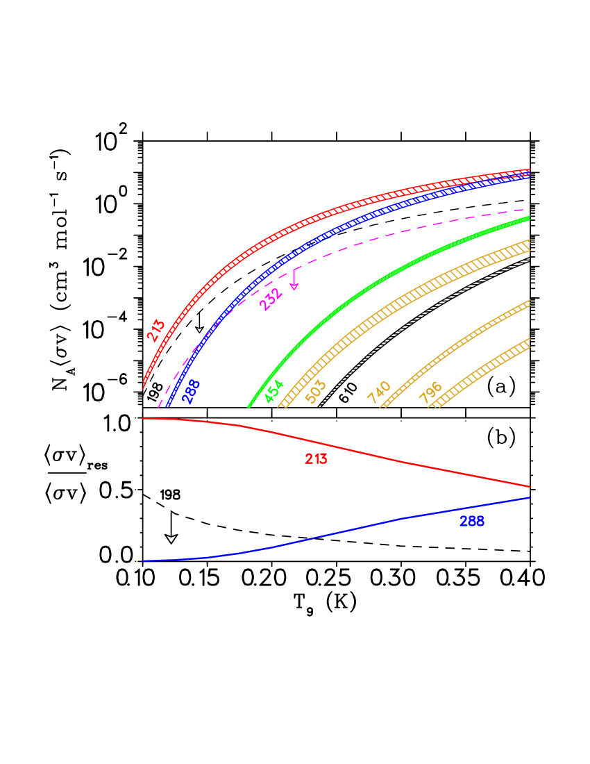
Figure 17: (color online) Thermonuclear ²²Na($p,\gamma)^{23}$Mg reaction rate as a function of temperature. Panel (a) shows contributions to the reaction rate from individual resonances labeled by $E_{p}$ (in keV), based on present measurements. Hatched regions represent 68% confidence levels (although the uncertainties are so small they may appear as solid lines), and dashed lines with arrows are 68% confidence level upper limits. Panel (b) shows the fractional contributions of selected resonances to the total rate, as calculated using the resonances illustrated in panel (a).

In Fig. 17 (a), we show the individual contributions to the thermonuclear rate for ²²Na($p,\gamma$), and panel (b) shows the relative contributions of selected resonances. As one can see, any contribution from the resonance at $E_{p}$ = 198 keV is less than that from the resonance at $E_{p}$ = 213 keV for all temperatures of interest to novae. Therefore, the resonance at $E_{p}=198$ keV does not dominate the reaction rate in this region, as Jenkins et al. Jenkins et al. (2004) proposed it might. Rather, the resonance at $E_{p}$ = 213 keV makes the most important contribution. Also, at the higher temperatures around 0.4 GK, the contribution of the 288-keV resonance becomes significant. The other resonance contributions are effectively negligible at nova temperatures.

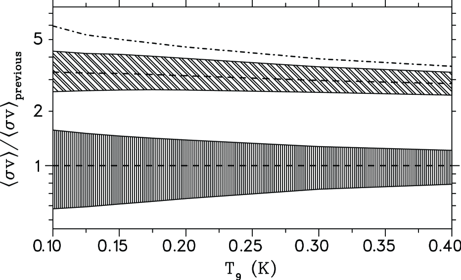
Figure 18: Ratio of present (slanted hatches) and previous (vertical hatches) Seuthe et al. (1990); Stegmüller et al. (1996) to previous thermonuclear ²²Na($p,\gamma)^{23}$Mg reaction rate as a function of temperature. Hatched areas represent 68% $C.L.$ error bands and dashed lines represent the central value, each relative to the previous central value. Both previous and present resonance strengths are listed in Table 4. Including the distributions for the resonances at $E_{p}=198$ and 232 keV increases the present upper limit to the dot-dashed line. The upper limit for the 198-keV resonance from Jenkins et al. Jenkins et al. (2004) has not been included in the previous rate.

Fig. 18 illustrates the total reaction rate relative to previous direct measurements Seuthe et al. (1990); Stegmüller et al. (1996), showing that our rate is inconsistent with previous work at all temperatures. The dashed line and hatched region in this figure do not include the distributions for proposed resonances at $E_{p}=$ 198 and 232 keV. The 232-keV resonance makes an insignificant contribution at all temperatures of interest to novae. However, although the 198-keV resonance was unobserved and an upper limit has been placed on its strength, including its potential contributions to the reaction rate has a non-negligible effect at low temperatures. Including the proposed resonances increases the upper limit of the reaction rate to the dot-dashed line shown in Fig. 18. Because of this difference, we have calculated the reaction rate for each of these two separate cases, and the values are shown in Table 5.

Table 5: Table of the thermonuclear ²²Na($p,\gamma)^{23}$Mg reaction rate, $R$, as a function of temperature, $T$, determined using the energies and strengths given in Table 4. Two distributions of rates were calculated, one of which includes the probability density functions from resonances at $E_{p}=198$ and 232 keV and one which does not. $R_{\rm central}$ is the 50% quantile of the distribution of rates at a given temperature, and $R_{\rm upper}$ and $R_{\rm lower}$ are the 16% and 84% quantiles, respectively. The units of the rate are cm³mol^-1s^-1.

	R (not including “198, 232”)			R (including “198, 232”)
$T_{9}$ (K)	$R_{\rm central}$	$R_{\rm lower}$	$R_{\rm upper}$	$R_{\rm central}$	$R_{\rm lower}$	$R_{\rm upper}$
0.01	2.0$\times 10^{-30}$	2.7$\times 10^{-31}$	1.5$\times 10^{-29}$	2.0$\times 10^{-30}$	2.7$\times 10^{-31}$	1.5$\times 10^{-29}$
0.02	5.5$\times 10^{-20}$	1.9$\times 10^{-20}$	1.6$\times 10^{-19}$	5.5$\times 10^{-20}$	1.9$\times 10^{-20}$	1.6$\times 10^{-19}$
0.03	2.6$\times 10^{-16}$	1.3$\times 10^{-16}$	5.6$\times 10^{-16}$	2.6$\times 10^{-16}$	1.3$\times 10^{-16}$	5.6$\times 10^{-16}$
0.04	4.6$\times 10^{-14}$	2.0$\times 10^{-14}$	1.1$\times 10^{-13}$	4.6$\times 10^{-14}$	2.1$\times 10^{-14}$	1.1$\times 10^{-13}$
0.05	1.4$\times 10^{-12}$	6.4$\times 10^{-13}$	3.1$\times 10^{-12}$	1.4$\times 10^{-12}$	6.4$\times 10^{-13}$	3.1$\times 10^{-12}$
0.06	1.4$\times 10^{-11}$	7.1$\times 10^{-12}$	2.8$\times 10^{-11}$	1.5$\times 10^{-11}$	7.7$\times 10^{-12}$	2.9$\times 10^{-11}$
0.07	1.8$\times 10^{-10}$	1.3$\times 10^{-10}$	2.5$\times 10^{-10}$	2.7$\times 10^{-10}$	2.0$\times 10^{-10}$	3.6$\times 10^{-10}$
0.08	6.2$\times 10^{-09}$	4.7$\times 10^{-09}$	8.2$\times 10^{-09}$	9.7$\times 10^{-09}$	7.2$\times 10^{-09}$	1.3$\times 10^{-08}$
0.09	1.3$\times 10^{-07}$	1.0$\times 10^{-07}$	1.8$\times 10^{-07}$	2.0$\times 10^{-07}$	1.5$\times 10^{-07}$	2.6$\times 10^{-07}$
0.10	1.6$\times 10^{-06}$	1.2$\times 10^{-06}$	2.1$\times 10^{-06}$	2.2$\times 10^{-06}$	1.7$\times 10^{-06}$	2.8$\times 10^{-06}$
0.15	2.3$\times 10^{-03}$	1.9$\times 10^{-03}$	3.0$\times 10^{-03}$	2.9$\times 10^{-03}$	2.4$\times 10^{-03}$	3.6$\times 10^{-03}$
0.2	8.5$\times 10^{-02}$	7.1$\times 10^{-02}$	1.1$\times 10^{-01}$	1.0$\times 10^{-01}$	8.4$\times 10^{-02}$	1.2$\times 10^{-01}$
0.3	3.1$\times 10^{+00}$	2.7$\times 10^{+00}$	3.7$\times 10^{+00}$	3.5$\times 10^{+00}$	3.0$\times 10^{+00}$	4.1$\times 10^{+00}$
0.4	1.9$\times 10^{+01}$	1.7$\times 10^{+01}$	2.2$\times 10^{+01}$	2.1$\times 10^{+01}$	1.8$\times 10^{+01}$	2.4$\times 10^{+01}$
0.5	5.9$\times 10^{+01}$	5.1$\times 10^{+01}$	6.7$\times 10^{+01}$	6.3$\times 10^{+01}$	5.4$\times 10^{+01}$	7.1$\times 10^{+01}$
0.6	1.3$\times 10^{+02}$	1.1$\times 10^{+02}$	1.4$\times 10^{+02}$	1.3$\times 10^{+02}$	1.2$\times 10^{+02}$	1.5$\times 10^{+02}$
0.7	2.3$\times 10^{+02}$	2.0$\times 10^{+02}$	2.5$\times 10^{+02}$	2.4$\times 10^{+02}$	2.1$\times 10^{+02}$	2.6$\times 10^{+02}$
0.8	3.6$\times 10^{+02}$	3.2$\times 10^{+02}$	4.0$\times 10^{+02}$	3.7$\times 10^{+02}$	3.3$\times 10^{+02}$	4.1$\times 10^{+02}$
0.9	5.4$\times 10^{+02}$	4.8$\times 10^{+02}$	5.9$\times 10^{+02}$	5.5$\times 10^{+02}$	5.0$\times 10^{+02}$	6.0$\times 10^{+02}$
1.0	7.5$\times 10^{+02}$	6.8$\times 10^{+02}$	8.1$\times 10^{+02}$	7.6$\times 10^{+02}$	6.9$\times 10^{+02}$	8.3$\times 10^{+02}$
1.5	2.2$\times 10^{+03}$	2.1$\times 10^{+03}$	2.4$\times 10^{+03}$	2.2$\times 10^{+03}$	2.1$\times 10^{+03}$	2.4$\times 10^{+03}$
2.0	3.9$\times 10^{+03}$	3.6$\times 10^{+03}$	4.2$\times 10^{+03}$	3.9$\times 10^{+03}$	3.6$\times 10^{+03}$	4.2$\times 10^{+03}$

Table 6: ²²Na yields from novae on ONe white dwarfs of various masses computed with SHIVA José and Hernanz (1998). The total mass ejected is given for each case, along with the mass fractions of ²²Na obtained using the central value of the previous Seuthe et al. (1990); Stegmüller et al. (1996) and both present ²²Na($p,\gamma)^{23}$Mg reaction rates compiled in Table 5. The factor given is the ratio of previous to respective present amounts of ²²Na ejected.

	$1.15M_{\odot}$	$1.25M_{\odot}$	$1.35M_{\odot}$
Meject (g)	4.9$\times 10^{28}$	3.8$\times 10^{28}$	9.0$\times 10^{27}$
Previous	1.6$\times 10^{-4}$	1.9$\times 10^{-4}$	5.9$\times 10^{-4}$
Present	8.8$\times 10^{-5}$	1.1$\times 10^{-4}$	4.1$\times 10^{-4}$
Factor	1.8	1.8	1.4
Present	7.8$\times 10^{-5}$	1.0$\times 10^{-4}$	3.8$\times 10^{-4}$
Factor	2.0	1.9	1.5

We can anticipate the general ramifications of the new rate on expected nucleosynthesis of ²²Na in ONe novae using post-processing network calculations because the total energy generation is not affected appreciably by the ²²Na($p,\gamma)$ reaction. Based on the one-zone calculations of Ref. Hix et al. (2003), a specific model indicates that the production of ²²Na is related inversely to the ²²Na($p,\gamma)$ reaction rate. The authors of Ref. Iliadis et al. (2001) also varied the rate by a factor of two using various one-zone models of novae to extract the effect. Using the information given in these references and our change in the reaction rate, the estimated abundance of ²²Na in novae is expected to be reduced by factors of 2 to 3 of what was previously expected, depending on white dwarf mass and composition. This will directly affect the expected flux of ²²Na gamma rays observed using orbiting gamma-ray telescopes.

In addition, the impact of our ²²Na$(p,\gamma)$ reaction rate on the amount of ²²Na ejected during nova outbursts has been tested through a series of hydrodynamic simulations: three evolutionary sequences of nova outbursts hosting ONe white dwarfs of 1.15, 1.25 and $1.35M_{\odot}$ have been computed with the spherically symmetric, Lagrangian, hydrodynamic code SHIVA, extensively used in the modeling of such explosions (see Ref. José and Hernanz (1998), for details). Results have been compared with those obtained in three additional hydrodynamic simulations, for the same white dwarf masses described above and same input physics except for the ²²Na$(p,\gamma)$ rate, which was derived from Refs. Stegmüller et al. (1996); Seuthe et al. (1990). The network used for additional reaction rates is the relevant subset of that used in Ref. José et al. (2010). The estimated ²²Na yields (mass-averaged mass fractions in the overall ejected shells) are listed in Table 6, which clearly shows that the impact of the central value of new rate roughly translates into lower ²²Na abundances by a factor up to $\sim$ 2 with respect to previous estimates. This, in turn, directly affects the chances to potentially detect the 1275-keV gamma-ray line from ²²Na decay, decreasing the maximum detectability distances by a factor $\sim 1.4$. The inclusion of the 198- and 232-keV distributions in the rate does not appreciably alter this factor.

The results from one-zone post-processing network calculations and full hydrodynamic simulations using SHIVA are complementary. The post-processing approach mimics the processes that occur in the deepest envelope layers, whereas the hydrodynamic simulations average the yields over all ejected shells. Convection also plays a critical role, supplying freshly, unburned material from external shells into the innermost one (and vice versa), and these effects cannot be simulated in a post-processing framework. As a result of the more realistic physics in the hydrodynamic model, the composition of the innermost shell is diluted by the compositions of the outermost ones. On the other hand, the post-processing calculations cover various nova models, a wider range of nova masses and compositions, and show that the correlation between the ²²Na($p,\gamma)$ rate and ²²Na production is robust even when other reaction rates are simultaneously varied. It seems reasonable to assume that the magnitude of the dilution from the hydrodynamic models ($\approx 25\%$) applies generally to all of the post-processing results.

VI Conclusions

We have measured the resonance strengths, energies, and branches of the ²²Na($p,\gamma)^{23}$Mg reaction directly and absolutely. Our method improved upon past measurements in several ways. The use of integrated yields makes the results independent of absolute stopping power calculations and is far more robust than using peak yields. We also utilized isotopically-pure, implanted targets that demonstrated nearly zero loss during bombardment. HPGe detectors exhibit excellent energy resolution, providing the ability to use narrow energy windows, and anticoincidence shields enabled suppression of the cosmic ray background. Absolute detector efficiency was also vital, which we determined by fusing measurement and simulation. Finally, the rastering of the beam across the target not only aided in maintaining target integrity, but also removed the requirement of detailed knowledge of the target distribution. A determination of the beam density was mandatory and was ascertained by both measurement and modeling. As a consequence of the aforementioned points, our results should be substantially more reliable than previous measurements.

By exploiting these advantages, our measurement has shown that four previously measured resonance strengths are 2.4 to 3.2 times higher than previously reported Seuthe et al. (1990); Stegmüller et al. (1996). Jenkins et al. also proposed that a new ²²Na($p,\gamma$) resonance with $E_{p}=$ 198 keV could dominate this reaction rate and have consequences for novae Jenkins et al. (2004). We have demonstrated that this is not the case, and that the main contributions arise from the resonance at $E_{p}$ = 213 keV. As a result of the higher resonance strengths, the estimated flux of ²²Na gamma rays from novae is expected to be about a factor of 2 less than what was previously expected, determined by using both post-processing network calculations and hydrodynamic simulations. The lack of observational evidence of ²²Na in the cosmos is consistent with the previous reaction rate; however, the present rate makes detection $\sim$ 1.4 times more difficult to detect.