Diffusive properties of persistent walks on cubic lattices with application to periodic Lorentz gases

Abstract

We calculate the diffusion coefficients of persistent random walks on cubic and hypercubic lattices, where the direction of a walker at a given step depends on the memory of one or two previous steps. These results are then applied to study a billiard model, namely a three-dimensional periodic Lorentz gas. The geometry of the model is studied in order to find the regimes in which it exhibits normal diffusion. In this regime, we calculate numerically the transition probabilities between cells to compare the persistent random-walk approximation with simulation results for the diffusion coefficient.

1 Introduction

Problems dealing with the persistence of motion of tracer particles – that is, the tendency to continue or not in the same direction at a scattering event – are encountered in many areas of physics; see e.g. [1] and references therein. We are specifically interested in the effect of persistence for the motion of random walkers on regular lattices.

The diffusive properties of persistent random walks on two-dimensional regular lattices were the subject of a previous paper by two of the present authors [2]. There, we presented a theory making use of the symmetries of such lattices to derive the transport coefficients of walks with a two-step memory. In the first part of the present paper, we extend this theory to hyper-cubic lattices in arbitrary dimensions, which is possible by describing the geometry of the lattices in a suitable way.

Persistence effects naturally arise in the context of deterministic diffusion [3, 4, 5, 6], which is concerned with the interplay between dynamical properties at the microscopic scale and transport properties at the macroscopic scale. A variety of different techniques are now available, which rely on the chaotic properties of model systems to describe their macroscopic properties [7], [8, chap. 25]. In particular, periodic Lorentz gases and related models, such as multi-baker maps, are simple deterministic dynamical systems with strong chaotic properties which also exhibit diffusive regimes. Although the transport coefficients of these models can be expressed formally in terms of the microscopic dynamical properties, actually computing them is usually difficult, with the exception of some of the simplest toy models [9, 10, 11]. One reason for this is that memory effects can remain important, in spite of the chaotic character of the underlying dynamics.

The diffusive properties of these models therefore provide ideal applications of the formalism presented in this paper. An example of this was illustrated in reference [12], for a class of two-dimensional periodic billiard tables. Extending these results, in this paper we apply the formalism to model the diffusive properties of higher-dimensional periodic Lorentz gases.

The diffusive properties of the three-dimensional periodic Lorentz gas, which consists of the free motion of independent tracer particles in a cubic array of spherical obstacles, are interesting in their own right. In two spatial dimensions, the existence of diffusive regimes in such systems has been rigorously established [13, 14]. It relies on the finite-horizon property, which requires that the system admits no ballistic trajectories, i.e. those which never collide with any obstacle. In this case, it is possible to change scales from microscopic to macroscopic, reducing the complicated motion of tracer particles at the microscopic level to a diffusive equation at the macroscopic level. When the horizon is infinite on the other hand, there is rather a weakly superdiffusive process, with mean-squared displacement growing like $t\log t$ [15, 16], as recently shown rigorously in [17].

The necessity of finite horizon to have normal diffusion in two dimensions led to the idea that this was also necessary in three dimensions – see, for example, reference [18]. Recently, however, it was argued by one of the present authors [19] that in higher-dimensional billiards, normal diffusion, by which we mean an asymptotically linear growth in time of the mean-squared displacement, may arise even in the absence of finite horizon. In fact, three different types of horizon can be identified in the three-dimensional periodic Lorentz gas. The key observation is that it is only “planar” gaps – those with infinite extension in two dimensions – which induce anomalous diffusion. If there are only “cylindrical” gaps, whose extension is limited to a single dimension, then the available space in which particles can move ballistically is limited. This leads to a decay of correlations which is fast enough to give normal diffusion at the level of the mean-squared displacement, although higher moments of the displacement distribution may be non-Gaussian [19].

The paper is organized as follows. Section 2 describes the computation of the transport coefficient of walks on hypercubic lattices with one and two-step memories. In the second part of this paper, we apply this formalism to the diffusive regimes of the three-dimensional periodic Lorentz gas. In section 3, we give a detailed description of the three-dimensional periodic Lorentz gas introduced in reference [19], in particular delimiting the regimes with qualitatively different behaviour in parameter space. We then apply the results on persistent random walks to the diffusive regimes of this model in section 4. Conclusions are drawn in section 5.

2 Persistent random walks on cubic lattices

In this section, we describe a way to incorporate the specific geometry of cubic and hyper-cubic lattices in the framework presented in reference [2] for calculating diffusion coefficients for persistent random walks on lattices.

We start by considering the motion of independent walkers on a regular cubic lattice in three dimensions. Given their initial position $\bi{r}_{0}$ at time $t=0$, the walkers’ trajectories are specified by the sequence $\{\bi{v}_{0},\ldots,\bi{v}_{n}\}$ of their successive displacements. Here we consider dynamics in discrete time, so that the time sequences are simply assumed to be incremented by identical time steps $\tau$ as the walkers move from site to site. In the sequel we will loosely refer to the displacement vectors as velocity vectors; they are in fact dimensionless unit vectors.

The sequence of successive displacements is determined by the underlying dynamics, whether deterministic or stochastic. At the coarse level of description of the lattice dynamics, this is interpreted as a persistent type of random walk, where some memory effects are accounted for: the probability that the $n$th step is taken in the direction $\bi{v}_{n}$ depends on the past history $\bi{v}_{n-1},\bi{v}_{n-2},\ldots$.

The quantity of interest here is the diffusion coefficient $D$ of such persistent processes, which measures the linear growth in time of the mean-squared displacement of walkers. This can be written in terms of velocity autocorrelations using the Taylor–Green–Kubo expression:

$$D=\frac{\ell^{2}}{2d\tau}\left[1+2\lim_{k\to\infty}\sum_{n=1}^{k}\langle\bi{v}_{0}\cdot\bi{v}_{n}\rangle\right]\,,$$ (2.1)

where $d$ denotes the dimensionality of the lattice, here $d=3$, and $\ell$ is the lattice spacing. The (dimensionless) velocity autocorrelations are computed as averages $\langle\cdot\rangle$ over the equilibrium distribution, denoted by $\mu$, of the underlying process, so that the problem reduces to computing the quantities

$$\langle\bi{v}_{0}\cdot\bi{v}_{n}\rangle=\sum_{\bi{v}_{0},\ldots,\bi{v}_{n}}\bi{v}_{0}\cdot\bi{v}_{n}\,\mu(\{\bi{v}_{0},\ldots,\bi{v}_{n}\})\,.$$ (2.2)

Following the approach of reference [2], we wish to compute the terms in this sum, and hence the corresponding diffusion coefficient (2.1), for three different types of random walks, namely those with zero-step, single-step and two-step memories. These cases all involve factorisations of the measure $\mu(\{\bi{v}_{0},\ldots,\bi{v}_{n}\})$ into products of probability measures which depend on a number of velocity vectors, equal to the number of steps of memory of the walkers. These measures will be denoted by $p$ throughout.

The schemes we outline below allow to write equation (2.2) as a sum of powers of matrices, so that (2.1) boils down to a geometric series, which can then be resummed to obtain an expression for the diffusion coefficient that is readily computable given the probabilities that characterise the allowed transitions in the process.

2.1 Description of geometry of cubic lattices

It is first necessary to find a succinct description of the geometry of the cubic lattices that we wish to study. The six directions of the three-dimensional cubic lattice and corresponding displacement vectors are specified in terms of the unit vectors $\bi{e}_{i}$ of a Cartesian coordinate system as $\pm\bi{e}_{i}$, $i=1,2,3$.

The crucial property required for the application of our method is that all of these unit vectors can be obtained by repeated application of a single transformation $\mathsf{G}$, which generates the cyclic group

$$\mathcal{G}\equiv\{\mathsf{G}_{i}\equiv\mathsf{G}^{i},\quad i=0,\ldots,5\}.$$ (2.3)

One possible choice of $\mathsf{G}$ gives the following group elements:

$$\eqalign{\mathsf{G}_{1}=-\mathsf{G}_{4}=\mathsf{G}=\left(\begin{array}[]{ccc}0&0&-1\\ 1&0&0\\ 0&1&0\end{array}\right),\\ \mathsf{G}_{2}=-\mathsf{G}_{5}=\mathsf{G}^{2}=\left(\begin{array}[]{ccc}0&-1&0\\ 0&0&-1\\ 1&0&0\end{array}\right),\\ \mathsf{G}_{3}=-\mathsf{G}_{0}=\mathsf{G}^{3}=\left(\begin{array}[]{ccc}-1&0&0\\ 0&-1&0\\ 0&0&-1\end{array}\right).}$$ (2.4)

Figure 1 displays the six possible directions of a walker on this lattice, numbered according to repeated iterations by $\mathsf{G}$. Thus a walker with incoming direction $\bi{e}_{1}$, indicated by the arrow, can be deflected to any of the six directions $\mathsf{G}^{i}\bi{e}_{1}$, $i=0,\ldots,5$, corresponding respectively to $\bi{e}_{1}$, $\bi{e}_{2}$, $\bi{e}_{3}$, $-\bi{e}_{1}$, $-\bi{e}_{2}$, and $-\bi{e}_{3}$.

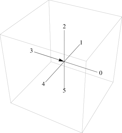
Figure 1: The possible directions of motion on a cubic lattice, labelled from $0$ to $5$ relative to the incoming direction shown by the arrow. These directions are obtained by successive applications of the transformation $\mathsf{G}$ given in equation (2.4).

A similar transformation $\mathsf{G}$ can easily be identified for a walk on a $d$-dimensional hyper-cubic lattice:

$$\mathsf{G}=\left(\begin{array}[]{ccccc}0&0&\cdots&0&-1\\ 1&0&\cdots&0&0\\ 0&1&\cdots&0&0\\ \vdots&&\ddots&&\vdots\\ 0&0&\cdots&1&0\end{array}\right),$$ (2.5)

which maps the unit vectors onto the $2d$-cycle $\bi{e}_{1}\mapsto\bi{e}_{2}\mapsto\cdots\mapsto\bi{e}_{d}\mapsto-\bi{e}_{1}\mapsto\cdots\mapsto-\bi{e}_{d}$.

2.2 No-Memory Approximation (NMA)

We now proceed to calculate the diffusion coefficient (2.1) for random walks with different memory lengths. The simplest case is that of a Bernoulli process for the velocity trials, so that the walkers have no memory of their history as they proceed to their next position. The probability measure $\mu$ thus factorises:

$$\mu(\{\bi{v}_{0},\ldots,\bi{v}_{n}\})=\prod_{i=0}^{n}p(\bi{v}_{i})\,.$$ (2.6)

Given that the lattice is rotation invariant and that $p$ is uniform, the velocity autocorrelation (2.2) vanishes:

$$\langle\bi{v}_{0}\cdot\bi{v}_{n}\rangle=\delta_{n,0}\,.$$ (2.7)

The diffusion coefficient of the random walk without memory is then given by

$$D_{\mathrm{NMA}}=\frac{\ell^{2}}{2d\tau}\,.$$ (2.8)

2.3 One-Step Memory Approximation (1-SMA)

We now assume that the velocity vectors obey a Markov process, for which $\bi{v}_{n}$ takes on different values according to the velocity at the previous step $\bi{v}_{n-1}$. We may then write

$$\mu(\{\bi{v}_{0},\ldots,\bi{v}_{n}\})=\prod_{i=1}^{n}P(\bi{v}_{i}|\bi{v}_{i-1})p(\bi{v}_{0})\,.$$ (2.9)

Here, $P(\bi{v}^{\prime}|\bi{v})$ denotes the one-step conditional probability that the walker moves with displacement $\bi{v}^{\prime}$, given that it made a displacement $\bi{v}$ at the previous step.

Considering for definiteness the three-dimensional lattice and using the elements of the group $\mathcal{G}$, we express each velocity vector $\bi{v}_{k}$ in terms of the first one, $\bi{v}_{0}$, as $\bi{v}_{k}=\mathsf{G}^{i_{k}}\bi{v}_{0}$, where each $i_{k}\in\{0,\ldots,5\}$. Substituting this into the expression for the velocity autocorrelation $\langle\bi{v}_{0}\cdot\bi{v}_{n}\rangle$, equation (2.2), we obtain, using the factorisation (2.9),

$$\sum_{\bi{v}_{0},\ldots,\bi{v}_{n}}\bi{v}_{0}\cdot\bi{v}_{n}\,\prod_{i=1}^{n}P(\bi{v}_{i}|\bi{v}_{i-1})p(\bi{v}_{0})=\sum_{i_{0},\ldots,i_{n}=1}^{6}\bi{v}_{0}\cdot\mathsf{G}^{i_{n}}\bi{v}_{0}\,\mathsf{m}_{i_{n},i_{n-1}}\cdots\mathsf{m}_{i_{1},i_{0}}\mathsf{p}_{i_{0}}\,.$$ (2.10)

In this expression,

$$\mathsf{m}_{i_{n},i_{n-1}}\equiv P(\mathsf{G}^{i_{n}}\bi{v}_{0}|\mathsf{G}^{i_{n-1}}\bi{v}_{0})$$ (2.11)

are the elements of the stochastic matrix $\mathsf{M}$ of the Markov chain associated to the persistent random walk, and $\mathsf{p}_{i}\equiv p(\bi{e}_{i})$ are the elements of its invariant (equilibrium) distribution, denoted $\mathsf{P}$, evaluated with a velocity in the $i$th lattice direction. The invariance of $\mathsf{P}$ is expressed as $\sum_{j}\mathsf{m}_{i,j}\mathsf{p}_{j}=\mathsf{p}_{i}$. The same notations were used in [2] and will be used throughout this article.

The terms involving $\mathsf{M}$ in (2.10) constitute the matrix product of $n$ copies of $\mathsf{M}$. Furthermore, since the invariant distribution is uniform over the lattice directions, we can choose an arbitrary direction for $\bi{v}_{0}$, and hence write

$$\langle\bi{v}_{0}\cdot\bi{v}_{n}\rangle =\bi{v}_{0}\cdot\bi{v}_{0}\,\mathsf{m}^{(n)}_{1,1}+\bi{v}_{0}\cdot\mathsf{G}\bi{v}_{0}\,\mathsf{m}^{(n)}_{2,1}+\cdots+\bi{v}_{0}\cdot\mathsf{G}^{5}\bi{v}_{0}\,\mathsf{m}^{(n)}_{6,1}\,,$$ (2.12)

$$=\mathsf{m}^{(n)}_{1,1}-\mathsf{m}^{(n)}_{4,1}$$

where $\mathsf{m}^{(n)}_{i,j}$ denote the elements of $\mathsf{M}^{n}$.

The actual value of the diffusion coefficient depends on the probabilities $P(\mathsf{G}^{j}\bi{v}|\bi{v})$, which are parameters of the model, subject to the constraints $\sum_{j}P(\mathsf{G}^{j}\bi{v}|\bi{v})=1$. To simplify the notation, we assume rotational invariance of the process, i.e. independence with respect to the value of $\bi{v}$, and we denote the conditional probabilities of these walks by $P_{j}\equiv P(\mathsf{G}^{j}\bi{v}|\bi{v})$, where $j=0,\ldots,5$.

The transition matrix $\mathsf{M}$ given by (2.11) is thus the cyclic matrix

$$\mathsf{M}=\left(\begin{array}[]{c@{\enspace}c@{\enspace}c@{\enspace}c@{\enspace}c@{\enspace}c}P_{0}&P_{1}&P_{2}&P_{3}&P_{4}&P_{5}\\ P_{5}&P_{0}&P_{1}&P_{2}&P_{3}&P_{4}\\ P_{4}&P_{5}&P_{0}&P_{1}&P_{2}&P_{3}\\ P_{3}&P_{4}&P_{5}&P_{0}&P_{1}&P_{2}\\ P_{2}&P_{3}&P_{4}&P_{5}&P_{0}&P_{1}\\ P_{1}&P_{2}&P_{3}&P_{4}&P_{5}&P_{0}\end{array}\right)\,.$$ (2.13)

The matrix $\mathsf{M}^{n}$ shares the same property of cyclicity, so that it also has only six distinct entries. It is thus possible to proceed along the lines described in [2] and obtain the recurrence relation

$$\left(\begin{array}[]{c}\mathsf{m}^{(n)}_{1,1}-\mathsf{m}^{(n)}_{4,1}\\ \mathsf{m}^{(n)}_{2,1}-\mathsf{m}^{(n)}_{5,1}\\ \mathsf{m}^{(n)}_{3,1}-\mathsf{m}^{(n)}_{6,1}\end{array}\right) =\left(\begin{array}[]{c@{\enspace}c@{\enspace}c}P_{0}-P_{3}&P_{1}-P_{4}&P_{2}-P_{5}\\ P_{5}-P_{2}&P_{0}-P_{3}&P_{1}-P_{4}\\ P_{4}-P_{1}&P_{5}-P_{2}&P_{0}-P_{3}\end{array}\right)\left(\begin{array}[]{c}\mathsf{m}^{(n-1)}_{1,1}-\mathsf{m}^{(n-1)}_{4,1}\\ \mathsf{m}^{(n-1)}_{2,1}-\mathsf{m}^{(n-1)}_{5,1}\\ \mathsf{m}^{(n-1)}_{3,1}-\mathsf{m}^{(n-1)}_{6,1}\end{array}\right),$$ (2.23)

$$=\left(\begin{array}[]{c@{\enspace}c@{\enspace}c}P_{0}-P_{3}&P_{1}-P_{4}&P_{2}-P_{5}\\ P_{5}-P_{2}&P_{0}-P_{3}&P_{1}-P_{4}\\ P_{4}-P_{1}&P_{5}-P_{2}&P_{0}-P_{3}\end{array}\right)^{n-1}\left(\begin{array}[]{c}P_{0}-P_{3}\\ P_{1}-P_{4}\\ P_{2}-P_{5}\end{array}\right).$$ (2.30)

[Note that the left-hand side of this equation was chosen to reduce the size of the matrix involved and to calculate the element required in (2.12).] As a consequence, we can write for the velocity autocorrelation (2.12)

$$\eqalign{\langle}\bi{v}_{0}\cdot\bi{v}_{n}\rangle=\big{(}1\enspace 0\enspace 0\big{)}\left(\begin{array}[]{c@{\enspace}c@{\enspace}c}P_{0}-P_{3}&P_{1}-P_{4}&P_{2}-P_{5}\\ P_{5}-P_{2}&P_{0}-P_{3}&P_{1}-P_{4}\\ P_{4}-P_{1}&P_{5}-P_{2}&P_{0}-P_{3}\end{array}\right)^{n-1}\left(\begin{array}[]{c}P_{0}-P_{3}\\ P_{1}-P_{4}\\ P_{2}-P_{5}\end{array}\right),$$ (2.31)

and thus obtain the expression of the diffusion coefficient (2.1) as

$$\frac{D_{\mathrm{1SMA}}}{D_{\mathrm{NMA}}}=\left[1+2\Big{(}1\enspace 0\enspace 0\Big{)}\left(\begin{array}[]{c@{\enspace}c@{\enspace}c}\scriptstyle 1+P_{3}-P_{0}&\scriptstyle P_{4}-P_{1}&\scriptstyle P_{5}-P_{2}\\ \scriptstyle P_{2}-P_{5}&\scriptstyle 1+P_{3}-P_{0}&\scriptstyle P_{4}-P_{1}\\ \scriptstyle P_{1}-P_{4}&\scriptstyle P_{2}-P_{5}&\scriptstyle 1+\scriptstyle P_{3}-P_{0}\end{array}\right)^{-1}\left(\begin{array}[]{c}P_{0}-P_{3}\\ P_{1}-P_{4}\\ P_{2}-P_{5}\end{array}\right)\right],$$ (2.32)

by using the result that $\sum_{n=0}^{\infty}\mathsf{A}^{n}=(\mathsf{I}-\mathsf{A})^{-1}$, where $\mathsf{I}$ is the identity matrix, for a square matrix $\mathsf{A}$ whose eigenvalues are all strictly less than $1$ in modulus,

This result easily generalises to a hyper-cubic lattice in any dimension $d$. Note also that for a symmetric process, in which $P_{1}=P_{4}$ and $P_{2}=P_{5}$, we recover the diffusion coefficient

$$D_{\mathrm{1SMA}}=D_{\mathrm{NMA}}\frac{1+P_{0}-P_{3}}{1-P_{0}+P_{3}},$$ (2.33)

in agreement with the result stated in [2].

2.4 Two-Step Memory Approximation (2-SMA)

Let us now suppose that the velocity vectors obey a random process for which the probability of $\bi{v}_{n}$ takes on different values according to the velocities at the two previous steps, $\bi{v}_{n-1}$ and $\bi{v}_{n-2}$, so that we may write

$$\mu(\{\bi{v}_{0},\ldots,\bi{v}_{n}\})=\prod_{i=2}^{n}P(\bi{v}_{i}|\bi{v}_{i-1},\bi{v}_{i-2})p(\bi{v}_{0},\bi{v}_{1})\,.$$ (2.34)

The velocity autocorrelation (2.2) function is then

$$\langle\bi{v}_{0}\cdot\bi{v}_{n}\rangle=\sum_{\{\bi{v}_{n},\ldots,\bi{v}_{0}\}}\bi{v}_{0}\cdot\bi{v}_{n}\,\prod_{i=2}^{n}P(\bi{v}_{i}|\bi{v}_{i-1},\bi{v}_{i-2})p(\bi{v}_{0},\bi{v}_{1})\,.$$ (2.35)

Since the probability transitions $P(\bi{v}_{i}|\bi{v}_{i-1},\bi{v}_{i-2})$ have symmetries similar to those used in reference [2], the computation of equation (2.35) reduces to an expression very similar to that found there for walks on one- and two-dimensional lattices. The details of the derivation are a bit more involved than the one-step memory persistent walks, so we will limit ourselves to stating the results.

Letting $z=2d$ denote the coordination number of the lattice, and writing $P_{j,k}\equiv P(\mathsf{G}^{z-k}\mathsf{G}^{z-j}\bi{v}|\mathsf{G}^{z-j}\bi{v},\bi{v})$, which is the conditional probability of making a displacement $\bi{v}$ given that the two preceding displacements were successively $\mathsf{G}^{j}\mathsf{G}^{k}\bi{v}$ and $\mathsf{G}^{k}\bi{v}$, we define the $z\times z$ matrix

$$K(\phi)\equiv\left(\begin{array}[]{c@{\enspace}c@{\enspace}c@{\enspace}c}\scriptstyle P_{00}&\scriptstyle P_{10}&\scriptstyle\cdots&\scriptstyle P_{z-1,0}\\ \scriptstyle\phi P_{01}&\scriptstyle\phi P_{11}&\scriptstyle\cdots&\scriptstyle\phi P_{z-1,1}\\ \scriptstyle\vdots&\scriptstyle\vdots&\scriptstyle\ddots&\scriptstyle\vdots\\ \scriptstyle\phi^{z-1}P_{0,z-1}&\scriptstyle\phi^{z-1}P_{1,z-1}&\scriptstyle\cdots&\scriptstyle\phi^{z-1}P_{z-1,z-1}\end{array}\right).$$ (2.36)

The argument $\phi$ in this expression is a complex number such that $\phi^{z}=1$. In the case of two-dimensional lattices, only two of these roots are relevant, corresponding to the complex exponential of the smallest angle between two lattice vectors, $\phi=\exp(\pm 2i\pi/z)$. For hyper-cubic lattices in arbitrary dimensions, however, we must consider a priori all the $z$ possible roots of unity, $\phi_{j}\equiv\exp(2i\pi j/z)$, $j=0,\ldots,z-1$.

A direct calculation of (2.35) shows that the velocity autocorrelation takes the form

$$\langle\bi{v}_{0}\cdot\bi{v}_{n}\rangle=\Big{(}1\cdots 1\Big{)}\left[\sum_{j=0}^{z-1}a_{j}K(\phi_{j})^{n-1}\mathrm{diag}(1,\phi_{j},\ldots,\phi_{j}^{z-1})\right]\left(\begin{array}[]{c}\mathsf{p}_{1}\\ \vdots\\ \mathsf{p}_{z}\end{array}\right),$$ (2.37)

where $\mathrm{diag}(1,\phi_{j},\ldots,\phi_{j}^{z-1})$ denotes the matrix with elements listed on the main diagonal and $0$ elsewhere. For the three-dimensional cubic lattice, the coefficients $a_{j}$ are found to be

$$\eqalign{a_{0}=a_{2}=a_{4}=0,\\ a_{1}=a_{3}=a_{5}=2,}$$ (2.38)

which compares to $a_{1}=a_{3}=2$ and $a_{0}=a_{2}=0$ in the case of the two-dimensional square lattice [2]. In the case of a $d$-dimensional hyper-cubic lattice, this generalises to

$$\eqalign{a_{2j}=0,\quad j=0,\ldots,d-1,\\ a_{2j+1}=2,\quad j=0,\ldots,d-1,}$$ (2.39)

The diffusion coefficient of a two-step memory persistent random walk on a $d$-dimensional hyper-cubic lattice is thus

$$\frac{D_{\mathrm{2SMA}}}{D_{\mathrm{NMA}}}=1+4\Big{(}1\cdots 1\Big{)}\left\{\sum_{j=1}^{d}[I_{z}-K(\phi_{2j-1})]^{-1}\mathrm{diag}(1,\phi_{2j-1},\ldots,\phi_{2j-1}^{z-1})\right\}\left(\begin{array}[]{c}\mathsf{p}_{1}\\ \vdots\\ \mathsf{p}_{z}\end{array}\right),$$ (2.43)

(2.44)

where $I_{z}$ denotes the $z\times z$ identity matrix.

3 Three-dimensional periodic Lorentz gas

Equations (2.8), (2.32) and (2.44) can be put to the test to probe the diffusive regimes of periodic Lorentz gases. The diffusive motion of the tracers results from the chaotic nature of the microscopic dynamics and the fast decay of correlations, which are in turn due to the convex nature of the obstacles. Taking into consideration the different diffusive regimes of these models, which, as we argued earlier, depend on the nature of their horizon, we investigate how the microscopic dynamical properties of the system determine the diffusion coefficient.

Machta and Zwanzig [20] addressed this issue in a particular limiting case, showing that, in the limit where the obstacles are so close together that a tracer will remain localised on ekach lattice site for a very long time (compared to the mean time separating two collision events), the process of diffusion on the Lorentz gas is well approximated by the dimensional prediction (2.8), where the lattice spacing $\ell$ is the distance separating two neighbouring obstacles and $\tau$ is the trapping time, which can be computed in terms of the geometry of the billiard as a simple consequence of ergodicity. That is to say, when the geometry of the billiard is such that two neighbouring disks nearly touch, the Lorentz gas is well approximated by a Bernoulli process, modeling the random hopping of tracers from cell to cell, with time- and length-scales specified according to the geometry of the billiard.

Different approximation schemes have been proposed to go beyond this zeroth-order approximation and account for corrections to it [21, 22]; see, in particular, reference [23] for an overview. A consistent approach to understanding the effect of these corrections in two-dimensional diffusive billiards was described in [12]. The idea is to approximate the hopping process of tracer particles by persistent random walks with finite memory, and thus estimate the diffusion coefficient of the billiard by the two-dimensional lattice equivalents of the one- or two-step formulas (2.32) and (2.44).

We discuss below the transposition of these results to the diffusive regimes of the three-dimensional periodic Lorentz gas.

3.1 Geometry of simple three-dimensional periodic Lorentz gas model

We begin with a detailed description of the geometry and the different horizon regimes of the system studied in reference [19]; additional details are given in reference [24].

The model consists of a three-dimensional (3D) periodic Lorentz gas constructed out of cubic unit cells of side length $\ell$, having eight “outer” spheres of radius $\rho_{\mathrm{out}}\ell$ at its corners and a single “inner” sphere of radius $\rho_{\mathrm{in}}\ell$ at its centre – see figure 2. The infinitely-extended periodic structure formed in this way is symmetric under interchange of $\rho_{\mathrm{in}}$ and $\rho_{\mathrm{out}}$; without loss of generality, we take $\rho_{\mathrm{out}}\geq\rho_{\mathrm{in}}$.

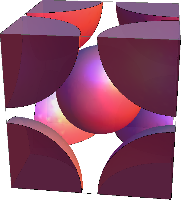
Figure 2: Geometry of the obstacles in a single cell of the 3D periodic Lorentz gas model for $\rho_{\mathrm{out}}=0.45\ell$ and $\rho_{\mathrm{in}}=0.30\ell$, in the cylindrical-horizon regime.

This model seems to be the simplest one which allows a finite horizon, although this is possible only when the spheres are permitted to overlap. It is known that finite-horizon periodic Lorentz gases with non-overlapping spheres in fact exist in any dimension [25], but we are not aware of any explicit constructions of such models, even in the case of three dimensions.

Lattice of outer spheres

The spheres of radius $\rho_{\mathrm{out}}\ell$ form a simple cubic lattice. This lattice has the following properties:

• When $\rho_{\mathrm{out}}<1/2$, the spheres are disjoint. In this case, there are free planes [25] in the structure, that is, infinite planes which do not intersect any of the spheres, in particular there are free planes centered on the faces of the unit cell. In this case, we say that there is a planar horizon (PH). When $\rho_{\mathrm{out}}$ is small, there are additional planes at different diagonal angles, analogously to the two-dimensional infinite-horizon Lorentz gas [15, 16, 17].

• When $\rho_{\mathrm{out}}>1/2$, the spheres overlap, thereby automatically blocking all planes. The overlaps (intersections) of the spheres partially cover the faces of the cubes, leaving a space in between which acts as an exit towards the adjacent cell.

• When $\rho_{\mathrm{out}}\geq 1/\sqrt{2}$, the overlaps completely cover the faces of the unit cell, so that it is no longer possible to exit the cell.

• When $\rho_{\mathrm{out}}\geq\sqrt{3}/2$, all of space is covered, and it is no longer possible to define a billiard dynamics.

Conditions for normal diffusion: cylindrical horizon

As shown in reference [19], the necessary and sufficient condition to have normal diffusion is that all free planes are blocked; if there are free planes, then the diffusion is weakly anomalous. The conditions to block all planes are as follows.

• All free planes are automatically blocked for $\rho_{\mathrm{out}}\geq 1/2$, when the $\rho_{\mathrm{out}}$-spheres overlap.

• If the $\rho_{\mathrm{out}}$-spheres do not overlap, then it is necessary to introduce the $\rho_{\mathrm{in}}$-sphere to block planes which are parallel to the faces of the unit cell. For this blocking to occur, we need $\rho_{\mathrm{in}}\geq 1/2-\rho_{\mathrm{out}}$.

• Furthermore, we must also block diagonal planes at $45$ degree angles, which requires that $\rho_{\mathrm{out}}\geq 1/(2\sqrt{2})$ or $\rho_{\mathrm{in}}\geq 1/(2\sqrt{2})$.

If all of these conditions are satisfied, then we no longer have free planes, but may have free cylinders (“cylindrical gaps”) in the structure; we then say that there is a cylindrical horizon (CH).

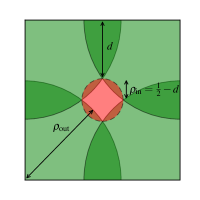
(a) Face of unit cell

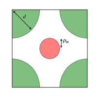
(b) Mid-plane of unit cell

Figure 3: Geometry of the 3D periodic Lorentz gas. (a) Cross-section of the unit cell in one of its faces. The overlapping outer spheres of radius $\rho_{\mathrm{out}}>1/2$, give rise to four overlapping discs (shown in green); the maximum width of their overlap is denoted $d$. The central disc (red) shows the minimum radius $\rho_{\mathrm{in}}=1/2-d$ of the central sphere such that its projection covers the gap between the $\rho_{\mathrm{out}}$-discs on the face. (b) Geometry of the mid-plane of a unit cell for parameters giving a finite horizon. The outer discs are cross-sections of the overlaps of the outer $\rho_{\mathrm{out}}$-spheres, and have radius $d$ equal to the overlap parameter in (a). The inner disc is the cross-section of the inner $\rho_{\mathrm{in}}$-sphere.

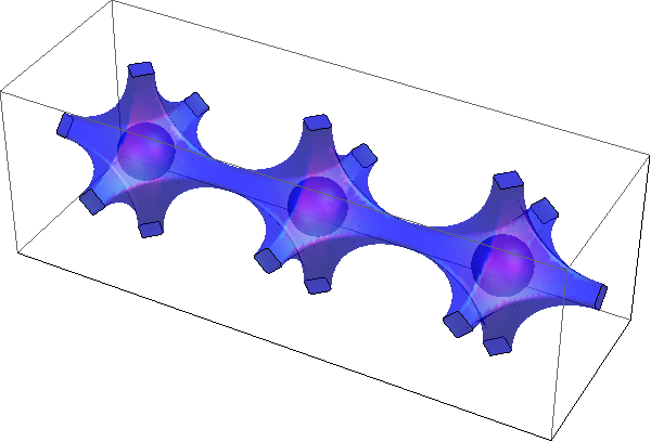
Figure 4: Finite horizon can be achieved in a three-dimensional lattice, provided the spheres are allowed to overlap. Here the available space for diffusing particles is shown for parameter values $\rho_{\mathrm{out}}=0.65\ell$ and $\rho_{\mathrm{in}}=0.15\ell$ (in the FH1 region) in an unfolded channel.

Conditions for finite horizon

Stronger statistical properties – e.g. faster decay of correlations – may be expected when there is a finite horizon [18, 19], i.e. where the length of free paths between collisions with obstacles is bounded above. To obtain this, not only all planar gaps, but also all cylindrical gaps must be blocked, i.e. all holes viewed from any direction must be blocked. To do so, the following conditions must be fulfilled:

• The $\rho_{\mathrm{out}}$-spheres must overlap, $\rho_{\mathrm{out}}\geq 1/2$. Furthermore, the projection of the $\rho_{\mathrm{in}}$-sphere on each face of the unit cell must cover the available exit space, as illustrated in figure 3(a). Letting $d$ be the maximum width of overlap of the resulting discs of radius $\rho_{\mathrm{out}}$ on a face of the unit cell, we have $d^{2}=\rho_{\mathrm{out}}^{2}-1/4$, and we need $\rho_{\mathrm{in}}\geq 1/2-d$ to block the space.

• We must block cylindrical corridors which cross the structure at a $45$ degree angle at the level of the mid-plane of a unit cell, which corresponds to the planar cross-section with most available space in the unit cell. The mid-plane has the geometry shown in figure 3(b), with four outer discs of radius $d$, and a central disc of radius $\rho_{\mathrm{in}}$; these discs are the intersection of the $\rho_{\mathrm{out}}$-overlaps and of the $\rho_{\mathrm{in}}$-sphere, respectively, with the mid-plane. Free diagonal trajectories in this plane at an angle of $45$ degrees give rise to small cylindrical corridors. These will be blocked if there is no free line in the mid-plane. This blocking occurs provided either $d\geq 1/(2\sqrt{2})$, i.e. $\rho_{\mathrm{out}}\geq\sqrt{3}/(2\sqrt{2}$, or if $\rho_{\mathrm{in}}\geq 1/(2\sqrt{2})$, thus giving rise to two distinct finite horizon regimes (FH1 and FH2), which are in fact disjoint.

Figure 4 depicts the space available for tracer particles in a channel of three consecutive cells for a particular finite-horizon case.

Localisation of trajectories

Having fixed $\rho_{\mathrm{out}}$, it is also necessary to calculate the value of $\rho_{\mathrm{in}}$ above which the trajectories become localised (L) between neighbouring spheres, and are thus no longer able to diffuse. For $\rho_{\mathrm{out}}<1/\sqrt{2}$, when there are still exits available on the faces of the cubic unit cell, this happens exactly when the discs in the mid-plane touch, i.e. when $\rho_{\mathrm{in}}+d=1/\sqrt{2}$, so that the condition for localised trajectories becomes [19] $\rho_{\mathrm{in}}\geq 1/\sqrt{2}-\sqrt{\rho_{\mathrm{out}}^{2}-1/4}$.

Condition to fill space

Finally, we calculate when the spheres fill all space (denoted U, for undefined):

• When $\rho_{\mathrm{out}}<1/\sqrt{2}$, this occurs when the $\rho_{\mathrm{in}}$-spheres are large enough that their intersection with each face of the cube, which is a disc of radius $\sqrt{\rho_{\mathrm{in}}^{2}-1/4}$, covers the exit on a face left open by the $\rho_{\mathrm{out}}$-spheres. This gives the condition $\rho_{\mathrm{in}}^{2}\geq\rho_{\mathrm{out}}^{2}+1/4-\sqrt{\rho_{\mathrm{out}}^{2}-1/4}$.

• When $\rho_{\mathrm{out}}>1/\sqrt{2}$, the condition is that $\rho_{\mathrm{in}}$ be large enough to cover the space left by the $\rho_{\mathrm{out}}$-spheres inside the unit cell. The condition can again be found by looking at the mid-plane, where there is most available space: the disc of radius $\rho_{\mathrm{in}}$ must cover the space left by the discs of radius $d$ (which are cross-sections of the overlaps of the $\rho_{\mathrm{out}}$-spheres). This occurs when $\rho_{\mathrm{in}}\geq 1/2-\sqrt{\rho_{\mathrm{out}}^{2}-1/2}$.

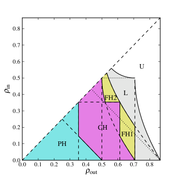
Figure 5: Parameter space of the three-dimensional periodic Lorentz gas as a function of the geometrical parameters $\rho_{\mathrm{out}}$ and $\rho_{\mathrm{in}}$. Solid lines divide regimes of qualitatively different behaviour, which are also shaded with different colours and labelled as follows: PH: planar horizon; CH: cylindrical horizon; FH1 and FH2: finite horizon; L: localised, non-diffusive motion; U: undefined (all space filled). Note that the FH regime is divided into two disjoint regions. The dashed lines mark the different conditions referred to in the text. The diagonal dotted line separates regions where the $\rho_{\mathrm{in}}$-spheres do (above) and do not (below) overlap the $\rho_{\mathrm{out}}$-spheres. The diagram is reflection-symmetric in the line $\rho_{\mathrm{in}}=\rho_{\mathrm{out}}$, but for clarity only the lower half is shown.

Parameter space

The complete parameter space of this model is shown in figure 5, exhibiting the regions in parameter space corresponding to the regimes of qualitatively different behaviour discussed above. Note that if $\rho_{\mathrm{in}}>\sqrt{3}/2-\rho_{\mathrm{out}}$, then the $\rho_{\mathrm{out}}$- and $\rho_{\mathrm{in}}$-spheres overlap, and if $\rho_{\mathrm{in}}>0.5$ then neighbouring $\rho_{\mathrm{in}}$-spheres also overlap. These conditions are marked by the dotted lines in the figure.

4 Persistence in the diffusive regimes of the three-dimensional Lorentz gas

In this section, we study the dependence of the diffusion coefficient on the geometrical parameters of the 3D periodic Lorentz gas model in the finite- (FH1) and cylindrical-horizon (CH) regimes, comparing the numerical results with the finite-memory approximations (2.8), (2.32) and (2.44).

4.1 Approximation by the NMA process

The computation of the dimensional formula (2.8) relies on that of the residence time $\tau$. An exact formula is available for this quantity [27]:

$$\tau=\frac{|Q|}{|\partial Q|}\frac{|S^{2}|}{|B^{2}|},$$ (4.1)

where $|Q|$ denotes the volume of the billiard domain outside the obstacles, $|\partial Q|$ the surface area of the available gaps separating neighbouring cells, $|S^{2}|=4\pi$ the surface area of the unit sphere in three dimensions, and $|B^{2}|=\pi$ the volume (area) of the unit disk in two dimensions, and we assume unit velocity. The explicit formulas giving the values of $|Q|$ and $|\partial Q|$ are rather lengthy and will not be given here; see reference [28].

The validity of equation (4.1) can be tested by comparison with numerical computation of the residence time, as shown in figure 6. Here, and in the remainder of the paper, we restrict attention to values of $\rho_{\mathrm{out}}$ close to the limiting value $1/\sqrt{2}$ and $\rho_{\mathrm{in}}$ close to $0$, so that the geometry is that of a single, cubic unit cell.

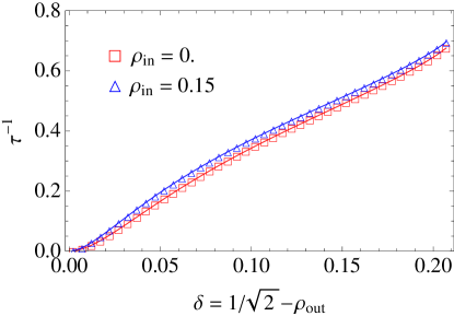
Figure 6: Residence time $\tau$, equation (4.1), compared to direct numerical simulations. The results are shown for two values of the inner radius, $\rho_{\mathrm{in}}=0$ and $\rho_{\mathrm{in}}=0.15$, as functions of $\delta\equiv 1/\sqrt{2}-\rho_{\mathrm{out}}$, which is the characteristic size of the gaps separating neighbouring cells. The curves are very similar since the volume of the inner sphere remains small. In this and the following results we take $\ell=1$.

4.2 Approximation by the 1SMA and 2SMA processes

Single- and two-step memory processes can be derived as approximations, at the lattice level, to the dynamics of the Lorentz gas. This is done by computing numerically the statistics of tracer particles as they jump from cell to cell, so as to estimate the single- and two-step memory probability transitions.

The results are shown in figure 7 for the single-step memory process, where the six transition probabilities $P_{i}$, $i=0,\ldots,5$, are displayed as functions of the outer radius $\rho_{\mathrm{out}}$ for different values of the inner radius $\rho_{\mathrm{in}}$.

For the two-step process, the computation of the transition probabilities $P_{i,j}$ is shown in figure 8 for $\rho_{\mathrm{in}}=0$, that is in the absence of a sphere at the center of the cell. The six different panels each correspond to a given $i=0,\ldots,5$. The same is shown in figure 9 for $\rho_{\mathrm{in}}=0.15$.

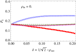
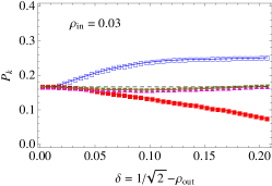
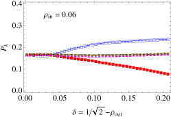
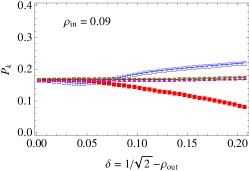
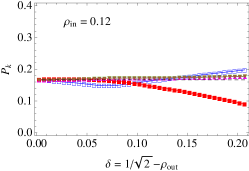
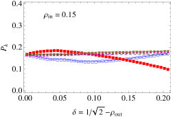
Figure 7: Numerical computations of the probabilities $P_{0},\ldots,P_{5}$ of the single step memory process, appearing in (2.13). The six panels shown correspond to as many different values of $\rho_{\mathrm{in}}$, where the probabilities are shown as functions of $\delta$. The dashed line at $P_{k}=1/6$ indicates the value for a memoryless (NMA) walk. Here and in figures 8 and 9, the conventions are as follows: Empty squares (blue), $P_{0}$; empty upward triangles (cyan), $P_{1}$; empty downward triangles (green), $P_{2}$; filled squares (red) $P_{3}$; filled upward triangles (magenta), $P_{4}$; filled downward triangles (brown), $P_{5}$. In all cases we verify the symmetry $P_{1}=P_{2}=P_{4}=P_{5}$, which also remain close to $1/6$.

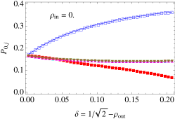
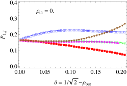
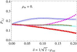
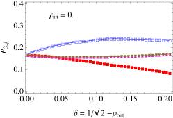
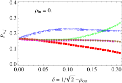
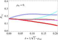
Figure 8: Numerical computations of the 36 probabilities $P_{i,j}$ which appear in (2.36), corresponding to a cell with no sphere at its center, i.e. the inner radius $\rho_{\mathrm{in}}=0$. The symmetries of the process are reflected by the similarities between figures 8, 8, 8 and 8. The colour coding is similar to figure 7.

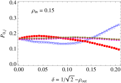
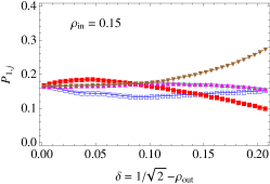
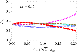
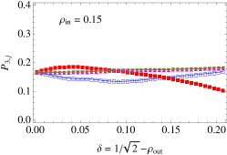
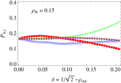
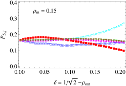
Figure 9: Numerical computations of the probabilities 36 $P_{i,j}$ which appear in (2.36), corresponding to inner radius $\rho_{\mathrm{in}}=0.15$. Here again the symmetries of the process are reflected by the similarities between figures 9, 9, 9 and 9.

4.3 Diffusion coefficient of the billiard

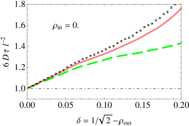
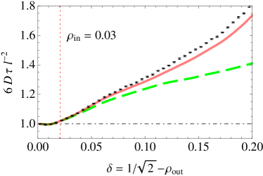
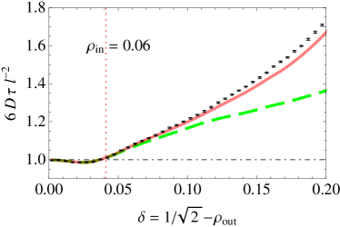
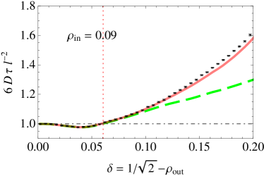
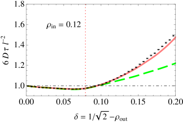
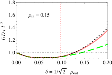
Figure 10: Diffusion coefficient normalised with respect to the dimensional prediction $D_{\mathrm{NMA}}$, equation (2.8), vs. gap size $\delta=1/\sqrt{2}-\rho_{\mathrm{out}}$, plotted for different values of the inner radius $\rho_{\mathrm{in}}=0,\ldots,0.15$. The symbols (black) correspond to direct numerical computation of this quantity, the long dashed (green) lines to the single-step memory diffusion coefficient (2.32), and the solid (red) lines to the two-step memory diffusion coefficient (2.44). The vertical dotted lines indicate the separation between the finite and infinite horizon regimes.

Having computed the probability transitions associated to the single and two-step memory processes, we can compute the invariant distribution $\mathsf{P}$ and substitute the results into equations (2.32) and (2.44) to obtain values of the diffusion coefficients. These are compared to the diffusion coefficient of the billiard calculated from direct simulations in figure 10.

We can draw several conclusions from the results shown in figure 10. Firstly, we remark that in the 3D model studied here there is relatively little back-scattering, i.e. motion in which the particle reverses its direction between arriving and leaving a given cell. This gives an important contribution to the diffusion coefficient, and, in particular, corresponds to the fact that here we find that the diffusion coefficient is larger than the memoryless (NMA) approximation, while in reference [12] the diffusion coefficient tended to lie below the results of this approximation. Note, however, that this effect depends strongly on the particular model used.

It is also interesting to note that in the finite-horizon regime, i.e. left of the dotted vertical lines in figures 10-10, approximating the diffusion coefficient by the one-step memory process (2.32) is just as good as the two-step process (2.44). In the cylindrical-horizon regime, however, the two results are different; the single-step approximation gets poorer as $\rho_{\mathrm{out}}$ decreases, whereas the two-step process yields more accurate estimates. This corresponds to the fact that correlations decay more slowly in the cylindrical-horizon regime [19], so that memory effects persist for longer.

5 Conclusions

The cyclic structures of certain regular lattices underly symmetries of their statistical properties which can be exploited to greatly simplify their analysis. Examples are two-dimensional lattices such as the square, the honeycomb and the triangular lattice, which were studied in reference [2]. Other examples include, in higher dimensions, the hypercubic lattices studied in this paper. Having exhibited the cyclic structures of these lattices, we were able to extend our previous results to hypercubic lattices with suitable adaptations, in order to calculate the diffusion coefficients of persistent random walks with up to two steps of memory.

Our method is especially useful to compute the correlations of persistent walks on such regular lattices. In particular, the velocity autocorrelations of a two-step persistent walk may be recast in terms of matrix powers, which can then easily be resummed to obtain a readily-computable expression for the diffusion coefficient.

Among the many applications of persistent random walks, deterministic diffusive processes are ideal candidates to apply our method. The three-dimensional periodic Lorentz gas is particularly interesting as it exhibits two distinct types of diffusive regimes, one with finite horizon, where memory effects decay fast, and another with cylindrical horizon, where memory effects can remain important. In this latter case, the approximation of the diffusive process by a two-step memory walk proves much more accurate than the single-step process.

We remark that the application of our formalism to the diffusive properties of Lorentz gases relies on the numerical computation of the transition probabilities corresponding to the persistent process with which we approximate the deterministic process. Since there are $30$ transition probabilities for the two-step memory walk, their analytical calculation is a daunting task. It relies on knowledge of the statistics of trapped trajectories and involves contributions from different time scales. Nonetheless, this computation is formally possible, and is in principle much simpler than that of the actual diffusion coefficient.

References

References

- [1] Haus J W and Kehr K W 1987 Diffusion in regular and disordered lattices Phys. Rep. 150 263.
- [2] Gilbert T and Sanders D P 2010 Diffusion coefficients for multi-step persistent random walks on lattices J. Phys. A Math. Theor. 43 5001.
- [3] Geisel T and Nierwetberg J 1982 Onset of diffusion and universal scaling in chaotic systems Phys. Rev. Lett. 48 7.
- [4] Fujisaka H and Grossmann S 1982 Chaos-induced diffusion in nonlinear discrete dynamics Z. Phys. B 48 261.
- [5] Schell M, Fraser S and Kapral R 1983 Subharmonic bifurcation in the sine map: An infinite hierarchy of cusp bistabilities Phys. Rev. A 28 373.
- [6] Grassberger P 1983 New mechanism for deterministic diffusion Phys. Rev. A 28 3666.
- [7] Gaspard P 1998 Chaos, Scattering and Statistical Mechanics (Cambridge: Cambridge University Press).
- [8] Cvitanović P and Artuso R 2010 Chapter “Deterministic diffusion” in Cvitanović P, Artuso R, Mainieri R, Tanner G, and Vattay G Chaos: Classical and Quantum ChaosBook.org/version13 (Copenhagen: Niels Bohr Institute)
- [9] Dorfman J R 1999 An Introduction to Chaos in Nonequilibrium Statistical Mechanics (Cambridge: Cambridge University Press).
- [10] Klages R and Dorfman J R 1995 Simple maps with fractal diffusion coefficients Phys. Rev. Lett. 74 387.
- [11] Klages R and Dorfman J R 1999 Simple deterministic dynamical systems with fractal diffusion coefficients Phys. Rev. E 59 5361.
- [12] Gilbert T and Sanders D P 2009 Persistence effects in deterministic diffusion Phys. Rev. E, 80 41121.
- [13] Bunimovich L A and Sinai Ya G 1980 Markov partitions for dispersed billiards Commun. Math. Phys. 78 247.
- [14] Bunimovich L A and Sinai Ya G 1981 Statistical properties of Lorentz gas with periodic configuration of scatterers Commun. Math. Phys. 78 479.
- [15] Zacherl A, Geisel T, Nierwetberg J, and Radons G 1986 Power spectra for anomalous diffusion in the extended Sinai billiard Phys. Lett. A 114 317.
- [16] Bleher P M 1992 Statistical properties of two-dimensional periodic Lorentz gas with infinite horizon J. Stat. Phys. 66 315.
- [17] Szasz D and Varjú T 2007 Limit laws and recurrence for the planar Lorentz process with infinite horizon J. Stat. Phys. 129 59 2007.
- [18] Chernov N 1994 Statistical properties of the periodic Lorentz gas. Multidimensional case J. Stat. Phys. 74 11.
- [19] Sanders D P 2008 Normal diffusion in crystal structures and higher-dimensional billiard models with gaps Phys. Rev. E 78 060101.
- [20] Machta J and Zwanzig R 1983 Diffusion in a periodic Lorentz gas Phys. Rev. Lett. 50 1959.
- [21] Klages R and Dellago C 2000 Density-dependent diffusion in the periodic Lorentz gas J. Stat. Phys. 101 145.
- [22] Klages R and Korabel N 2002 Understanding deterministic diffusion by correlated random walks J. Phys. A Math. Gen. 35 4823.
- [23] Klages R 2007 Microscopic Chaos, Fractals and Transport in Nonequilibrium Statistical Mechanics (Singapore: World Scientific).
- [24] Sanders D P 2008 Deterministic Diffusion in Periodic Billiard Models (PhD thesis, University of Warwick, 2005) arXiv preprint arXiv:0808.2252.
- [25] Henk M and Zong C 2000 Segments in ball packings Mathematika, 47 31.
- [26] Garrido P L 1997 Kolmogorov–Sinai entropy, Lyapunov exponents, and mean free time in billiard systems J. Stat. Phys. 88 807.
- [27] Chernov N 1997 Entropy, Lyapunov exponents, and mean free path for billiards J. Stat. Phys., 88 1.
- [28] Nguyen H C 2010 Etude du comportement diffusif d’un billard chaotique à trois dimensions et son approximation par une marche aléatoire persistante Thèse de Master, Université Libre de Bruxelles.