Truncation errors in self-similar continuous unitary transformations

Abstract

Effects of truncation in self-similar continuous unitary transformations (S-CUT) are estimated rigorously. We find a formal description via an inhomogeneous flow equation. In this way, we are able to quantify truncation errors within the framework of the S-CUT and obtain rigorous error bounds for the ground state energy and the highest excited level. These bounds can be lowered exploiting symmetries of the Hamiltonian. We illustrate our approach with results for a toy model of two interacting hard-core bosons and the dimerized $S=\nicefrac{{1}}{{2}}$ Heisenberg chain.

In 1994, Wegner Wegner (1994) introduced the method of continuous unitary transformations (CUT) to many-body physics. Independently, a similar method was developed by Głazek and Wilson denoted as similarity renormalization scheme Głazek and Wilson (1993, 1994) to be used in QED and QCD. In this non-perturbative approach, a Hamiltonian is mapped to an effective, renormalized model by a series of infinitesimal unitary transformations specified by the flow equation. This effective Hamiltonian shows (block-)diagonal structure and can be used to calculate ground state and low-energy properties as well as observables Kehrein and Mielke (1997, 1998). A perturbative variant (P-CUT) allows for systematic high-order perturbation expansions Uhrig and Normand (1998); Knetter and Uhrig (2000); Knetter (2003). Additionally, the CUT method provides a generic framework to derive effective models for many-particle systems that incorporate the relevant physics. The mapping of the Hubbard model to a generalized $t$-$J$ model illustrates this point exemplarily Reischl et al. (2004); Reischl (2006); Lorscheid (2007); Hamerla (2009); Hamerla et al. (2010).

Techniques based on CUT have been applied successfully in various fields of many-particle physics as electron-phonon-coupling Lenz and Wegner (1996); Mielke (1997), spin-chains Schmidt and Uhrig (2003); Schmidt (2004) and ladders Schmidt and Uhrig (2005); Fischer et al. (2010), anyonic excitations Schmidt et al. (2008); Dusuel et al. (2008); Vidal et al. (2008) or non-equilibrium problems Kehrein and Mielke (1997) to mention only a few. For an overview, see Refs. Wegner, 2006 and Kehrein, 2006.

The basic concept of CUT is to transform the problem of (block-)diagonalising a Hamiltonian into to the solution of a differential equation for the Hamiltonian

$$\partial_{\ell}H(\ell)=\left[\eta(\ell),H(\ell)\right],$$ (1)

commonly known as flow equation . The initial Hamiltonian $H(0)$ is linked continuously to a unitarily equivalent (block-)diagonal or otherwise simpler Hamiltonian $H(\infty)$ in the limit of infinite $\ell$.

A drawback of the CUT method is the creation of more complex interaction in the Hamiltonian during the flow. To keep the set of equations finite, it is necessary to define a truncation scheme and thereby keep only a finite number of multi-particle interactions. These truncation errors result in unknown errors for the calculated physical quantities. A common approach is to start with a strict truncation scheme, i.e., a scheme comprises only a limited number of terms in the Hamiltonian, and to justify this scheme a posteriori by comparing it to calculations using less strict truncation schemes Kehrein and Mielke (1994). This yields a pragmatically well-working method to control the quality of the calculated quantities. However, since this approach only compares different approximations, the relation to the exact result or rigorous error bounds are out of reach.

In our work, we analyze the effects of truncation to the flow and show how the truncation can be treated in a mathematical framework. Thereby, we aim to quantify the truncation error a priori. This approach will lead to rigorous bounds for the ground state energy and the highest energy eigen-value for the Hamiltonian.

The paper is structured as follows: After this introduction, we give an overview of the CUT method. In Sect. II, we analyze the truncation and define the truncation error. The formalism developed is applied to the double hard-core boson model in Sect. III to provide a transparent, simple application. Subsequently, we discuss in Sect. IV the modifications needed for the calculation of truncation errors in extended systems. For further illustration, we show results for the dimerized Heisenberg chain. Finally, a summary is given.

I The CUT method

I.1 Homogeneous flow equation

Probably, unitary transformations are one of the most widely used techniques in studies on Hamiltonians. They render a description of a Hamiltonian possible in a more appropriate basis in which the physical properties can be studied more easily. Most desirably, every Hamiltonian can be diagonalized by a certain unitary transformation. Unfortunately, this transformation is usually unknown.

The basic idea of the CUT-method is not to search for such a transformation in one step, but to bring the Hamiltonian successively closer to a simpler shape by a series of infinitesimal transformation. Therefore, a continuous flow parameter $\ell$ is introduced that parametrizes the continuous unitary transformation $U(\ell)$. The Hamiltonian is considered to become a function $H(\ell)=U(\ell)H^{(b)}U^{\dagger}(\ell)$ of this parameter. In this way, the initial (bare) Hamiltonian $H^{(b)}$ is linked continuously by a unitary transformation to the renormalized Hamiltonian showing the intended structure $H^{(r)}=H(\infty)$ in the limit of infinite $\ell$. By derivation with respect to $\ell$, one obtains the flow equation

$$\partial_{\ell}H(\ell)= \frac{\partial U(\ell)}{\partial\ell}U^{\dagger}(\ell)H(\ell)+H(\ell)U(\ell)\frac{\partial U^{\dagger}(\ell)}{\partial\ell}$$ (2a)

$$= \left[\eta(\ell),H(\ell)\right].$$ (2b)

The antihermitian generator $\eta$ of the transformation reads

$$\eta(\ell)=\frac{\partial U(\ell)}{\partial\ell}U^{\dagger}(\ell)=-\eta^{\dagger}(\ell).$$ (3)

Equation (2) is linear differential equation for the Hamiltonian. We emphasize that also all intermediate Hamiltonians $H(\ell)$ conserve the full information of the system because they are only written in a different basis.

Since the basis has changed during the flow, observables may not be calculated directly using their bare operator $\mathcal{O}^{(b)}$ but have also to be transformed by a similar flow equation

$$\partial_{\ell}\mathcal{O}(\ell)=\left[\eta(\ell),\mathcal{O}(\ell)\right].$$ (4)

The transformation of observables was used first by Kehrein and Mielke to determine correlation functions for dissipative bosonic systems Kehrein and Mielke (1997, 1998).

I.2 Generator schemes

Up to here, the problem of diagonalization has only been recast in the form of determining an appropriate generator $\eta(\ell)$. The key ingredient of the CUT-method is to choose the generator as manifestly antihermitian operator depending on the flowing Hamiltonian. We denote the superoperator $\hat{\eta}:H(\ell)\to\eta(\ell)=\hat{\eta}[H(\ell)]$ as generator scheme to distinguish between the mapping $\hat{\eta}$ and the function $\eta(\ell)$. In this way, the flow equation for the Hamiltonian (2) becomes non-linear, while the transformation of observables (4) stays linear. The generator scheme has to be designed in a way that the flow equation has attractive fixed points where the Hamiltonian has the desired structure. In this manner, (block-)diagonality can be obtained by merely integrating the flow equation Wegner (1994); Mielke (1998); Knetter and Uhrig (2000); Dusuel and Uhrig (2004).

For the first generator scheme introduced by Wegner Wegner (1994), the Hamiltonian $H(\ell)=H_{\text{d}}(\ell)+H_{\text{nd}}(\ell)$ has to be decomposed into a diagonal $H_{\text{d}}$ and a non-diagonal part $H_{\text{nd}}$. The generator is defined as a commutator

$$\eta(\ell)=\widehat{\eta}_{\text{W}}[H(\ell)]=\left[H(\ell),H_{\text{nd}}(\ell)\right]=\left[H_{\text{d}}(\ell),H_{\text{nd}}(\ell)\right]$$ (5)

of the diagonal and non-diagonal-part of the Hamiltonian. One directly realizes that a vanishing non-diagonality yields a fixed point of the flow. The proof of convergence for unapproximated systems was given by Wegner Wegner (1994) for finite matrices and extended to infinite systems by Dusuel and Uhrig Dusuel and Uhrig (2004). The generator decouples eigen-subspaces of different energy eigen-values, but it is not able to treat degeneracies. In his original work concerning the $n$-orbital model Wegner (1994), Wegner noticed divergences. He could avoid them via taking only terms violating the number of quasiparticles into account in the definition of $H_{\text{nd}}$ aiming at block-diagonality instead of diagonality. In this manner, the complexity of the a problem can still be reduced significantly because different quasiparticle spaces can be studied separately.

To overcome the problem of residual off-diagonality due to degeneracies, Mielke Mielke (1998) introduced a generator scheme on the matrix level based on a sign function of index differences $\eta_{ij}=\text{sign}(i-j)h_{ij}$ that always yields a diagonal Hamiltonian. Independently, Knetter and Uhrig Uhrig and Normand (1998); Knetter and Uhrig (2000) developed a similar scheme which concentrates more generally on a quasiparticle picture. In their approach, the Hamiltonian $H(\ell)=\sum_{ij}H^{i}_{j}(\ell)$ is decomposed into different blocks $H^{i}_{j}$ of terms with respect to the number $i$ of quasiparticles created and the number $j$ of quasiparticles annihilated by the term. In this notation, the generator scheme acts as

$$\widehat{\eta}_{\text{pc}}[H(\ell)]=\sum\limits_{i,j}\text{sgn}\left(i-j\right)H^{i}_{j}(\ell).$$ (6)

In the limit of infinite $\ell$, the Hamiltonian converges to a block-diagonal, quasiparticle conserving structure if the spectrum is bounded from below Mielke (1998); Knetter and Uhrig (2000); Dusuel and Uhrig (2004). Blocks with $i\neq j$ decay exponentially with rising $\ell$. During the flow, the quasiparticle spaces are ordered ascending to their energy eigen-valueMielke (1998); Heidbrink and Uhrig (2002). This implies that the vacuum state, i.e., the state with $j=0$, is mapped to the ground state of the Hamiltonian if it is not degenerated.

A special feature of this generator scheme is that it strictly conserves the block-band structure of the Hamiltonian during the flow. A similar generator was used by Stein Stein (1997, 1998) in a case where the sign function was not necessary. In contrast to Wegner’s generator scheme, the right-hand side of the flow equation for the Hamiltonian (2) is only quadratic in the Hamiltonian’s coefficients instead of cubic.

A recent development in the field of generator schemes is the ground state generator Fischer et al. (2010)

$$\widehat{\eta}_{\text{gs}}[H(\ell)]=H^{i}_{0}(\ell)-H^{0}_{j}(\ell).$$ (7)

The definition resembles the particle conserving scheme, but it is designed to decouple only the zero quasiparticle subspace of a system, i.e., the ground state if not degenerated. It was introduced by Fischer, Duffe, and Uhrig to describe quasiparticles decays, since the picture of conserved renormalized quasiparticles becomes very cumbersome.

Compared to the particle conserving scheme, $\widehat{\eta}_{\text{gs}}$ exhibits an enhanced numerical stability and saves computational ressources due to its fast convergence. As a drawback, it does not conserve the block-band structure as $\widehat{\eta}_{\text{pc}}$ does. In this work, we will make use of both generator schemes, $\widehat{\eta}_{\text{pc}}$ and $\widehat{\eta}_{\text{gs}}$.

I.3 Truncation scheme

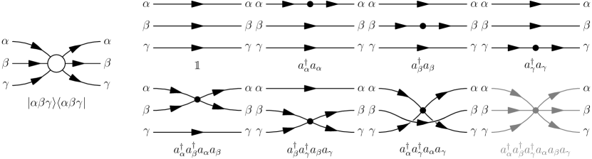
Figure 1: Decomposition of the diagonal element for the three-particle state $\left|\alpha\beta\gamma\right\rangle$ into irreducible interaction processes. By truncation of three-particle processes, only the three-particle irreducible term $a^{\dagger}_{\alpha}a^{\dagger}_{\beta}a^{\dagger}_{\gamma}a_{\alpha}a_{\beta}a_{\gamma}$ is neglected.

One way to solve the flow equation (2) is to parameterize the Hamiltonian in second quantization by an adequate operator basis. In this way, the differential equations for the coefficients of the operators are found by computing the commutator on the right hand side in (2) and re-expressing the result again in the operator basis chosen. The evaluation of the commutator generates new many-body interaction processes that are not present in the initial Hamiltonian. They have to be incorporated in the Hamiltonian which results in an iterative calculation of the commutator. This proliferation of terms generically yields an infinite number of differential equations which is intractible in practical applications. Four different strategies have evolved to obtain a closed the set of differential equations:

On restricting to finite systems, the flow equation can be solved exactly both on the level of second quantization or on the level of matrix elements. As a drawback, this approach is subjected to the same limitation as other finite-size methods. Furthermore, the differential equation system may still be large enough to require further approximations for practical applications.

In some special cases, it is possible to obtain a closed system of equations by identifying a small expansion parameter. In his original work Wegner (1994), Wegner investigated the $n$-orbital model. He was able to close the system of differential equations in the limit of infinite $n$. However, these advantageous cases do not show up in every system or are simply out of interest. In general, approximations have to be applied to the system to overcome the problem of proliferation of terms.

In the method of perturbative continuous unitary transformations (P-CUT) introduced by Knetter and Uhrig Uhrig and Normand (1998); Knetter and Uhrig (2000); Knetter (2003), the non-diagonality $H_{\text{nd}}$ is considered as small perturbation to the diagonal part $H_{\text{d}}$ of the bare Hamiltonian. In this way, the flow equation can be expanded and therefore used to apply perturbation theory up to very high orders.

The non-perturbative approach, which we will use in this work, is dubbed self-similar continuous unitary transformations (S-CUT). Here a truncation scheme is defined that incorporates all terms considered to be important to the problem while other terms are neglected. In view of the numerous degrees of freedom, the choice of an adequate truncation scheme is a non-trivial task. It has to respect the system’s physical properties. Since the structure of the Hamiltonian does not change during the flow, it is named self-similar. As a rule of thumb, a calculation is considered to be the more reliable the more terms are included in the truncation scheme. Due to truncation, the modified flow equation reads

$$\partial_{\ell}H(\ell)=\widehat{T}\left[\eta(\ell),H(\ell)\right].$$ (8)

Here we introduced the superoperator $\widehat{T}$ which denotes the application of the truncation scheme.

A natural description for many-body problems is provided by second quantization. Since most of the low-energy physics can be preserved by low numbers of suitable quasiparticles, it is useful to define a truncation scheme neglecting all terms that create or annihilate more than a given number of quasiparticles. We emphasise that this truncation expressed second quantization does not imply any restriction of the Hilbert space which is to be considered a major advantage.

We stress that the action of a Hamiltonian on a state containing $n$ quasiparticles can be split into a sum of irreducible terms affecting at most $m\leq n$ quasiparticles each (see Fig. 1). Thus, the truncation of high-particle irreducible processes does not imply the complete neglect of matrix elements between states of high quasiparticle numbers, but rather an extrapolation based on lower quasiparticle irreducible processes.

In extended systems, often additional truncation criteria have to be applied in order to close the set of differential equations. An obvious choice for gapped systems with finite correlation lengt is to truncate according to the real-space range of the physical process generated by the term under study. We make use of this real-space truncation in Sect. IV.

Truncations cause quantitative errors in the calculated physical quantities and may possibly lead to divergences of the truncated flow, even though convergence has been proven for the untruncated flow. In their analysis of the flow equations for the Anderson model Kehrein and Mielke (1994), Kehrein and Mielke used a strict truncation scheme that includes only contributions of types that are already present in the bare Hamiltonian.

In a second step, they included a new contribution to the scheme and analyzed the new equations in order to assess its relevance. In their classification, terms that affect other matrix elements only by quantitative deviations and vanish in the limit $\ell\to\infty$ are denoted as irrelevant, or as marginal if they converge to a finite value. Only terms that are able to change the behavior of the flow equations qualitatively, for instance that cause divergences if they are not treated properly, were considered to be relevant. This approach is suited to ensure the correct qualitative behavior of the effective model derived from the CUT. But it does not provide a quantitative measure of the truncation errors.

I.4 Symmetries

For practical computations, exploiting symmetries of the Hamiltonian is generally very useful. To study Hamiltonians of systems with an infinite number of sites, the use of translation symmetry is inevitable. Let us suppose that we have chosen a basis of operators to express the Hamiltonian. Each term in the Hamiltonian is given by one of these basis operators multiplied by a prefactor, its coefficient.

Although the Hamiltonian is symmetric under a group of specific symmetry transformations, the symmetry of each individual basis operator may be lower. In this case, the coefficients of several basis operators fulfil linear conditions to ensure that their combination is invariant under the symmetry group. By parametrizing the Hamiltonian in terms of linearly independent symmetric combinations of basis operators, the number of coefficients to be tracked is significantly reduced saving both computation time and memory. Technically this can be done by selecting one operator as a unique representative from which the complete symmetric combination can be obtained by taking the sum $\sum_{G}$ over a specific subgroup of the symmetry group of the Hamiltonian.

We emphasize that in general one has to clearly distinguish between the symmetry group of the Hamiltonian and the superoperator $\sum_{G}$. Even if the Hamiltonian displays a continuous symmetry such as the $\text{SU}(n)$ spin rotation symmetry, the number of constraints that can be derived for the coefficients of the Hamiltonian’s terms is limited. Excluding translation symmetries, this means that only a finite number of terms are represented by one representative operator. Therefore the number of symmetry operations to build the symmetric combination from a single representative is often finite although the exploited symmetry is continuous. In summary, we take the superoperation $\sum_{G}$ as a technical tool to benefit from the Hamiltonian’s underlying full symmetry group.

Moreover, the precise meaning of $\sum_{G}$ depends on the representative under study. As an example, a representative that shares the whole symmetry of the Hamiltonian, e.g., unity, is already identical to its corresponding symmetric combination. To this operator, $\sum_{G}$ acts as identity. The other limit is a representative operator that does not share any of the Hamiltonian’s symmetries. The superoperator $\sum_{G}$ applied to such a representative has to generate the fully symmetric combination of basis operators.

Since the sums $\sum_{G}$ occur on both sides of Eq. (2), the modified flow equation can be reduced to a representative expression requiring a sum for only one argument of the commutator. Correction factors have to be introduced since different representative basis operators appearing in the commutator give rise to different numbers of basis operators in the fully symmetric combination which they represent. Details on the implementation of symmetries in S-CUT can be found in Ref. Reischl, 2006.

II Mathematical analysis of truncation errors

II.1 Effects of truncation

On truncating the flow equation, all information about the truncated terms is lost. It is common practice to neglect terms which are considered to be unimportant and to justify this a posteriori. But even if these terms are not subject of the intended analysis of the effective Hamiltonian, their omission leads to quantitative deviations for the coefficients of all terms in the Hamiltonian because they are linked by the differential equations. We stress that the commutator of the generator and a truncated term may result in terms that comply with the truncation scheme, i.e., that we want to compute quantitatively. Thus the loss of information cannot be limited to certain terms only. Generically, truncation introduces errors in all coefficients of the Hamiltonian.

Because of truncation, the transformation of a Hamiltonian $H(\ell)$ described by the truncated flow equation (8) does not need to be unitary anymore. Therefore, the spectrum of $H(\ell)$ will be distorted during the flow. Physical quantities calculated based on the effective Hamiltonian are affected by finite inaccuracies. In the following sections II.2-E, we present a formalism to bound these errors rigorously.

An additional physical consequence of truncation can be derived for real-space truncation schemes which neglect interactions beyond a certain range $d>d_{\text{max}}$ (see Sect. I.3). Due to the formulation in second quantization, the S-CUT method is capable to handle infinite systems. Nevertheless, the truncation by range affects correlations on larger length scales. We observed that the coefficients of representatives in a truncated infinite system and a truncated periodic system with a certain size $l\geq L_{\text{fin}}$ share the same set of differential equations, if the algebra is local. Any possibility to observe that the system size is actually finite is masked by the truncation scheme if the system size is at least $L_{\text{fin}}=3d_{\text{max}}+1$.

Therefore also the intensive physical properties of an infinite system determined using S-CUT with truncation range $d_{\text{max}}$ are identical to those of a finite system with a certain size $l\geq L_{\text{fin}}$ and periodic boundary conditions. The quantity $L_{\text{fin}}$ can be understood as an effective size introduced by the real-space truncation scheme. The mathematical derivation including a numerical verification is given in Appendix A.

II.2 Splitting the flow equation

To isolate the truncation error of S-CUT, we start from the full flow equation

$$\partial_{\ell}H(\ell)=[\eta^{\prime}(\ell),H(\ell)]$$ (9)

for the unitarily transformed Hamiltonian $H(\ell)$ with $H(\ell=0)=H^{(\text{b})}$. The generator $\eta^{\prime}$ appears instead of $\eta$ because in practice the generator is determined from the truncated Hamiltonian $H^{\prime}$ and not from $H$, see Eq. (12).

We decompose $H$ into two parts: the solution $H^{\prime}$ from a truncated flow equation and the difference $H^{\prime\prime}=H-H^{\prime}$ between the truncated and the non-truncated calculation. Next, the flow equation (9) can be split into the system

$$\partial_{\ell}H^{\prime}(\ell) = \widehat{T} [\eta^{\prime}(\ell),H^{\prime}(\ell)]$$ (10a)

$$\partial_{\ell}H^{\prime\prime}(\ell) = (\mathbbm{1}-\widehat{T}) [\eta^{\prime}(\ell),H^{\prime}(\ell)]+[\eta^{\prime}(\ell),H^{\prime\prime}(\ell)]$$ (10b)

of differential equations for $H^{\prime}$ and $H^{\prime\prime}$. As initial conditions, we choose

$$H^{\prime}(0)\ = \ H^{(\text{b})}$$ (11a)

$$H^{\prime\prime}(0)\ = \ 0.$$ (11b)

Obviously, the sum of the equations (10) with the initial condition (11) reproduce the flow equation (9) with its initial condition.

Up to now, the generator $\eta^{\prime}$ is not specified. Using the generator scheme $\widehat{\eta}$, we define the generator

$$\eta^{\prime}(\ell)=\widehat{\eta}[H^{\prime}(\ell)]$$ (12)

as a function of the truncated Hamiltonian. Note that this choice does not violate the unitarity of the transformation because the generator $\eta^{\prime}$ continues to be manifestly antihermitian.

Equation (10a) provides a closed set of differential equations for the coefficients of the truncated Hamiltonian which can be treated by numerical integration. This leads to an effective Hamiltonian $H^{\prime}(\infty)=H^{\prime(\text{r})}$ with a structure determined by the chosen generator scheme.

In contrast, the full Hamiltonian $H$ is transformed by a true unitary transformation, but does not need to have any special structure in the limit of infinite $\ell$, since it is transformed like an observable by $\eta^{\prime}$. However, it is to be expected that it is close to $H^{\prime}$ if truncation errors are small.

The difference $H^{\prime\prime}$ stores the complete ‘non-unitarity‘ of the transformation of $H^{\prime}(\ell)$. Mathematically, Eq. (10b) describes a transformation of $H^{\prime\prime}$ via a flow equation with an additional inhomogeneity

$$\kappa(\ell)=(\mathbbm{1}-\widehat{T}) [\eta^{\prime}(\ell),H^{\prime}(\ell)]$$ (13)

depending on $H^{\prime}(\ell)$. This natural emergence of an inhomogeneous flow equation is quite remarkable and has not been observed before to our knowledge. We emphasise that the number of equations defining $\kappa(\ell)$ remains finite if $H^{\prime}$ and thus $\eta^{\prime}$ are restricted by the truncation scheme to a finite number of terms. Hence the computation of $\kappa(\ell)$ is indeed feasible. Of course, this is not true for $H^{\prime\prime}$.

II.3 Inhomogeneous flow equation

To solve the inhomogeneous flow equation (10b), we use the ansatz

$$H^{\prime\prime}(\ell)=U(\ell)A(\ell)U^{\dagger}(\ell)$$ (14)

with $A(0)=H^{\prime\prime}(0)=0$. The unitary transformation $U(\ell)$ is linked to the generator $\eta^{\prime}(\ell)$ of the transformation by Eq. (3). The formal solution for $U(\ell)$ using the $\ell$-ordering operator $\mathcal{L}$ reads

$$U(\ell)=\mathcal{L}\exp\left(\int\limits_{0}^{\ell}\eta^{\prime}(\ell^{\prime})\mathsf{d}\ell^{\prime}\right).$$ (15)

Using variation of parameters

$$\partial_{\ell}H^{\prime\prime}(\ell) =\left[\eta^{\prime}(\ell),H^{\prime\prime}(\ell)\right]+U(\ell)\partial_{\ell}A(\ell)U^{\dagger}(\ell)$$ (16a)

$$\overset{!}{=}\left[\eta^{\prime}(\ell),H^{\prime\prime}(\ell)\right]+\kappa(\ell),$$ (16b)

leads to the equation

$$A(\ell)=A(0)+\int\limits_{0}^{\ell}U^{\dagger}(\ell^{\prime})\kappa(\ell^{\prime})U(\ell^{\prime})\mathsf{d}\ell^{\prime}.$$ (17)

Therefore, the formal solution of the inhomogeneous flow equation (10b) is given by

$$H^{\prime\prime}(\ell)=U(\ell)\left(H^{\prime\prime}(0)+\int\limits_{0}^{\ell}U^{\dagger}(\ell^{\prime})\kappa(\ell^{\prime})U(\ell^{\prime})\mathsf{d}\ell^{\prime}\right)U^{\dagger}(\ell).$$ (18)

This expression (18) has a very direct interpretation: All contributions of the inhomogeneity up to the given value of $\ell$ are re-transformed to $\ell=0$ and summed. This sum is evaluated after a unitary transformation to the considered flow parameter.

II.4 Truncation error

The formal solution (18) enables the calculation of the distortion of unitarity by the truncated calculation. All effects of the truncation are stored in $H^{\prime\prime}(\ell)$. Certainly, a direct calculation is neither practical nor desirable, because it is equivalent to an untruncated calculation. But for the derviation of a bound of the truncation error only a small part of the information is essential. To assess the quality of the truncation, we are interested in the norm of $H^{\prime\prime}(\ell)$. In particular, we want to focus on norms that are unitarily invariant, i.e., invariant under unitary transformations .

We apply the norm to Eq. (18). Due to its unitary invariance, we obtain

$$\left|\left|H^{\prime\prime}(\ell)\right|\right|=\left|\left|\int\limits_{0}^{\ell}U^{\dagger}(\ell^{\prime})\kappa(\ell^{\prime})U(\ell^{\prime})\mathsf{d}\ell^{\prime}\right|\right|.$$ (19)

In addition, we used $H^{\prime\prime}(0)=0$ from Eq. (11b). To avoid the complicated integration of an operator-valued function, we apply the triangle inequality to the Riemann integral arriving at the upper bound

$$\left|\left|H^{\prime\prime}(\ell)\right|\right| \leq\int\limits_{0}^{\ell}\left|\left|U^{\dagger}(\ell^{\prime})\kappa(\ell^{\prime})U(\ell^{\prime})\right|\right|\mathsf{d}\ell^{\prime}$$ (20a)

$$=\int\limits_{0}^{\ell}\left|\left|\kappa(\ell^{\prime})\right|\right|\mathsf{d}\ell^{\prime}=:\Lambda_{H}(\ell),$$ (20b)

where again the unitary invariance was used. We define the derived quantity $\Lambda_{H}(\ell)$ as truncation error of the transformation. By construction, it is an upper bound for the distance between $H^{\prime}$ and $H$ measured by the selected norm. We emphasize that $\Lambda_{H}(\ell)$ is a scalar function which depends only on the norm of the truncated terms as defined in Eq. (13). It starts at zero and increases monotonically with the flow parameter $\ell$.

Because of the finite and constant number of terms complying with the truncation scheme, the number of contributions to the inhomogeneity $\kappa(\ell)$ stays also constant during the flow. The coefficients of the terms in $\kappa(\ell)$ can be calculated as functions of the coefficients of $H^{\prime}(\ell)$ already known by numerical integration. This is the key simplification compared to the practically impossible direct calculation of $H^{\prime\prime}(\ell)$ or $H(\ell)$.

In the above analysis, the necessary ingredients are the flow equation and the truncation scheme. Hence all considerations can also be carried over to the transformation of observables. The truncation error of an observable $\mathcal{O}$ can be estimated analogously by

$$\Lambda_{\mathcal{O}}(\ell):=\int\limits_{0}^{\ell}\left|\left|(\mathbbm{1}-\widehat{T})[\eta^{\prime}(\ell^{\prime}),\mathcal{O}^{\prime}(\ell^{\prime})]\right|\right|\mathsf{d}\ell^{\prime}\geq\left|\left|\mathcal{O}^{\prime\prime}(\ell)\right|\right|$$ (21)

where $\mathcal{O}$ is decomposed in $\mathcal{O}^{\prime}$ and $\mathcal{O}^{\prime\prime}$ in analogy to (11). The generator is defined by the numerically accessible truncated Hamiltonian $H^{\prime}$.

II.5 Rigorous bounds for observables

The truncation error $\Lambda_{\mathcal{O}}$ is a property of the entire transformation of $\mathcal{O}^{\prime}$ that quantifies the loss of accuracy by truncation. It is desirable to have rigorous bounds for the accuracy of physical quantities calculated by truncated CUTs. Indeed, it is possible to obtain such bounds by calculating the truncation error defined by the spectral norm

$$\left|\left|A\right|\right|_{S}:=\sqrt{\max\ \operatorname{EV}\left(A^{\dagger}A\right)}.$$ (22)

For hermitian operators, the spectral norm is identical to the maximum absolute eigen-value.

We denote the lowest eigen-value of $\mathcal{O}^{\prime}$ by $\Omega^{\prime}_{\text{min}}$ and the associate eigen-state by $\left|\psi^{\prime}\right\rangle$. For the untruncated observable $\mathcal{O}$ we use $\Omega_{\text{min}}$ and $\left|\psi\right\rangle$. Since $\mathcal{O}$ is transformed by a unitary transformation, $\Omega_{\text{min}}$ does not change during the flow whereas $\Omega^{\prime}_{\text{min}}$ is changed due to truncation, for illustration see Fig. 2.

The spectral norm of $\mathcal{O}^{\prime\prime}$ fullfills

$$\left|\left|\mathcal{O}^{\prime\prime}(\ell)\right|\right| \geq\left<\ \mathcal{O}^{\prime\prime}(\ell)\ \right>{}_{{\psi^{\prime}(\ell)}}$$ (23a)

$$=\underbrace{\left<\ \mathcal{O}(\ell)\ \right>{}_{\psi^{\prime}(\ell)}}_{\geq\Omega_{\text{min}}}-\underbrace{\left<\ \mathcal{O}^{\prime}(\ell)\ \right>{\psi^{\prime}(\ell)}}_{\Omega_{\text{min}}^{\prime}(\ell)}.$$ (23b)

By condition, $\Omega_{\text{min}}$ is a lower bound for $\left<\ \mathcal{O}(\ell)\ \right>{}_{{\psi^{\prime}(\ell)}}$. It follows

$$\left|\left|\mathcal{O}^{\prime\prime}(\ell)\right|\right|\geq\Omega_{\text{min}}-\Omega_{\text{min}}^{\prime}(\ell)=:\Delta\Omega_{\text{min}}(\ell).$$ (24)

Analogously, one obtains the inequality

$$\left|\left|\mathcal{O}^{\prime\prime}(\ell)\right|\right| \geq-\left<\ \mathcal{O}^{\prime\prime}(\ell)\ \right>{}_{{\psi(\ell)}}$$ (25a)

$$=-\underbrace{\left<\ \mathcal{O}(\ell)\ \right>{}_{\psi(\ell)}}_{\Omega_{\text{min}}}+\underbrace{\left<\ \mathcal{O}^{\prime}(\ell)\ \right>{}_{\psi(\ell)}}_{\geq\Omega_{\text{min}}^{\prime}(\ell)}.$$ (25b)

Since $\Omega_{\text{min}}^{\prime}(\ell)$ is a lower bound for $\left<\ \mathcal{O}^{\prime}(\ell)\ \right>{}_{{\psi(\ell)}}$, we obtain

$$\left|\left|\mathcal{O}^{\prime\prime}(\ell)\right|\right|\geq-\Omega_{\text{min}}+\Omega_{\text{min}}^{\prime}(\ell)=-\Delta\Omega_{\text{min}}(\ell).$$ (26)

In summary, the truncation error

$$\Lambda_{\mathcal{O}}(\ell)\geq\left|\left|\mathcal{O}^{\prime\prime}(\ell)\right|\right|\geq\left|\Delta\Omega_{\text{min}}(\ell)\right|$$ (27)

is an upper bound of the deviation of the minimal eigen-value of the effective operator due to the truncation. Analogously, one can prove that $\Lambda_{\mathcal{O}}$ defines an upper bound for the deviation of the maximal eigen-value $\Delta\Omega_{\text{max}}$.

A very useful result ensues by considering the special case of the truncation error of the Hamiltonian itself because the ground state energy can directly be read off from the renormalized Hamiltonian $H^{(\text{r})}$. Therefore, the exact ground state energy has to be within an interval of $\Lambda_{H}(\infty)$ around the ground state energy calculated by the truncated S-CUT

$$\left|E_{0}-E_{0}^{\prime}\right|\leq\Lambda_{H}(\infty).$$ (28)

In this way, the truncation error defined by the spectral norm is no longer an abstract expression, but gives a practical error bound for a physical property of the system.

III Illustrative Model

III.1 Double-Hard-Core-Boson

As illustration of the formalism described above, we investigate the truncation error of a model of two sites which can be occupied by at most one particle each. To describe the system in second quantization, we use the hard-core boson language. The commutator of the associated annihilation and creation operators on site $i$ and $j$ is given by

$$\left[a_{i},a^{\dagger}_{j}\right]=\delta_{ij}\left(\mathbbm{1}-a^{\dagger}_{j}a_{i}\right)-a^{\dagger}_{j}a_{i}.$$ (29)

The Hamiltonian under study reads

$$H=\ \epsilon\mathbbm{1} +\mu\left(a_{1}^{\dagger}a_{1}+a_{2}^{\dagger}a_{2}\right)+t\left(a_{1}^{\dagger}a_{2}+a_{2}^{\dagger}a_{1}\right)$$ (30a)

$$+\Gamma^{10}\left(a_{1}^{\dagger}+a_{1}+a_{2}^{\dagger}+a_{2}\right)$$ (30b)

$$+\Gamma^{21}\left(a_{1}^{\dagger}a_{2}^{\dagger}a_{2}+a_{1}^{\dagger}a_{1}a_{2}^{\dagger}+h.c.\right)$$ (30c)

$$+\Gamma^{20}\left(a_{1}^{\dagger}a_{2}^{\dagger}+a_{1}a_{2}\right)+Va_{1}^{\dagger}a_{1}a_{2}^{\dagger}a_{2}.$$ (30d)

Terms in the lines (30c) and (30d) are not present in the bare Hamiltonian but may emerge during the flow. The quantity $\epsilon$ defines the vacuum energy, $\mu$ stands for the chemical potential. The particle-particle interaction is denoted with $V$ and $t$ is the prefactor of the hopping term. The quantities $\Gamma^{10}$, $\Gamma^{20}$ and $\Gamma^{21}$ violate the number of quasiparticles. They represent the non-diagonality of the Hamiltonian.

III.2 Flow equations

For our study, we use the particle conserving generator scheme $\eta^{\prime}(\ell)=\widehat{\eta}_{\text{pc}}[H^{\prime}(\ell)]$, for details see Refs. Uhrig and Normand, 1998; Knetter and Uhrig, 2000; Fischer et al., 2010. The differential equations for the coefficients of $H^{\prime}$ read

$$\partial_{\ell}\epsilon^{\prime} =\! \!-4 \Gamma^{10\prime}\Gamma^{10\prime}\! \!-2 \Gamma^{20\prime}\Gamma^{20\prime}$$ (31a)

$$\partial_{\ell}\mu^{\prime} =\! \!4 \Gamma^{10\prime}\Gamma^{10\prime}\! \!+2 \Gamma^{20\prime}\Gamma^{20\prime}$$

$$\!-2 \Gamma^{21\prime}\Gamma^{21\prime}\! \!-4 \Gamma^{10\prime}\Gamma^{21\prime}$$ (31b)

$$\partial_{l}t^{\prime} =\! \!-4 \Gamma^{10\prime}\Gamma^{21\prime}\! \!-2 \Gamma^{21\prime}\Gamma^{21\prime}$$ (31c)

$$\partial_{\ell}\Gamma^{10\prime} =\! \!- \Gamma^{10\prime}\mu^{\prime}\! \!- \Gamma^{10\prime}t^{\prime}$$

$$\!- \Gamma^{20\prime}\Gamma^{10\prime}\! \!-3 \Gamma^{20\prime}\Gamma^{21\prime}$$ (31d)

$$\partial_{\ell}\Gamma^{21\prime} =\! \!- \Gamma^{21\prime}\mu^{\prime}\! \!+ \Gamma^{21\prime}t^{\prime} +2 \Gamma^{21\prime}\Gamma^{20\prime}$$

$$\!+2 \Gamma^{10\prime}t^{\prime}\! \!+4 \Gamma^{10\prime}\Gamma^{20\prime}$$ (31e)

$$\!- \Gamma^{21\prime}V^{\prime}\! \!- \Gamma^{10\prime}V^{\prime}$$

$$\partial_{\ell}\Gamma^{20\prime} =\! \!-2 \Gamma^{20\prime}\mu^{\prime}\! \!- \Gamma^{20\prime}V^{\prime}$$ (31f)

$$\partial_{\ell}V^{\prime} =\! \!16 \Gamma^{10\prime}\Gamma^{21\prime}\! \!+8 \Gamma^{21\prime}\Gamma^{21\prime}.$$ (31g)

Since the block-band structure is conserved by $\widehat{\eta}_{\text{pc}}$, see Ref. Mielke, 1998; Knetter and Uhrig, 2000, $\Gamma^{20\prime}$ stays zero during the flow unless it is already present in the initial Hamiltonian. As a minimal truncation scheme, we neglect the particle-particle interaction given by $V^{\prime}$ in the following and thus the corresponding contributions to $\partial_{\ell}\Gamma^{21\prime}$ and $\partial_{\ell}\Gamma^{20\prime}$. Therefore the only contribution to the inhomogeneity

$$\kappa(\ell)=\left(\Gamma^{10\prime}(\ell)\Gamma^{21\prime}(\ell)+8\Gamma^{21\prime}(\ell)\Gamma^{21\prime}(\ell)\right)a_{1}^{\dagger}a_{1}a_{2}^{\dagger}a_{2}$$ (32)

is given by the former derivative of the particle-particle interaction. To make use of the possibility of calculating a rigorous bound for the accuracy of the ground state energy and the maximal energy eigen-value, we choose the spectral norm. Since we use hard-core bosons, $a_{1}^{\dagger}a_{1}a_{2}^{\dagger}a_{2}$ has the maximal eigen-value of unity. Equation (20b) immediately yields the truncation error

$$\Lambda_{H}(\ell)=\int\limits_{0}^{\ell}\left|\Gamma^{10\prime}(\ell^{\prime})\Gamma^{21\prime}(\ell^{\prime})+8\left(\Gamma^{21\prime}\right)^{2}(\ell^{\prime})\right|\mathsf{d}\ell^{\prime}.$$ (33)

Due to the small number of couplings, we are able to calculate the quantities $H^{\prime}$ and $H^{\prime\prime}$ directly. To this end, we need to calculate $H(\ell)$ by transforming it like an observable under the flow of $\eta^{\prime}(\ell)$ following Eq. (9). We stress that $H$ is transformed in this way by an exact unitary transformation without any truncations. We obtain the set of differential equations

$$\partial_{\ell}\epsilon =\! \!-4 \Gamma^{10\prime}\Gamma^{10}-2\Gamma^{20\prime}\Gamma^{20}$$ (34a)

$$\partial_{\ell}\mu =\! \Gamma^{10\prime}(4\Gamma^{10}-2\Gamma^{21})+2\Gamma^{20\prime}\Gamma^{20}$$

$$\!-2 \Gamma^{21\prime}(\Gamma^{10}+\Gamma^{21})$$ (34b)

$$\partial_{\ell}t =\! \!-2 \Gamma^{10\prime}\Gamma^{21}-2\Gamma^{21\prime}(\Gamma^{10}+\Gamma^{21})$$ (34c)

$$\partial_{\ell}\Gamma^{10} =\! \!- \Gamma^{10\prime}(\mu+t+\Gamma^{20})-\Gamma^{21\prime}\Gamma^{20}$$

$$\!- \Gamma^{20\prime}(\Gamma^{10}+\Gamma^{21})$$ (34d)

$$\partial_{\ell}\Gamma^{21} =\! \Gamma^{10\prime}(2\Gamma^{20}+2t-V)+\Gamma^{20\prime}(2\Gamma^{10}+\Gamma^{21\prime})$$

$$\!+ \Gamma^{21\prime}(-\mu+t-V+\Gamma^{20})$$ (34e)

$$\partial_{\ell}\Gamma^{20} =\! \!-2 \Gamma^{10\prime}\Gamma^{21}+\Gamma^{20\prime}(-2\mu-V)+2\Gamma^{21\prime}\Gamma^{10}$$ (34f)

$$\partial_{\ell}V =\! \!8 \Gamma^{10\prime}\Gamma^{21}+8\Gamma^{21\prime}(\Gamma^{10}+\Gamma^{21}).$$ (34g)

Thereby we are able to calculate $\left|\left|H^{\prime\prime}\right|\right|$ exactly as reference to estimate the quality of the truncation error $\Lambda_{H}$ which yields an upper bound to $\left|\left|H^{\prime\prime}\right|\right|$. One should notice that the conservation of the bandstructure does not hold for $H$ since the generator depends on $H^{\prime}$.

III.3 Results

Figure 2: The vacuum energy $\epsilon^{\prime}(\ell)$ of $H^{\prime}(\ell)$ converges to the ground state energy $E^{\prime}_{0}(\infty)$ of $H^{\prime}(\infty)$. Due to truncation errors, the latter starts to deviate from the true ground state energy $E_{0}$ when the flow sets in at $\ell=0$. The calculation is carried out for $\mu^{(\text{b})}=2,t^{(\text{b})}=1$ and $\Gamma^{10(\text{b})}=1$.

For our calculations, we used $\mu^{(\text{b})}=2$ and $t^{(\text{b})}=1$ as initial conditions for $H^{(\text{b})}$, while $\epsilon^{(\text{b})}$, $\Gamma^{20{(\text{b})}}$ and $\Gamma^{21{(\text{b})}}$ are chosen to be zero. The initial non-diagonality $\Gamma^{10{(\text{b})}}$ is used to control the degree of necessary transformation. For small values of $\Gamma^{10}$, the Hamiltonian is close to diagonality and therefore only slightly changed by the CUT. A large initial non-diagonality on the other hand requires intensive re-ordering processes in which truncation errors are important.

Figure 2 shows the generic behavior of the ground state energy $E^{\prime}_{0}$ of ${H^{\prime}}^{(\text{r})}$ and the vacuum energy $\epsilon$ under the truncated flow. Truncation errors have a noticable impact due to the (large) non-diagonality $\Gamma^{10}$. In an early stage of the flow ($\ell\lesssim 0.5$), $E^{\prime}_{0}(\ell)$ starts to depart from $E_{0}$ and remains constant for the rest of the flow. The vacuum energy $\epsilon^{\prime}$ converges rapidly to the ground state energy $E^{\prime}_{0}(\infty)$ of $H^{\prime}(\infty)$.

The truncation error $\Lambda_{H}$ and the spectral distance $\left|\left|H^{\prime\prime}\right|\right|$ both saturate in the course of the truncated flow, see Fig. LABEL:plot:toy-errorsa and b, and they show a strong monotonic dependence of the non-diagonality. The spectral distance $\left|\left|H^{\prime\prime}\right|\right|$ is bounded by the truncation error as it has to be. Furthermore, the truncation error turns out to be also a good approximation for the spectral norm. This can be seen in Fig. LABEL:plot:toy-errors (panel c). Their difference is insignificant for small non-diagonalities and even for very large ones ($\Gamma^{10{(\text{b})}}=10$) it takes only $6\%$.

The influence of truncation on the spectrum of $H^{\prime}$ is studied by the difference of the ground state energy $\Delta E_{0}=E_{0}-E^{\prime}_{0}$ and by the difference of the energy of the highest excited level $\Delta E_{\text{max}}=E_{\text{max}}-E^{\prime}_{\text{max}}$ compared to the values of the initial Hamiltonian $H_{0}$. Both quantities stay clearly below the spectral distance, but differ in magnitude. For small values of $\Gamma^{10{(\text{b})}}$, $\Delta E_{0}$ is negligible and rises only up to $3.5\%$ of $\left|\left|H^{\prime\prime{(\text{r})}}\right|\right|$ for $\Gamma^{10{(\text{b})}}=10$. By contrast, $\Delta E_{\text{max}}$ is nearly identical to $\left|\left|H^{\prime\prime{(\text{r})}}\right|\right|$ for low non-diagonality and remains close to $\left|\left|H^{\prime\prime{(\text{r})}}\right|\right|$ even for high values of $\Gamma^{10{(\text{b})}}$. Thus the major impact of truncation occurs for the highest excited level.

This can be understood on recalling that the minimal truncation of the density-density interaction expressed by $V$ means neglecting the energy correction for the doubly occupied state and to approximate it by $E_{0}+2\mu$. Because this is precisly the highest eigen-state for vanishing non-diagonality $\Gamma^{10{(\text{b})}}$, it is directly affected by the truncation. In contrast, the ground state is only influenced indirectly by inaccuracies for the higher levels. Therefore, the low energy properties can be characterized by S-CUT very accurately despite of truncation, whereas larger inaccuracies occur at high energies.

In summary, the truncation error $\Lambda_{H}$ defined in Eq. (20b) is illustrated as an upper bound for the spectral distance $\left|\left|H^{\prime\prime}\right|\right|$ and for the errors of $E_{0}$ and $E_{\text{max}}$. We stress the good agreement of $\Lambda_{H}$, $\left|\left|H^{\prime\prime}\right|\right|$ and $\Delta E_{\text{max}}$. The error of ground state energy, however, is significantly lower than the bound given by $\left|\left|H^{\prime\prime}\right|\right|$. This can be explained as a particularity of the minimal truncation scheme which affects mainly high energies. We highlight that the truncation error measures the non-unitarity of the complete transformation acting on the whole Hilbert space.

IV Extended system

IV.1 Dimerized spin-$\nicefrac{{1}}{{2}}$-chain

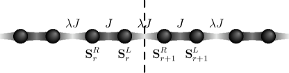
Figure 4: Schematic representation of the dimerized spin chain. Dark bonds stand for the coupling $J$ between two $S=\nicefrac{{1}}{{2}}$ spins forming a dimer, light bonds denote the variable inter-dimer coupling $\lambda J$. The dashed line indicates an axis of reflection symmetry.

In the previous section, we studied the truncation error for a zero-dimensional illustrative model. To illustrate the applicability of the truncation error for more relevant models, we extend our analysis to a one-dimensional system. Furthermore, this allows us to calculate and to compare the truncation errors of more complex real-space truncation schemes. As we will see, we have to use the triangle inequality again to arrive at error bounds in extended systems.

The model studied is the one-dimensional dimerized antiferromagnetic spin $S=\nicefrac{{1}}{{2}}$ Heisenberg chain with the Hamiltonian

$$H=J\sum\limits_{r}\left(\textbf{S}_{r}^{L}\cdot\textbf{S}_{r}^{R}+\lambda\textbf{S}_{r}^{R}\cdot\textbf{S}_{r+1}^{L}\right),\quad J>0.$$ (35)

In this notation, $\textbf{S}_{r}^{L}$ stands for the operator of the left spin in the dimer on position $r$ and $\textbf{S}_{r}^{R}$ for the right spin, see Fig. 4. The parameter $0\leq\lambda\leq 1$ denotes the relative strength of interdimer coupling. It is used as a control parameter similar to $\Gamma^{10}$ in Sect. III.

In the limit of $\lambda=0$, the system consists of isolated dimers. The ground state is given by a product state of singlets with a ground state energy of $\frac{E_{0}}{N}=-\frac{3}{4}J$ per dimer. The local $S=1$ excitations form equidistant spectrum with an increment of $J$.

For rising interdimer coupling, the excitations can be described by gapped spin $S=1$ quasiparticles called triplons Schmidt and Uhrig (2003). They can be seen as triplets with magnetic polarization cloud. In the limit $\lambda=1$, the gap closes and the correlations decay algebraically des Cloizeaux and Gaudin (1966); Yang and Yang (1966a, b); Faddeev and Takhtajan (1981); Klümper (1998); Sachdev (1999). For $\lambda=1$, the system is the well-known homogeneous spin chain exactly solved 1931 by Bethe Bethe (1931) by what was henceforth called Bethe ansatz. The ground state energy for the infinite chain was calculated by Hulthén Hulthén (1938) and takes the value $\nicefrac{{1}}{{2}}-2\ln 2$ per dimer and $J$.

With respect to the limit of isolated dimers, we choose for dimer $r$ a local basis of singlet/triplet states

$$\left|s\right\rangle_{r} =\frac{1}{\sqrt{2}}\left(\left|\uparrow\downarrow\right\rangle-\left|\downarrow\uparrow\right\rangle\right)\$$ (36a)

$$\left|x\right\rangle_{r} =\frac{-1}{\sqrt{2}}\left(\left|\uparrow\uparrow\right\rangle-\left|\downarrow\downarrow\right\rangle\right)\ = \ t^{\dagger}_{x,r} \left|s\right\rangle_{r}$$ (36b)

$$\left|y\right\rangle_{r} =\frac{i}{\sqrt{2}}\left(\left|\uparrow\uparrow\right\rangle+\left|\downarrow\downarrow\right\rangle\right)\ = \ t^{\dagger}_{y,r} \left|s\right\rangle_{r}$$ (36c)

$$\left|z\right\rangle_{r} =\frac{1}{\sqrt{2}}\left(\left|\uparrow\downarrow\right\rangle+\left|\downarrow\uparrow\right\rangle\right)\ = \ t^{\dagger}_{z,r} \left|s\right\rangle_{r}$$ (36d)

as in the bond operator representation Chubukov (1989a, b); Sachdev and Bhatt (1990). We define the reference state as the product state of singlets on each site

$$\left|0\right\rangle:=\bigotimes\limits_{r}\left|s\right\rangle_{r}.$$ (37)

The triplet operators are defined by

$$t^{\dagger}_{\alpha,r} :=\left|\alpha\right\rangle_{r}\left\langle s\right|_{r}$$ (38a)

$$t^{\phantom{\dagger}}_{\alpha,r} :=\left|s\right\rangle_{r}\left\langle\alpha\right|_{r}.$$ (38b)

Non-physical artifacts (e.g. states with two triplets on one dimer) are excluded. Therefore, the triplet operators obey the hard-core algebra

$$\left[t^{\phantom{\dagger}}_{\alpha,r},t^{\dagger}_{\beta,s}\right]=\delta_{rs}\delta_{\alpha\beta}\left(\mathbbm{1}-\sum\limits_{\gamma}t^{\dagger}_{\gamma,r}t^{\phantom{\dagger}}_{\gamma,r}\right)-\delta_{rs}t^{\dagger}_{\beta,r}t^{\phantom{\dagger}}_{\alpha,r}.$$ (39)

The normal-ordered products of triplet operators (monomials) together with the identity $\mathbbm{1}$ form the basis $\{A_{i}\}$ for all operators on the lattice. In this notation, the Hamiltonian reads

$$H=\sum\limits_{r} \ -\frac{3}{4}\mathbbm{1}+t^{\dagger}_{\alpha,r}t^{\phantom{\dagger}}_{\alpha,r}$$

$$\ +\frac{1}{4}\lambda\left(t^{\dagger}_{\alpha,r}+t^{\phantom{\dagger}}_{\alpha,r}\right)\left(t^{\dagger}_{\alpha,r+1}+t^{\phantom{\dagger}}_{\alpha,r+1}\right)$$

$$\ +\frac{i}{4}\lambda\epsilon_{\alpha\beta\gamma}\left(\left(t^{\dagger}_{\alpha,r}+t^{\phantom{\dagger}}_{\alpha,r}\right)t^{\dagger}_{\beta,r+1}t^{\phantom{\dagger}}_{\gamma,r+1}\right.$$ (40)

$$\ \left.-t^{\dagger}_{\beta,r}t^{\phantom{\dagger}}_{\gamma,r}\left(t^{\dagger}_{\alpha,r+1}+t^{\phantom{\dagger}}_{\alpha,r+1}\right)\right)$$

$$+\frac{1}{4}\lambda \left(t^{\dagger}_{\beta,r}t^{\phantom{\dagger}}_{\gamma,r}t^{\dagger}_{\gamma,r+1}t^{\phantom{\dagger}}_{\beta,r+1}-t^{\dagger}_{\beta,r}t^{\phantom{\dagger}}_{\gamma,r}t^{\dagger}_{\beta,r+1}t^{\phantom{\dagger}}_{\gamma,r+1}\right).$$

By the CUT the triplet states are mapped to re-normalized $S=1$ excitations (triplons).

The Hamiltonian (IV.1) has three different symmetries that can be used for simplification of the calculation as mentioned in Sect. I.4:

(i) The Hamiltonian (IV.1) is self-adjoint. Although this is not a symmetry in the strict sense of the word, it implies an additional constraint for the coefficients of $H$. Since quasiparticle creating and annihilating terms have to occur in pairs in any Hamiltonian, one of them can be chosen as representative for the pair. Thereby the number of coefficients to be tracked is reduced.

(ii) The Hamiltonian (IV.1) shares the reflection symmetry of the chain $r\to-r$, see Fig. 4. In addition, all left-spin and right-spin operators have to be swapped implying $t^{\phantom{\dagger}}_{\alpha,r}\leftrightarrow-t^{\phantom{\dagger}}_{\alpha,r}$ in the triplon notation .

(iii) The Hamiltonian (35) is invariant under SU(2) rotations in spin space. Due to this invariance, the Hamiltonian written in the triplet algebra (IV.1) can be decomposed into symmetric combinations of terms. The terms in a symmetric combination differ only by permutations of triplet polarizations up to a sign factor. The superoperator $\sum_{G}$ to build the symmetric combination of a maximally asymmetric representative reads

$$\sum_{xyz}=\sum_{xy}\sum_{\text{cyc}}=\left(\mathbbm{1}+\widehat{S}_{xy}\right)\left(\mathbbm{1}+\widehat{S}_{\text{cyc}}+\widehat{S}_{\text{cyc}}^{2}\right),$$ (41)

where the cyclic permutations of triplet polarizations is denoted by $\widehat{S}_{\text{cyc}}$ and the exchange of the polarizations $x$ and $y$ with a negative sign factor for each triplet operator reads $\widehat{S}_{xy}$.

IV.2 Real-space truncation

For an extended system, the omission of processes that create or annihilate more than $N$ triplons as mentioned in Sect. I.3 can be insufficient because the number of remaining terms is still infinite. For example, even by restricting to processes of at most two triplons, an infinite number of independent terms varying by range can emerge in the course of the flow. Since an energy gap implies a finite correlation length, it is an adequate choice to neglect all processes that exceed a given range $d_{\text{max}}$. In a one dimensional system, the range can easily be defined as the distance of the rightmost and leftmost triplet operator in a term.

In particular, it has turned out to be advantageous to use a combination of both the quasiparticle and the range criterion as truncation scheme Reischl (2006); Fischer et al. (2010). For the most important processes of low quasiparticle number, e.g., the hopping of triplons, a long range is allowed for to preserve most of the relevant physics. For more complex processes of more quasiparticles only a shorter range can be considered because their number increases much more steeply with range. But since more quasiparticles are required for such terms to become active the reduced range does not need to imply a reduced accuracy.

In view of the above considerations we classify terms by the sum $n$ of created and annihilated quasiparticles. For each value of $n$ a specific maximal range $d_{n}$ is defined. The complete truncation scheme can be written as $\textbf{d}=\left(d_{2},d_{3}\dots d_{2N}\right)$ where at most $N$ quasiparticles may be created or annihilated. No maximal range needs to be specified for $n=1$ because those terms always have range zero and their number is, due to translation symmetry, restricted to the six local creation and annihilation operators. Furthermore, without magnetic field no single annihilation or creation of triplons takes place due to the conservation of the total spin.

IV.3 Triangle inequality

To calculate the truncation error according to Eq. (20b), the norm of the inhomogeneity

$$\kappa(\ell)=\sum\limits_{A_{i}}\kappa_{A_{i}}(\ell)A_{i}$$ (42)

has to be calculated. Its coefficients $\kappa_{A_{i}}$ are obtained using Eq. (13) from the coefficients of $H^{\prime}$ by evaluating the terms of the commutator that are discarded in the truncation scheme. The precise calculation of $\left|\left|\kappa\right|\right|$ is not feasible for large systems because the effort to calculate the maximal eigen-value is too large. Since we are only interested in an upper bound, we apply the triangle inequality again to reach

$$\left|\left|\kappa(\ell)\right|\right|=\left|\left|\sum\limits_{A_{i}}\kappa_{A_{i}}(\ell){A_{i}}\right|\right|\leq\sum\limits_{{A_{i}}}\left|\kappa_{A_{i}}(\ell)\right|\left|\left|A_{i}\right|\right|.$$ (43)

In this way, we define an upper bound $\widetilde{\Lambda}_{H}$ or the truncation error

$$\widetilde{\Lambda}_{H}(\ell)=\sum\limits_{{A_{i}}}\int\limits_{0}^{\ell}\left|\kappa_{A_{i}}(\ell^{\prime})\right|\mathsf{d}\ell^{\prime}\left|\left|A_{i}\right|\right|\geq\Lambda_{H}(\ell).$$ (44)

Therefore, $\widetilde{\Lambda}_{H}$ is also an upper bound for $\Delta E_{0}$ and $\Delta E_{\text{max}}$, although it is less strict than $\Lambda_{H}$.

Recall that our basis operators $A_{i}$ are normal-orderd products of hard-core-boson creation and annihilation operators. It turns out that in this case the spectral norm $\left|\left|A_{i}\right|\right|$ can be calculated easily since the product ${A_{i}}^{\dagger}{A_{i}}$ is already diagonal with respect to the dimer eigen-states. It is a product of local triplon density terms. Thus ${A_{i}}^{\dagger}{A_{i}}$ has the eigen-value unity for all configurations having triplons with the polarization of the local triplon density operators on each site of the cluster of ${A_{i}}$ . For different occupations, ${A_{i}}^{\dagger}{A_{i}}$ has the eigen-value zero. Therefore the spectral norm for all elements of the operator basis $\{A_{i}\}$ is unity.

IV.4 Optimization using symmetries

As pointed out in Sect. I.4, exploiting symmetries reduces the computational effort for the S-CUT method significantly. In addition, symmetries can be used to reduce the bound $\widetilde{\Lambda}$. To see this, we write $\Lambda$ using the basis of representatives $\{C_{i}\}$ of operator monomials

$$\Lambda_{H}(\ell) =\sum\limits_{C_{i}}\int\limits_{0}^{\ell}\left|\left|\kappa_{C_{i}}(\ell^{\prime})\sum_{G}{C_{i}}\right|\right|\mathsf{d}\ell^{\prime}$$ (45a)

$$\leq\sum\limits_{C_{i}}\int\limits_{0}^{\ell}\left|\kappa_{C_{i}}(\ell^{\prime})\right|\mathsf{d}\ell^{\prime}\cdot\left|\left|\sum_{G}{C_{i}}\right|\right|=:\widetilde{\Lambda}_{H}(\ell).$$ (45b)

We use the triangle inequality again to decompose $\left|\left|\sum_{G}{C_{i}}\right|\right|$ into the weight $w_{C_{i}}$ which denote the number of terms generated by $\sum_{G}$ multiplied by the norm of the representative. This yields

$$\widetilde{\Lambda}_{H}(\ell)=\left(\int\limits_{0}^{\ell}\left|\kappa_{C_{i}}(\ell^{\prime})\right|\mathsf{d}\ell^{\prime}\right)w_{C_{i}}\left|\left|{C_{i}}\right|\right|.$$ (46)

If, however, we avoid the triangle inequality for the fully symmetric combination of basis operators we obtain a better, stricter upper bound. This enters Eq. (46) by replacing $w_{C_{i}}$ by a reduced effective weight $w^{G}_{C_{i}}$. In order to determine this reduction, we have to calculate the relation between the norm of the fully symmetric combination and the norm of a single representative analytically

$$\left|\left|\sum_{G}{C_{i}}\right|\right|=:w^{G}_{C_{i}}\left|\left|{C_{i}}\right|\right|.$$ (47)

The effective weight factor $w^{G}_{C_{i}}$ allows us to modify Eq. (46) to calculate the improved truncation bound $\widetilde{\Lambda}^{G}$. In presence of multiple symmetries, it is possible to improve the weight with respect to only some selected symmetries. The other symmetries can be treated by using the triangle inequality as done in Eq. (46). They continue to enter the combined weight by an additional factor.

As an example, we consider the self-adjointness to reach the improved truncation bound $\widetilde{\Lambda}^{\dagger}_{H}$. To determine its weight, it is useful to decompose the action of a representative

$$C=\left|c_{1}\right\rangle\left\langle c_{2}\right|\bigotimes\limits_{r\notin\text{cluster}}\mathbbm{1}$$ (48)

into the non-trivial action on its cluster and into the identity on the rest of the system. Since $C$ is a normal-ordered product of hard-core-boson operators, the action on its cluster is given by only one non-vanishing matrix element.

To build the corresponding symmetric combination $\sum_{G}C$, we have to distinguish two cases:

(i) $\left|c_{1}\right\rangle=\left|c_{2}\right\rangle$ If $C$ is self-adjoint, it is already a symmetric combination and thushas a weight factor of unity in both cases, i.e., using and not using the self-adjointness.

(ii) $\left|c_{1}\right\rangle\neq\left|c_{2}\right\rangle$ In this case, the symmetric combination for $C$ reads

$$\sum_{G}C=\left(\mathbbm{1}+\widehat{A}\right)C=\left(\left|c_{1}\right\rangle\left\langle c_{2}\right|+\left|c_{2}\right\rangle\left\langle c_{1}\right|\right)\bigotimes\limits_{r\notin\text{cluster}}\mathbbm{1}.$$ (49)

Due to our choice of basis, both $\left|c_{1}\right\rangle$ and $\left|c_{2}\right\rangle$ are eigen-states of local triplet density operators and therefore orthogonal, which implies the maximal eigen-value of 1 for $\left|c_{1}\right\rangle\left\langle c_{2}\right|+\left|c_{2}\right\rangle\left\langle c_{1}\right|$. Hence $\|\left|c_{1}\right\rangle\left\langle c_{2}\right|\|=1$ and $\|\left|c_{1}\right\rangle\left\langle c_{2}\right|+\left|c_{2}\right\rangle\left\langle c_{1}\right|\|=1$ which implies a gain of a factor of 2 if the triangle inequality is avoided which would have led to $\|\left|c_{1}\right\rangle\left\langle c_{2}\right|+\left|c_{2}\right\rangle\left\langle c_{1}\right|\|\leq\|\left|c_{1}\right\rangle\left\langle c_{2}\right|\|+\|\left|c_{2}\right\rangle\left\langle c_{1}\right|\|=2$. As an example, we consider the representative $t^{\dagger}_{x,1}t^{\phantom{\dagger}}_{x,1}t^{\dagger}_{y,2}$. On its cluster $\{1,2\}$ it stands for a transition from $\left|x_{1}s_{2}\right\rangle$ to $\left|x_{1}y_{2}\right\rangle$. The matrix representation for the action of its symmetric combination

$$\sum_{G}t^{\dagger}_{x,1}t^{\phantom{\dagger}}_{x,1}t^{\dagger}_{y,2}=\left(\left|x_{1}y_{2}\right\rangle\left\langle x_{1}s_{2}\right|+\left|x_{1}s_{2}\right\rangle\left\langle x_{1}y_{2}\right|\right)\bigotimes\limits_{r\notin\{1,2\}}\mathbbm{1}$$ (50)

has zero matrix elements except for a $2\times 2$ block with the eigen-values -1 and +1.

In conclusion, using self-adjointness to gain an effective weight $w^{\dagger}$ saves a factor of 2 for non-symmetric terms.

This effective weight can be improved further by considering spin symmetry. The complete symmetry group with respect to all permutations of triplet polarizations can be decomposed into the subgroup of cyclic permutations and the subgroup of the transposition of $x$ and $y$ triplets $\widehat{S}_{xy}$ plus the identity. For simplicity, we concentrate on the latter one only and calculate the truncation bound $\widetilde{\Lambda}_{H}^{\dagger,xy}$. The matrix associated with the $\sum_{G}C$ action on its cluster can have up to four non-vanishing matrix elements , i.e., four states of the cluster have to be taken into account. The representatives can be classified by the specific action of $\sum_{G}$ needed to obtain the corresponding fully symmetric combination:

$\sum_{G}=\mathbbm{1}$: These highly symmetric representatives (e.g. $t^{\dagger}_{z,1}t^{\phantom{\dagger}}_{z,1}$) are invariant under both $\widehat{A}$ and $\widehat{S}_{xy}$. They have weight $w^{\dagger,xy}$ unity.

$\sum_{G}=\mathbbm{1}+\widehat{A}$: These representatives are not self-adjoint, but invariant under either transposition of $x$ and $y$ (e.g. $t^{\phantom{\dagger}}_{z,1}$) or under the combination of transposing and adjunction (e.g. $t^{\dagger}_{x,1}t^{\phantom{\dagger}}_{y,1}$). As discussed previously, the weight $w^{\dagger,xy}$ takes the value of 1 instead of 2.

$\sum_{G}=\mathbbm{1}+\widehat{S}_{xy}$: For representatives that are self-adjoint, but not invariant under transposition (e.g. $t^{\dagger}_{x,1}t^{\phantom{\dagger}}_{x,1}$), the weight $w^{\dagger,xy}$ is reduced to the value 1 instead of 2 as well.

$\sum_{G}=\left(\mathbbm{1}+\widehat{A}\right)\left(\mathbbm{1}+\widehat{S}_{xy}\right)$: In this asymmetric case, the norm of the symmetric combination can be either one (e.g. $t^{\dagger}_{x,1}t^{\phantom{\dagger}}_{y,2}$) or $\sqrt{2}$ (e.g. $t^{\dagger}_{x,1}$). Therefore, $w^{\dagger,xy}=\sqrt{2}$ can be used instead of $w=4$ .

The weights can be improved by exploiting further symmetries, e.g., cyclic spin permutations or reflection symmetry. But the complexity of the necessary case-by-case analysis rises considerably. Especially the use of point group symmetries of the lattice is complicated because the cluster of monomials linked by a point group do not need to be identical. Thus the inclusion of point group symmetries in the calculation of the bounds is beyond the scope of this article.

IV.5 Results for an infinite system

Figure 5: Renormalized truncation bound per dimer $\widetilde{\Lambda}_{H}$ and reduced bounds $\widetilde{\Lambda}_{H}^{\dagger}$ (exploiting self-adjointness) and $\widetilde{\Lambda}_{H}^{\dagger,xy}$ (exploiting self-adjointness and $xy$ symmetry) vs. the interdimer coupling $\lambda$ for the ground state generator using the truncation scheme $\textbf{d}=\left(8,6,6,3,3\right)$.

Figure 6: Renormalized reduced truncation bounds per dimer $\widetilde{\Lambda}_{H}^{\dagger,xy}$ vs. interdimer coupling $\lambda$ for ground state and particle conserving generator using various truncation schemes.

$\widehat{\eta}$	d	$\left|\Delta E_{0}\right|$	$\widetilde{\Lambda}_{H}$	$\widetilde{\Lambda}_{H}^{\dagger}$	$\widetilde{\Lambda}_{H}^{\dagger,xy}$
$\widehat{\eta}_{\text{pc}}$	$(6,3,3)$	0.01739	439.37	219.93	156.74
$\widehat{\eta}_{\text{pc}}$	$(8,6,6,3,3)$	0.00032	49926.1	24974.8	17660.2
$\widehat{\eta}_{\text{gs}}$	$(6,3,3)$	0.02675	23.51	11.75	8.41
$\widehat{\eta}_{\text{gs}}$	$(8,6,6,3,3)$	0.00915	149.31	74.68	52.98
$\widehat{\eta}_{\text{gs}}$	$(9,7,7,4,4)$	0.00948	169.32	84.67	60.04

Table 1: Numerical values for the renormalized truncation bound per dimer $\widetilde{\Lambda}_{H}$ and reduced bounds $\widetilde{\Lambda}_{H}^{\dagger}$, $\widetilde{\Lambda}_{H}^{\dagger,xy}$ for $\lambda=1$ for the generators and the truncation schemes used in Fig. 6. The inaccuracies of the ground state energy $\left|\Delta E_{0}\right|$ are calculated with respect to the analytical result Hulthén (1938).

Figure 5 shows the bound $\widetilde{\Lambda}_{H}$ defined in Eq. (46) for the infinite dimerized Heisenberg chain using the ground state generator scheme $\widehat{\eta}_{\text{gs}}$ Fischer et al. (2010) defined in (7) and the truncation scheme $\textbf{d}=(8,6,6,3,3)$ as function of the interdimer coupling $\lambda$. For rising values of $\lambda$, the truncation bound increases drastically similar to the behavior observed for the illustrative model. But it attains a significantly higher absolute value finally.

For weak interdimer coupling $\lambda\lesssim 0.1$, the error bound for the ground state energy given by $\widetilde{\Lambda}$ is useful as a rigorous bound. But this estimate becomes inappropriate for medium and strong coupling since the $\widetilde{\Lambda}$ grows rapidly to the same magnitude as $E_{0}$ and beyond so that it does no longer represent a meaningful bound.

For $\lambda=1$ the analytical result can be used as reference to determine the error of the ground state energy per dimer $\left|\Delta E_{0}\right|$ determined as the renormalized vacuum energy of the CUT, see Tab. 1. This relative error is only $1.04\%$. In contrast, the truncation bound $\widetilde{\Lambda}_{H}$ exceeds the ground state energy by several orders of magnitude.

This discrepancy stems from the fact that the truncation error $\Lambda_{H}$ measures truncation effects of the entire transformation, not only of the inaccuracies of ground state energy in particular. The extensive use of the triangle inequality to calculate the truncation bound $\widetilde{\Lambda}$ enhances this difference additionally, although it can be reduced exploiting symmetry. The interesting question which effect dominates is postponed to the study of a finite system below where all quantities are numerically accessible.

The use of the adjunction symmetry reduces the bound by a factor of about two, and the use of $xy$ symmetry reduces it by an additional factor of about $\sqrt{2}$. In both cases, exploiting the symmetry pays in decreasing the bound close to the optimum which can be achieved for terms with the lowest symmetry. Since terms with low symmetry occur much more frequently than symmetric ones, the error bound is reduced efficiently by exploiting symmetries. However, the gain achieved in this way can not overcome the tremendous factor (orders of magnitude) between the upper bound and to the error of the ground state energy.

In the extended system, various truncation schemes of different quality and computational effort can be used. Figure 6 shows the truncation bound $\widetilde{\Lambda}_{H}^{\dagger,xy}$ for different truncations and generator schemes. Besides the particle conserving generator $\widehat{\eta}_{\text{pc}}$ the ground state decoupling generator $\widehat{\eta}_{\text{gs}}$ is applied, for details see Ref. Fischer et al., 2010. The numerical values for $\lambda=1$ including the difference to the exact ground state energy are given in Tab. 1.

In general, the particle conserving generator scheme $\widehat{\eta}_{\text{pc}}$ yields significantly higher truncation bounds than $\widehat{\eta}_{\text{gs}}$, although the inaccuracies of the calculated ground state energies are lower (using equal truncation schemes d). This is due to the fact that $\widehat{\eta}_{\text{pc}}$ performs a more comprehensive reordering of the quasiparticle subspaces and includes much more terms than $\widehat{\eta}_{\text{gs}}$. This implies a higher impact of truncation errors. Much more terms emerge in the evaluation of the commutator and have to be incorporated in $\kappa$ resulting in a larger differential equation system with much more coefficients.

The dependence on the truncation scheme is more complex. For weak coupling, looser truncation schemes imply lower truncation error bounds than stricter schemes. This is what one expects naively since the inclusion of more and more terms, hence a less strict truncation, should describe the system better and better. Thus the truncation error should decrease.

But this relation can be inverted for strong coupling although the looser schemes reproduce the analytical result for the ground state energy with much higher accuracy for both generator schemes as seen for $(6,3,3)$ and $(8,6,6,3,3)$. We call this phenomenon the truncation paradoxon because it seems to be paradoxical at first glance. We stress that it does not represent a logical contradiction but only a counterintuitive behaviour.

On second thought, one realizes that the use of a looser truncation scheme increases the number of terms in $\kappa$ drastically. For instance, an increase from 30.972 for $(6,3,3)$ to 16.777.215 representatives for $(8,6,6,3,3)$ is found in the $\widehat{\eta}_{\text{pc}}$ scheme. Irrespective of the consequences to the spectral norm of $\kappa$, this massive increase of terms has a big impact on the bound $\widetilde{\Lambda}$ which relies on the triangle inequality to bound each of these terms separately. Hence the bound is so large simply because it is very loose.

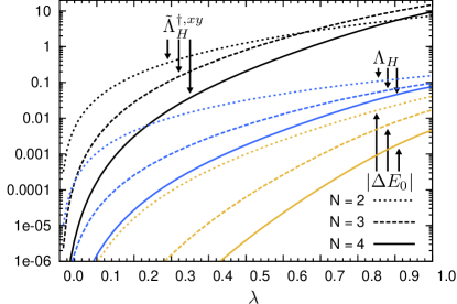
Figure 7: (Color online) Renormalized truncation bound per dimer $\widetilde{\Lambda}_{H}^{\dagger,xy}$, exact renormalized truncation error per dimer $\Lambda_{H}$ and error of ground state energy per dimer $\left|\Delta E_{0}\right|$ vs. interdimer coupling $\lambda$ for the ground state generator considering at most $N$ triplon operators per term.

$N$	$\left|\Delta E_{0}\right|$	$\Lambda_{H}$	$\widetilde{\Lambda}_{H}$	$\widetilde{\Lambda}_{H}^{\dagger}$	$\widetilde{\Lambda}_{H}^{\dagger,xy}$
2	0.04109	0.1556	20.34	10.17	7.28
3	0.01709	0.0964	41.87	20.93	14.86
4	0.00465	0.0768	26.78	13.39	9.48

Table 2: Error of ground state energy per dimer $\left|\Delta E_{0}\right|$, exact renormalized truncation error per dimer $\Lambda_{H}$ and renormalized truncation bounds per dimer $\widetilde{\Lambda}_{H}$, $\widetilde{\Lambda}_{H}^{\dagger}$ and $\widetilde{\Lambda}_{H}^{\dagger,xy}$ for $\lambda=1$ using the ground state generator scheme $\widehat{\eta}_{\text{gs}}$ considering at most $N$ triplon operators per term.

IV.6 Results for a finite extended system

The question arises whether the truncation paradox is caused by the extensive use of triangle inequality to determine the bound $\widetilde{\Lambda}$, or whether it is an intrinsic characteristics of the truncation error $\Lambda$ itself. To investigate this issue, it is necessary to determine the exact truncation error $\Lambda$ without use of the triangle inequality. Thus an exact diagonalization of $\kappa$ is required. This restricts us to the investigation of a finite chain segment.

In the following, we study the periodic, dimerized Heisenberg chain consisting of five dimers. In view of the small size of the system, we use the maximal number $N$ of interacting triplons as only truncation criterion. No extensions are considered.

Figure 7 shows the truncation bound $\widetilde{\Lambda}_{H}^{\dagger,xy}$, the exact truncation error $\Lambda$ and the deviation of the ground state energy $\left|\Delta E_{0}\right|$ vs. $\lambda$. The values for $\lambda=1$ are given in Tab. 2. It turns out that both the calculation of the exact truncation error $\Lambda_{H}$ and the extensive use of the triangle inequality contribute to the very large values of $\widetilde{\Lambda}_{H}^{\dagger,xy}$. For small values of $\lambda$, the large value of $\Lambda_{H}$ dominates the truncation bound $\widetilde{\Lambda}_{H}^{\dagger,xy}$ while for large values of $\lambda$, the approximation using the triangle inequality to bound the very many arising terms contributes most.

In a direct comparision, the exact truncation error $\Lambda_{H}$ is overestimated by the bound $\widetilde{\Lambda}_{H}^{\dagger,xy}$ using the triangle inequality by two orders of magnitudes, even though symmetries are used. Nevertheless, $\Lambda_{H}$ is still considerably higher than the deviation of ground state energy. In particular, it exceeds $\left|\Delta E_{0}\right|$ by several orders of magnitudes for small $\lambda$. Here we have to keep in mind that the truncation error does not only measure the inaccuracies of ground state energy, but the effect of truncation to the entire transformation of the Hamiltonian.

In contrast to the double hard-core boson model, no deviations in the maximal energy eigen-value were observed (not shown). This is explained by the fact that the fully polarized state is still an exact eigen-state of the Hamiltonian (35).

For high values of $\lambda$, the truncation paradox occurs again because the truncation error bound $\widetilde{\Lambda}_{H}^{\dagger,xy}$ for the three-triplon and the four-triplon truncation exceeds the truncation error bound of the two-triplon truncation. The exact truncation error $\Lambda_{H}$ does not display any paradoxical behaviour. Hence we conclude that the extensive use of the triangle inequality is at the basis of the truncation paradox.

V Summary

In this work, we presented a mathematically rigorous framework to bound effects of truncation in self-similar continuous unitary transformations a priori. The difference ${H^{\prime\prime}}=H-H^{\prime}$ between a unitarily transformed Hamiltonian $H$ and the Hamiltonian $H^{\prime}$ obtained from the truncated calculation is captured by an inhomogeneous flow equation depending only on the truncated terms. We defined the scalar truncation error $\Lambda$ by the norm of the truncated terms $\left|\left|\kappa\right|\right|$. It provides an upper bound for the norm of the difference $\left|\left|H^{\prime\prime}\right|\right|$. A completely analogous bound is derived for observables as well.

Using the spectral norm, the truncation error implies an upper bound for the deviation of the minimal and maximal eigen-value of the observable under study, which is caused by truncation. In particular, we derived a rigorous a priori bound for the error of ground state energy.

The analysis of the double hard-core boson model showed that the norm of the difference ${H^{\prime\prime}}$ is bounded and approximated very well by the truncation error. Despite the large difference to $\left|\Delta E_{0}\right|$, the truncation error $\Lambda_{H}$ provided a good measure for the deviation in the highest excited level $\left|\Delta E_{\text{max}}\right|$. This could be understood by the special feature of the truncation scheme that primarily affected the highest excited level.

For practical use in extended systems, an upper bound $\widetilde{\Lambda}$ for the truncation error is calculated using the triangle inequality. The direct calculation of $\left|\left|\kappa\right|\right|$ is not feasible – even impossible for infinite systems – because it would require an exact diagonalization in the Hilbert space of the entire system.

In both systems studied, the double hard-core boson model and the extended dimerized spin chain , the bound provided by truncation error $\Lambda_{H}$ turned out to overestimate the actual inaccuracies of the ground state energy significantly. This is an inevitable consequence of the fact that the truncation error is a measure for the non-unitarity of the whole transformation. Therefore it is sensitive to distortions of all eigen-values and eigen-states.

A comparison of various bounds for finite dimerized spin chain segments showed that the truncation bound $\widetilde{\Lambda}_{H}$ overestimates the real truncation error $\Lambda_{H}$ by orders of magnitudes. Furthermore, a truncation paradoxon was observed: Looser, i.e., better, truncation schemes implied higher truncation bounds. In the finite system studied using the ground state generator, this paradoxon did not occur for the exact truncation errors.

The truncation bound can be improved efficiently exploiting symmetries of the Hamiltonian and its hermitecity. By using the transposition of the triplon polarizations $x$ and $y$ and the hermitecity, we were able to reduce the bound by a factor $\approx 2\sqrt{2}$. To overcome the high difference to the truncation error $\Lambda$, much more sophisticated approximations would be needed. Additional symmetries available are the cyclic spin permutation, the reflection symmetry, and the translation symmetry. We do not see a way to exploit the powerful translation symmetry completely for the improvement of the bounds because this requires finding bounds for operators in very large or infinite systems. But larger subsets of terms of restricted range could indeed be analyzed on larger clusters. The calculation of $H^{\prime\prime}$ in an extended system is left for further investigation.

The analysis presented here provides a better understanding of truncation errors in continuous unitary transformations. We are confident that it serves as seed for stricter a priori error bounds in the future.

Appendix A Effective system size

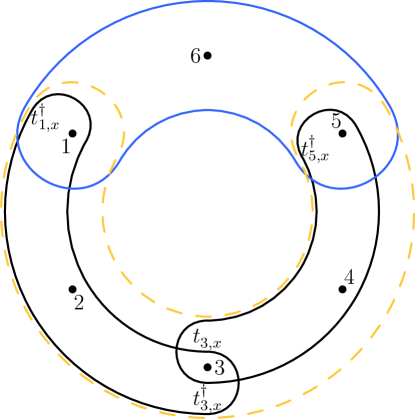
Figure 8: (Color online) Schematic representation of the generation of a term which complies with the truncation scheme with $d_{\text{max}}=2$ only due to the finiteness of the systeme with size $l=6$. Following the hard-core-algebra, the commutator of the terms $t^{\dagger}_{1,x}t^{\dagger}_{3,x}$ and $t_{3,x}t^{\dagger}_{5,x}$ (black) generates several terms, see Eq. (51), with range 4 that are truncated (orange/gray and dashed), but the term $t_{1,x}t^{\dagger}_{5,x}$ is not truncated due to a ‚wrap-around‘ effect (blue/gray).

$L$	$\lambda=0.5$	$\lambda=1.0$
3	-0.7821366540	-0.9342579563
4	-0.7778813863	-0.9019258071
5	-0.7770436419	-0.8836215559
6	-0.7768700368	-0.8745235739
7	-0.7768649893	-0.8740959679
8	-0.7768649893	-0.8740959679
9	-0.7768649893	-0.8740959679
10	-0.7768649893	-0.8740959679

Table 3: Ground state energies per dimer $E_{0}$ for the finite dimerized Heisenberg chain obtained by S-CUT using a real-space truncation scheme for systems of different numbers of dimers $n$ and different interdimer couplings $\lambda$. The maximum untruncated range is set to $d_{\text{max}}=2$, the corresponding effective system size $L_{\text{fin}}$ is 7. Beyond this size, the calculated quantities become independent of the system size.

In Sect. II.1 we mentioned that using a real-space truncation scheme implies an effective system size $L_{\text{fin}}$ that disguises the differences between infinite and finite periodic systems with a size of at least $L_{\text{fin}}$. The coefficients of representatives calculated by a truncated S-CUT become independent of the physical system size. At first glance, this seems to be puzzling. But one has to look in detail where the finite system size enters in the calculation of the flow equation.

For clarity, we focus on a one-dimensional system, although the argument can be generalized to higher dimensions. Let $d_{\text{max}}$ be the maximal range of the untruncated terms and $l$ the systems size. In order to keep the translational invariance of the infinite system also for a finite chain, periodic boundary conditions must be chosen. By evaluation of the flow equation (2), the range of the terms stemming from the commutator $\left[\eta(\ell),H(\ell)\right]$ becomes important.

For an infinite system, the issue is clear because the maximum range of the commutator of two processes of range $d_{1}$ and $d_{2}$ is given by the sum $d_{\text{comm}}=d_{1}+d_{2}$ $d_{c}=d_{1}+d_{2}$. In a periodic system the range of a term is a more complex issue. The cluster of a term ambiguous because each site may be chosen to be the leftmost site.. As an example, the range of the term $t^{\dagger}_{1,x}t^{\dagger}_{5,x}$ in a system of six dimers can be defined to be either 4 or 2, see Fig. 8. To remove this ambiguity the most plausible prescription is to define the range of a term to be the minimum range of all possible choice of the leftmost site.

If the maximal range in the generator and in the Hamiltonian is $d_{\text{max}}$ the maximal range of terms stemming from the commutator is given by $d_{\text{comm,max}}=2d_{\text{max}}$. Due to the locality of the algebra, the clusters of both terms have to share at least one common site as can be seen in Fig. 8. So for smaller systems $L\leq d_{\text{comm,max}}$ the result of the commutation is strongly influenced by the finite size. If the system is larger than $d_{\text{comm,max}}$, the terms from the commutator are identical to those in the infinite system. But even then a wrap-around can influence the range which is actually attributed to a term resulting from the commutator. As an example we consider the commutator

$$\begin{split}&\left[t^{\dagger}_{1,x}t^{\dagger}_{3,x},t^{\phantom{\dagger}}_{3,x}t^{\dagger}_{5,x}\right]=-t^{\dagger}_{1,x}t^{\dagger}_{5,x}+2t^{\dagger}_{1,x}t^{\dagger}_{3,x}t^{\phantom{\dagger}}_{3,x}t^{\dagger}_{5,x}\\ &\qquad+t^{\dagger}_{1,y}t^{\dagger}_{3,y}t^{\phantom{\dagger}}_{3,y}t^{\dagger}_{5,y}+t^{\dagger}_{1,z}t^{\dagger}_{3,z}t^{\phantom{\dagger}}_{3,z}t^{\dagger}_{5,z}.\end{split}$$ (51)

In the infinite system, each of the terms on the right-hand side of (51) would be truncated since their range 4 exceeds the maximal range set to 2. But in the periodic system, the range of the contribution $-t^{\dagger}_{1,x}t^{\dagger}_{5,x}$ can be lower due to a ‚wrap-around‘ if the system is small enough, see Fig. 8.

In general, this anomalous range assignment due to a wrap-around can happen if the relation

$$L\leq d_{\text{comm,max}}+d_{\text{max}}=3d_{\text{max}}$$ (52)

is fullfilled. As a result one obtains the same differential equations for the representatives for all systems with a size of at least

$$L_{\text{fin}}=3d_{\text{max}}+1.$$ (53)

This included the infinite system. Hence $L_{\text{fin}}$ defines the effective size of a system treated with the maximal truncation range $d_{\text{max}}$.

For a numerical illustration, we examine the dependency of the ground state energy per dimer for the dimerized Heisenberg chain introduced in Sect. IV. We use the real-space truncation scheme with a maximal truncation length $d_{\text{max}}=2$ and no restrictions of the number of interacting triplons. This implies an effective system size $L_{\text{fin}}$ of 7 dimers according to (53). The results are given in Tab. 3. Clearly, the results are numerically identical for larger systems as predicted.

References

- Wegner (1994) F. Wegner, Ann. Physik 506, 77 (1994).
- Głazek and Wilson (1993) S. D. Głazek and K. G. Wilson, Phys. Rev. D 48, 5863 (1993).
- Głazek and Wilson (1994) S. D. Głazek and K. G. Wilson, Phys. Rev. D 49, 4214 (1994).
- Kehrein and Mielke (1997) S. K. Kehrein and A. Mielke, Ann. Physik 509, 90 (1997).
- Kehrein and Mielke (1998) S. Kehrein and A. Mielke, J. Stat. Phys. 90, 889 (1998).
- Uhrig and Normand (1998) G. S. Uhrig and B. Normand, Phys. Rev. B 58, R14705 (1998).
- Knetter and Uhrig (2000) C. Knetter and G. Uhrig, Eur. Phys. J. B 13, 209 (2000).
- Knetter (2003) C. Knetter, Ph.D. thesis, Universität zu Köln (2003).
- Reischl et al. (2004) A. Reischl, E. Müller-Hartmann, and G. S. Uhrig, Phys. Rev. B 70, 245124 (2004).
- Reischl (2006) A. A. Reischl, Ph.D. thesis, Universität zu Köln (2006).
- Lorscheid (2007) N. Lorscheid, Diploma thesis, Universität des Saarlandes (2007).
- Hamerla (2009) S. Hamerla, Diploma thesis, Technische Universität Dortmund (2009).
- Hamerla et al. (2010) S. A. Hamerla, S. Duffe, and G. S. Uhrig, 1008.0522 (2010).
- Lenz and Wegner (1996) P. Lenz and F. Wegner, Nucl. Phys. B 482, 693 (1996).
- Mielke (1997) A. Mielke, Ann. Physik 6, 215 (1997).
- Schmidt and Uhrig (2003) K. P. Schmidt and G. S. Uhrig, Phys. Rev. Lett. 90, 227204 (2003).
- Schmidt (2004) K. P. Schmidt, Ph.D. thesis, Universität zu Köln (2004).
- Schmidt and Uhrig (2005) K. Schmidt and G. Uhrig, Mod. Phys. Lett. B 19, 1179 (2005).
- Fischer et al. (2010) T. Fischer, S. Duffe, and G. S. Uhrig, NJP 12, 033048 (2010).
- Schmidt et al. (2008) K. P. Schmidt, S. Dusuel, and J. Vidal, Phys. Rev. Lett. 100, 057208 (2008).
- Dusuel et al. (2008) S. Dusuel, K. P. Schmidt, and J. Vidal, Phys. Rev. Lett. 100, 177204 (2008).
- Vidal et al. (2008) J. Vidal, K. P. Schmidt, and S. Dusuel, Phys. Rev. B 78, 245121 (2008).
- Wegner (2006) F. Wegner, J. Phys. A: Math. Gen. 39, 8221 (2006).
- Kehrein (2006) S. Kehrein, Springer Tr. Mod. Phys. 217, 1 (2006).
- Kehrein and Mielke (1994) S. K. Kehrein and A. Mielke, J. Phys. A: Math. Gen. 27, 4259 (1994).
- Mielke (1998) A. Mielke, Eur. Phys. J. B 5, 605 (1998).
- Dusuel and Uhrig (2004) S. Dusuel and G. Uhrig, J. Phys. A: Math. Gen. 37, 9275 (2004).
- Heidbrink and Uhrig (2002) C. Heidbrink and G. Uhrig, Eur. Phys. J. B 30, 443 (2002).
- Stein (1997) J. Stein, J. Stat. Phys. 88, 487 (1997).
- Stein (1998) J. Stein, Eur. Phys. J. B 5, 193 (1998).
- des Cloizeaux and Gaudin (1966) J. des Cloizeaux and M. Gaudin, J. Math. Phys. 7, 1384 (1966).
- Yang and Yang (1966a) C. N. Yang and C. P. Yang, Phys. Rev. 150, 321 and 327 (1966a).
- Yang and Yang (1966b) C. N. Yang and C. P. Yang, Phys. Rev. 151, 258 (1966b).
- Faddeev and Takhtajan (1981) L. D. Faddeev and L. A. Takhtajan, Phys. Lett. 85A, 375 (1981).
- Klümper (1998) A. Klümper, The European Physical Journal B 5, 677 (1998).
- Sachdev (1999) S. Sachdev, Quantum Phase Transitions (Cambridge University Press, 1999).
- Bethe (1931) H. Bethe, Z. Phys. A 71, 205 (1931).
- Hulthén (1938) L. Hulthén, Ark. Mat. Astron. Fys. 26A, 1 (1938).
- Chubukov (1989a) A. V. Chubukov, Pis’ma Zh. Éksp. Teor. Fiz. 49, 108 (1989a).
- Chubukov (1989b) A. V. Chubukov, JETP Lett. 49, 129 (1989b).
- Sachdev and Bhatt (1990) S. Sachdev and R. N. Bhatt, Phys. Rev. B 41, 9323 (1990).