Abstract

The analytical nonautonomous rogons are reported for the inhomogeneous nonlinear Schrödinger equation with variable coefficients in terms of rational-like functions by using the similarity transformation and direct ansatz. These obtained solutions can be used to describe the possible formation mechanisms for optical, oceanic, and matter rogue wave phenomenon in optical fibres, the deep ocean, and Bose-Einstein condensates, respectively. Moreover, the snake propagation traces and the fascinating interactions of two nonautonomous rogons are generated for the chosen different parameters. The obtained nonautonomous rogons may excite the possibility of relative experiments and potential applications for the rogue wave phenomenon in the field of nonlinear science.

Key words:  Inhomogeneous NLS equation with variable coefficients; Similarity transformation;

Rational-like solutions; Rogue waves; Rogons

PACS:  05.45.Yv; 42.65.-k; 42.81.Dp; 42.65.Sf; 03.75.Lm

The nonlinear Schrödinger (NLS) equation is a foundational model describing numerous nonlinear physical phenomenon in the field of nonlinear science such as optical solitons in optical fibres [2, 3, 4], solitons in the mean-field theory of Bose-Einstein condensates [5, 6, 7], and the rogue waves (RWs) (also known as freak waves, monster waves, killer waves, giant waves or extreme waves) in the nonlinear oceanography [8, 9, 10, 11]. RWs are single waves generated in the ocean with amplitudes much higher than the average wave crests around them [12, 13]. Recently, the RWs have attracted more and more attention from the point views of both theoretical analysis [22, 23, 24, 25, 26, 29, 30, 35] and experimental realization [14, 15, 31, 32, 33, 34]. The oceanic RWs can be, under the nonlinear theories of ocean waves, modelled by the dimensionless NLS equation [8, 9]

$$i\frac{\partial\psi}{\partial t}+\frac{1}{2}\frac{\partial^{2}\psi}{\partial x^{2}}+|\psi|^{2}\psi=0,\qquad\qquad\qquad\qquad\qquad\qquad\qquad\qquad\qquad\qquad$$ (1)

which describes the two-dimensional quasi-periodic deep-water trains in the lowest order in wave steepness and spectral width. In addition, it has been shown that the RWs can be generated in nonlinear optical systems and the term “optical rogue waves” was coined by observing optical pulse propagation in the generalized NLS equaiton [14, 15]. Some types of exact solutions of Eq. (1) have been presented to describe the possible formation mechanisms for the RW phenomenon such as the algebraic breathers (Peregrine solitons) [16], the time periodic breather (Ma solitons) [17], the space periodic breathers (Akhmediev breathers) [18, 19]. More recently, the Akhmediev breathers were also further studied [20, 21, 22, 23]. A possible mechanism for the formation of RWs was also exhibited by using two-dimensional coupled NLS equations  [25, 26, 27] describing the nonlinearly interacting two-dimensional waves in deep water. The three-dimensional mechanism of RW formation was studied in a late stage of the modulational instability of a perturbed Stokes deep-water wave [28]. Furthermore, the optical RWs were also found in the NLS equation with perturbing terms (the higher-order NLS equation with the third-order dispersion, self-steeping, and self-frequency shift)  [24]. Recently, the existence of matter RWs in Bose-Einstein condensates was predicted to either load into a parabolic trap or embed in an optical lattice [35].

Here we point out that based on physical similarities between the rogue waves and solitary waves, first observed by Russell in 1834 and further known as solitons by Zabusky and Kruskal in 1965 [46], we coin the word “Rogon” for each such “Rogue Wave” (or the word “Freakon” for the “Freak Wave”) if they reappear virtually unaffected in size or shape shortly after their interactions. Similarly, there also exist the corresponding new terms “oceanic rogons”, “optical rogons”, and “matter rogons” for the oceanic rogue waves [8, 9, 10, 11], optical rogue waves [14, 15, 22, 23, 24, 29, 30], and matter rogue waves [35], respectively.

To the best of our knowledge, there was no report on exact solutions related to the modified RWs (rogons) with variable functions before. In this Letter, we will extend the NLS equation (1) to the inhomogeneous NLS equation with variable coefficients, including group-velocity dispersion $\beta(t)$, linear potential $v(x,t)$, nonlinearity $g(t)$ and the gain/loss term $\gamma(t)$, in the form [36, 37, 38, 39]

$$i\frac{\partial\psi}{\partial t}+\frac{\beta(t)}{2}\frac{\partial^{2}\psi}{\partial x^{2}}+v(x,t)\psi+g(t)|\psi|^{2}\psi=i\gamma(t)\psi,\qquad\qquad\qquad\qquad\qquad\qquad$$ (2)

which is associated with $\delta\mathcal{L}/\delta\psi^{*}=0$, in which the Lagrangian density is written as $\mathcal{L}=i(\psi_{t}\psi^{*}-\psi\psi^{*}_{t})-\beta(t)|\psi_{x}|^{2}+g(t)|\psi|^{4}+2[v(x,t)-i\gamma(t)]|\psi|^{2}$, where $\psi\equiv\psi(x,t)$, and $\psi^{*}$ denotes the complex conjugate of the physical field $\psi$. Eq. (2) can be also known as the generalized Gross-Pitaevskii equation with variable coefficients for $\beta(t)=1$ [5, 6, 7, 45]. Our goal is focused on the first-order and second-order rational-like solutions of Eq. (2) to describe the possible formation mechanisms of optical RWs by using the similarity transformations [40, 41, 42, 43, 44, 45] and direct ansatz [22, 23]. Moreover, we analyze the dynamical behaviors of these solutions and interactions of two optical RWs (rogons) by choosing the different functions.

Similarity transformation and nonautonomous rogons— To investigate the analytical rational-like solutions of Eq.(2) related to the optical nonautonomous rogons, we employ the envelope field $\psi(x,t)$ in the gauge form [42, 43, 44, 45]

$$\begin{array}[]{l}\psi(x,t)=\left[\Psi_{{\rm R}}(x,t)+i\Psi_{\rm I}(x,t)\right]e^{i\varphi(x,t)}\end{array}$$ (4)

whose intensity can be written as $|\psi(x,t)|^{2}=|\Psi_{\rm R}(x,t)|^{2}+|\Psi_{\rm I}(x,t)|^{2}$, where $\Psi_{\rm R}(x,t),\ \Psi_{\rm I}(x,t)$ and $\varphi(x,t)$ are real functions of space-time $x,t$. The substitution of transformation (4) into Eq. (2) yields the system of coupled real partial differential equations with variable coefficients

$$\Psi_{{\rm R},t}+\frac{\beta(t)}{2}\left(\Psi_{{\rm I},xx}+2\varphi_{x}\Psi_{{\rm R},x}-\varphi_{x}^{2}\Psi_{\rm I}+\varphi_{xx}\Psi_{\rm R}\right)+[v(x,t)-\varphi_{t}]\Psi_{\rm I}+g(t)(\Psi_{\rm R}^{2}+\Psi_{\rm I}^{2})\Psi_{\rm I}-\gamma(t)\Psi_{\rm R}=0,\qquad\vspace{0.1in}$$ (5a)

$$-\Psi_{{\rm I},t}+\frac{\beta(t)}{2}\left(\Psi_{{\rm R},xx}-2\varphi_{x}\Psi_{{\rm I},x}-\varphi_{x}^{2}\Psi_{\rm R}-\varphi_{xx}\Psi_{\rm I}\right)+[v(x,t)-\varphi_{t}]\Psi_{\rm R}+g(t)(\Psi_{\rm R}^{2}+\Psi_{\rm I}^{2})\Psi_{\rm R}+\gamma(t)\Psi_{\rm I}=0.\qquad$$ (5b)

By introducing the new variables $\eta(x,t)$ and $\tau(t)$, we further utilize the following similarity transformations for the real functions $\Psi_{\rm R}(x,t)$, $\Psi_{\rm I}(x,t)$ and the phase $\varphi(x,t)$

$$\begin{array}[]{l}\Psi_{\rm R}(x,t)=A(t)+B(t)P(\eta(x,t),\tau(t)),\vspace{0.1in}\cr\Psi_{\rm I}(x,t)=C(t)Q(\eta(x,t),\tau(t)),\vspace{0.1in}\cr\varphi(x,t)=\chi(x,t)+\mu\tau(t),\end{array}$$ (9)

to system (5) such that we deduce the following similarity reduction

$$\eta_{xx}=0,$$ (10a)

$$\eta_{t}+\beta(t)\chi_{x}\eta_{x}=0,$$ (10b)

$$2\chi_{t}+\beta(t)\chi_{x}^{2}-2v(x,t)=0,$$ (10c)

$$2\sigma_{t}+[\beta(t)\chi_{xx}-2\gamma(t)]\sigma=0\ \ \ (\sigma=A,B,C),$$ (10d)

$$\tau_{t}BP_{\tau}+\frac{\beta(t)}{2}\eta_{x}^{2}CQ_{\eta\eta}-\mu\tau_{t}CQ+g(t)CQ[C^{2}Q^{2}+(A+BP)^{2}]=0,$$ (10e)

$$-\tau_{t}CQ_{\tau}+\frac{\beta(t)}{2}\eta_{x}^{2}BP_{\eta\eta}-\mu\tau_{t}(A+BP)+g(t)(A+BP)[C^{2}Q^{2}+(A+BP)^{2}]=0,\qquad\qquad$$ (10f)

where $\mu$ is a constant, and $\eta(x,t),\ \chi(x,t),\ A(t),\ B(t),\ C(t),\ \tau(t),\ P(\eta,\tau),\ Q(\eta,\tau)$ are functions to be determined. After some algebra, it follows from Eqs. (10a)-(10d) that we have

$$\eta(x,t)=\alpha(t)x+\delta(t),\quad\chi(x,t)=-\frac{\alpha_{t}}{2\alpha(t)\beta(t)}x^{2}-\frac{\delta_{t}}{\alpha(t)\beta(t)}x+\chi_{0}(t),\quad v(x,t)=\chi_{t}+\frac{\beta(t)}{2}\chi_{x}^{2},\qquad$$ (11a)

$$A(t)=a_{0}\sqrt{|\alpha(t)|}\,e^{\int^{t}_{0}\gamma(s)ds},\qquad B(t)=bA(t),\ \ \ \ C(t)=cA(t),$$ (11b)

where $a_{0},\ b,\ c$ are constants, $\alpha(t)$ (the inverse of the wave width), $\delta(t)$ ($-\delta(t)/\alpha(t)$ being the position of its center of mass), and $\chi_{0}(t)$ are all free functions of time $t$.

To further reduce Eqs. (10e) and (10f) to the system of coupled partial differential equations with constant coefficients, We require the conditions: $\tau_{t}=\frac{\beta(t)}{2}\eta_{x}^{2}$ and $g(t)=\frac{\beta(t)}{2}GA^{-2}(t)\eta_{x}^{2}\ (G={\rm const.})$, which can generate the constraints for the variable $\tau(t)$ and nonlinearity $g(t)$

$$\tau(t)=\frac{1}{2}\int_{0}^{t}\alpha^{2}(s)\beta(s)ds,\qquad\qquad g(t)=\frac{G\alpha(t)\beta(t)}{2a_{0}^{2}e^{2\int^{t}_{0}\gamma(s)ds}}\qquad\qquad\qquad\qquad\qquad$$ (12)

such that Eqs. (10e) and (10f) reduce to the coupled system of differential equation with constant coefficients

$$bP_{\tau}+cQ_{\eta\eta}-\mu cQ+cGQ[c^{2}Q^{2}+(1+bP)^{2}]=0,$$ (13a)

$$-cQ_{\tau}+bP_{\eta\eta}-\mu(1+bP)+G(1+bP)[c^{2}Q^{2}+(1+bP)^{2}]=0.\qquad\qquad\qquad\qquad\qquad$$ (13b)

Following the direct approach developed in Refs. [29, 30], we can obtain the rational solutions of system (13) such that the corresponding rational-like solutions (nonautonomous rogons) of Eq. (2) can be found in terms of similarity transformations (4) and (9). In the following, we will exhibit the dynamical behaviors of rational-like solutions with many interesting nontrivial features.

First-order rational-like solution– It follows from system (13) that we have the solution $P(\eta,\tau)=-4/[b\mathcal{A}_{1}(\eta,\tau)]$ and $Q(\eta,\tau)=-8\tau/[c\mathcal{A}_{1}(\eta,\tau)]$ with $\mathcal{A}_{1}(\eta,\tau)=1+2\eta^{2}+4\tau^{2}$ for $\mu=G=1$. Thus based on the similarity transformations (4) and (9), we obtain the first-order rational-like solution (nonautonomous rogon) of Eq. (2)

$$\psi_{1}(x,t)=a_{0}\sqrt{|\alpha(t)|}\,e^{\int^{t}_{0}\gamma(s)ds}\left[1-\frac{4+8i\tau(t)}{1+2[\alpha(t)x+\delta(t)]^{2}+4\tau^{2}(t)}\right]e^{i[\chi(x,t)+\tau(t)]},$$ (14)

whose intensity can be written as

$$|\psi_{1}(x,t)|^{2}=a_{0}^{2}|\alpha(t)|\,e^{2\int^{t}_{0}\gamma(s)ds}\frac{\left\{2[\alpha(t)x+\delta(t)]^{2}+4\tau^{2}(t)-3\right\}^{2}+64\tau^{2}(t)}{\left\{1+2[\alpha(t)x+\delta(t)]^{2}+4\tau^{2}(t)\right\}^{2}},\qquad$$ (15)

where $\chi(x,t)$ and $\tau(t)$ are given by Eqs. (11a) and (12).

It is easy to see that the rational-like solution (14) is different from the known rational solution of the NLS equation (1) [16, 17, 22, 23, 24, 29, 30], since it contains some free functions of time $t$, which will generate abundant structures related to the optical RWs. In particular, when $\alpha=2,\ a_{0}=\beta=1,\ \chi_{0}=\gamma=0$, resulting in $g=1$, Eq. (2) reduces to Eq. (1) such that the nonautonomous rogon solution (14) reduces to the known rogon solution in Refs. [22, 29]. In what follows, we will choose some free functions of time to exhibit the obtained rational-like solution (14).

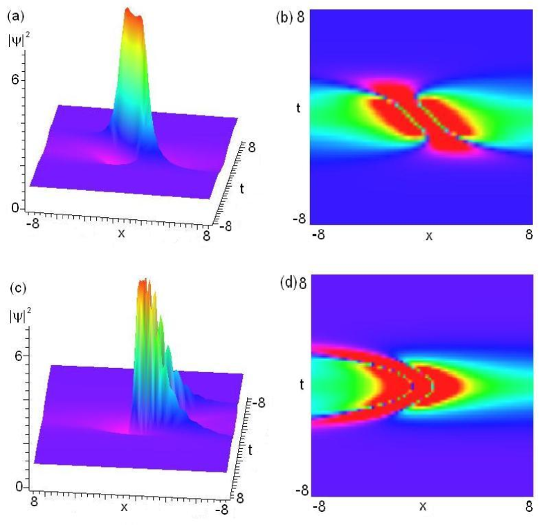
Figure 1: (color online). Wave propagations (left column) and contour plots (right column) for the intensity $|\psi_{1}|^{2}$ (15) of the first-order rational-like solution (14) for $\alpha=\alpha_{0}=1.0,\ \beta=0.5t^{2},\ \gamma(t)=0.1\tanh(t){\rm sech}(t)$. (a)-(b) $\delta(t)=t$; (c)-(d) $\delta(t)=t^{2}$.

For the fixed parameters $\alpha_{0}=1,\ \chi_{0}(t)=0$ and $\gamma(t)=0.1\tanh(t){\rm sech}(t)$, i) if we choose other free functions as the polynomials of time $t$, i.e. $\alpha(t)=1,\ \beta(t)=0.5t^{2}$, then Figures 1a and 1b depict the dynamical behavior of the rational-like solution (14) for different terms $\delta(t)=t,\ t^{2}$, respectively, in which the other coefficients $g(t)$ and $v(x,t)$ in Eq. (2) are given by

$$g(t)=\frac{1}{4}t^{2}e^{[{\rm sech}(t)-1]/5},$$ (16a)

$$v(x,t)=4t^{-3}x+t^{-2}\ \ \ {\rm for}\ \ \ \delta(t)=t,$$ (16b)

$$v(x,t)=4t^{-2}x+4\ \ \ {\rm for}\ \ \ \delta(t)=t^{2};\qquad\qquad\qquad\qquad\qquad\qquad\qquad\qquad\qquad\qquad$$ (16c)

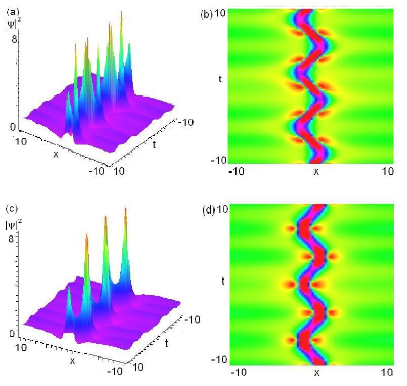
Figure 2: (color online). Wave propagations (left column) and contour plots (right column) for the intensity $|\psi_{1}|^{2}$ (15) of the first-order rational-like solution (14) for $\alpha_{0}=1.0,\ \gamma(t)=0.1\tanh(t){\rm sech}(t),\ k=0.6,\ \alpha(t)={\rm dn}(t,k),\ \beta(t)={\rm cn}(t,k)$: (a)-(b) $\delta(t)={\rm sn}(t,k)$; (c)-(d) $\delta(t)={\rm cn}(t,k)$.

ii) if we choose other free functions as the periodic functions of time $t$, i.e. $\alpha(t)={\rm dn}(t,k),\ \beta(t)={\rm cn}(t,k)$, then Figures 2a and 2b display the dynamical behavior of the intensity of the rational-like solution (14) for different terms $\delta(t)={\rm sn}(t,k),\ {\rm cn}(t,k)$, respectively, in which the coefficients $g(t)$ and $v(x,t)$ in Eq. (2) are given by

$$g(t)=\frac{1}{2}\,{\rm cn}(t,k)\,{\rm dn}(t,k)e^{[{\rm sech}(t)-1]/5},$$ (17a)

$$v(x,t)=\frac{k^{2}{\rm cn}(t,k)}{2\,{\rm dn}^{2}(t,k)}x^{2}+\frac{1}{2}\,{\rm cn}(t,k)[k^{2}{\rm sd}(t,k)x-1]^{2}\ \ {\rm for}\ \ \delta(t)={\rm sn}(t,k),$$ (17b)

$$v(x,t)=\frac{k^{2}{\rm cn}(t,k)}{2\,{\rm dn}^{2}(t,k)}x^{2}+\frac{{\rm dn}(t,k)}{{\rm cn}^{2}(t,k)}x+\frac{1}{2}{\rm cn}(t,k)[k^{2}{\rm sd}(t,k)x+{\rm sc}(t,k)]^{2}\ \ {\rm for}\ \ \delta(t)={\rm cn}(t,k);$$ (17c)

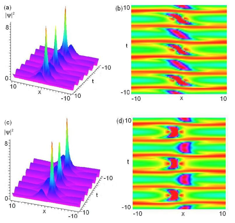
Figure 3: (color online). Wave propagations (left column) and contour plots (right column) for the intensity $|\psi_{1}|^{2}$ (15) of the first-order rational-like solution (14) for $\alpha_{0}=1.0,\ \gamma(t)=0.1\tanh(t){\rm sech}(t),\ k=0.6,\ \alpha(t)={\rm cn}(t,k),\ \beta(t)={\rm dn}(t,k)$: (a)-(b) $\delta(t)={\rm sn}(t,k)$; (c)-(d) $\delta(t)={\rm dn}(t,k)$.

iii) if we choose other free functions as the periodic functions of time $t$, i.e. $\alpha(t)={\rm cn}(t,k),\ \beta(t)={\rm dn}(t,k)$, then Figures 3a and 3b exhibit the dynamical behavior of the rational-like solution (14) for different terms $\delta(t)={\rm sn}(t,k),\ {\rm dn}(t,k)$, respectively, in which the coefficients $g(t)$ and $v(x,t)$ in Eq. (2) are given by

$$g(t)=\frac{1}{2}\,{\rm cn}(t,k)\,{\rm dn}(t,k)e^{[{\rm sech}(t)-1]/5},$$ (18a)

$$v(x,t)=\frac{{\rm dn}(t,k)}{2\,{\rm cn}^{2}(t,k)}x^{2}+\frac{1}{2}\,{\rm dn}(t,k)[{\rm sc}(t,k)x-1]^{2}\ \ {\rm for}\ \ \delta(t)={\rm sn}(t,k),$$ (18b)

$$v(x,t)=\frac{k^{2}{\rm dn}(t,k)}{2\,{\rm cn}^{2}(t,k)}x^{2}+\frac{k^{2}{\rm cn}(t,k)}{{\rm dn}^{2}(t,k)}x+\frac{1}{2}{\rm dn}(t,k)[{\rm sc}(t,k)x+k^{2}{\rm sd}(t,k)]^{2}\ \ {\rm for}\ \ \delta(t)={\rm dn}(t,k).$$ (18c)

It follows from these figures that the rational-like solution (14) is different from the known rational solution of the NLS equation (1) [16, 17, 22, 23, 24, 29, 30], and may be useful to raise the possibility of relative experiments and potential applications for the RW phenomenon.

Second-order rational-like solution— It follows from (13) that we have the second-order rational solution of Eq. (2) in the form $P(\eta,\tau)=\mathcal{P}_{2}(\eta,\tau)/[b\mathcal{A}_{2}(\eta,\tau)]$ and $Q(\eta,\tau)=\mathcal{Q}_{2}(\eta,\tau)/[c\mathcal{A}_{2}(\eta,\tau)]$, where

$$\begin{array}[]{l}\mathcal{P}_{2}(\eta(x,t),\tau(t))=\displaystyle-\frac{1}{2}\eta^{4}-6\eta^{2}\tau^{2}-10\tau^{4}-\frac{3}{2}\eta^{2}-9\tau^{2}+\frac{3}{8},\vspace{0.1in}\cr\mathcal{Q}_{2}(\eta(x,t),\tau(t))=\displaystyle-\tau\left[\eta^{4}+4\eta^{2}\tau^{2}+4\tau^{4}-3\eta^{2}+2\tau^{2}-\frac{15}{4}\right],\vspace{0.1in}\cr\mathcal{A}_{2}(\eta(x,t),\tau(t))=\displaystyle\frac{1}{12}\eta^{6}+\frac{1}{2}\eta^{4}\tau^{2}+\eta^{2}\tau^{4}+\frac{2}{3}\tau^{6}+\frac{1}{8}\eta^{4}+\frac{9}{2}\tau^{4}-\frac{3}{2}\eta^{2}\tau^{2}+\frac{9}{16}\eta^{2}+\frac{33}{8}\tau^{2}+\frac{3}{32},\end{array}$$ (22)

As a consequence, based on the transformations (4) and (9), we have the second-order rational-like solution (two-rogon solution) of Eq. (2)

$$\psi_{2}(x,t)=a_{0}\sqrt{|\alpha(t)|}\,e^{\int^{t}_{0}\gamma(s)ds}\left[1+\frac{\mathcal{P}_{2}(\eta(x,t),\tau(t))+i\mathcal{Q}_{2}(\eta(x,t),\tau(t))}{\mathcal{A}_{2}(\eta(x,t),\tau(t))}\right]e^{i[\chi(x,t)+\tau(t)]}\qquad\qquad$$ (23)

whose intensity is given by

$$|\psi_{2}(x,t)|^{2}=a_{0}^{2}|\alpha(t)|\,e^{2\int^{t}_{0}\gamma(s)ds}\frac{[\mathcal{A}_{2}(\eta(x,t),\tau(t))+\mathcal{P}_{2}(\eta(x,t),\tau(t))]^{2}+\mathcal{Q}_{2}^{2}(\eta(x,t),\tau(t))}{\mathcal{A}_{2}^{2}(\eta(x,t),\tau(t))},\quad$$ (24)

where $\eta(x,t)=\alpha(t)x+\delta(t)$, and $\chi(x,t),\ \tau(t)$ are given by Eqs. (11a) and (12). The obtained second-order rational-like solution (23) is also different from the known rational solutions of the NLS equation (1) [22, 29], since some free functions of time $t$ are involved. Similar to the first-order rational-like solution, the solution (23) can also reduce to the known one of Eq. (1) in Refs. [22, 29].

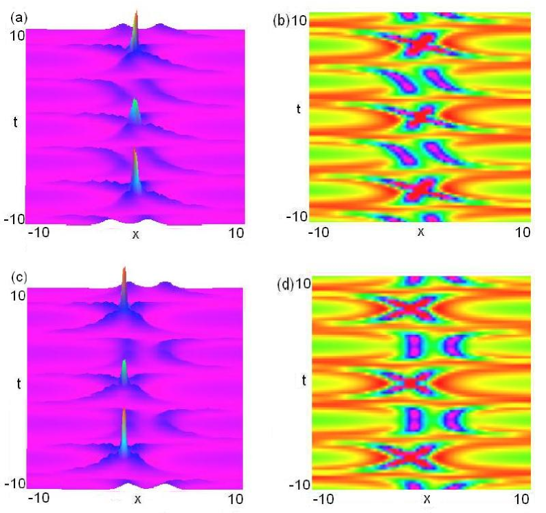
Figure 6: (color online). Wave propagations (left column) and contour plots (right column) for the intensity $|\psi_{2}|^{2}$ (24) of the second-order rational-like solution (23) for $\alpha_{0}=1.0,\ \gamma(t)=0.1\tanh(t){\rm sech}(t),\ k=0.6,\ \alpha(t)={\rm cn}(t,k),\ \beta(t)={\rm dn}(t,k)$: (a)-(b) $\delta(t)={\rm sn}(t,k)$; (c)-(d) $\delta(t)={\rm dn}(t,k)$.

For the fixed parameters $\alpha_{0}=1,\ \chi_{0}(t)=0,\ \gamma(t)=0.1\tanh(t){\rm sech}(t)$, i) if we choose other free functions as the polynomials of time $t$, i.e. $\alpha(t)=1,\ \beta(t)=0.5t^{2}$, then Figures 4a and 4b depict the dynamical interaction of the two-rogon solution (23) for different terms $\delta(t)=0.1t,\ t^{2}$; ii) if we choose the free functions as the periodic functions of time $t$, i.e. $\alpha(t)={\rm dn}(t,k),\ \beta(t)={\rm cn}(t,k)$, then Figures 5a and 5b illustrate the dynamical interaction of the two-rogon solution (23) for different terms $\delta(t)={\rm sn}(t,k),\ {\rm cn}(t,k)$; iii) if we take other free functions as the periodic functions of time $t$, i.e. $\alpha(t)={\rm cn}(t,k),\ \beta(t)={\rm dn}(t,k)$, then Figures 6a and 6b exhibit the dynamical interaction of the two-rogon solution (23) for different terms $\delta(t)={\rm sn}(t,k),\ {\rm dn}(t,k)$.

In conclusion, we have presented the analytical first-order and second-order rational-like solution pairs (nonautonomous rogons) of the inhomogeneous nonlinear Schrödinger equation with variable coefficients by using the similarity transformation and direct ansatz. By using the direct approach [29], we can also obtain the higher-order rational-like solutions of Eq. (2) which are omitted here. These obtained solutions be used to describe the possible formation mechanisms for the optical rogue wave phenomenon in optical fibres, the oceanic rogue wave phenomenon in the deep ocean, and the matter rogue wave phenomenon in Bose-Einstein condensates. Furthermore, it should be emphasized that we give the explicit solutions for the existence of matter rogons in Bose-Einstein condensates. Moreover, the snake propagation traces and the interaction of optical nonautonomous rogons are exhibited by choosing some free functions of time. Some shapes of the optical nonautonomous rogons and fascinating interactions between two optical nonautonomous rogons are also achieved with different functions. These solutions modify the known solutions related to the optical rogons. Moreover, this constructive idea can be also extended to other nonlinear systems with variable coefficients to generate nonautonomous rogons. This will further excite the study of rogons in the field of nonlinear science.

Acknowledgements

This work was supported by the FCT SFRH/BPD/41367/2007 and the NSFC60821002/F02.

  

List of the Figure Captions

1. Wave propagations (left column ) and contour plots (right column) for the intensity $|\psi_{1}|^{2}$ (15) of the first-order rational-like solution (14 for $\alpha=\alpha_{0}=1.0,\ \beta=0.5t^{2},\ \gamma(t)=0.1\tanh(t){\rm sech}(t)$. (a)-(b) $\delta(t)=t$; (c)-(d) $\delta(t)=t^{2}$.

2. Wave propagations (left column) and contour plots (right column) for the intensity $|\psi_{1}|^{2}$ (15) of the first-order rational-like solution (14) for $\alpha_{0}=1.0,\ \gamma(t)=0.1\tanh(t){\rm sech}(t),\ k=0.6,\ \alpha={\rm dn}(t,k),\ \beta(t)={\rm cn}(t,k)$: (a)-(b) $\delta(t)={\rm sn}(t,k)$; (c)-(d) $\delta(t)={\rm cn}(t,k)$.

3. Wave propagations (left column) and contour plots (right column) for the intensity $|\psi_{1}|^{2}$ (15) of the first-order rational-like solution (14) for $\alpha_{0}=1.0,\ \gamma(t)=0.1\tanh(t){\rm sech}(t),\ k=0.6,\ \alpha={\rm cn}(t,k),\ \beta(t)={\rm dn}(t,k)$: (a)-(b) $\delta(t)={\rm sn}(t,k)$; (c)-(d) $\delta(t)={\rm dn}(t,k)$.

4. Wave propagations (left column) and contour plots (right column) for the intensity $|\psi_{2}|^{2}$ (24)of the second-order rational-like solution (23) for $\alpha_{0}=1.0,\ \gamma(t)=0.1\tanh(t){\rm sech}(t),\ k=0.6,\ \alpha={\rm dn}(t,k),\ \beta(t)={\rm cn}(t,k)$: (a)-(b) $\delta(t)=0.1t$; (c)-(d) $\delta(t)=t^{2}$.

5. Wave propagations (left column) and contour plots (right column) for the intensity $|\psi_{2}|^{2}$ (24) of the second-order rational-like solution (23) for $\alpha_{0}=1.0,\ \gamma(t)=0.1\tanh(t){\rm sech}(t),\ k=0.6,\ \alpha={\rm dn}(t,k),\ \beta(t)={\rm cn}(t,k)$: (a)-(b) $\delta(t)={\rm sn}(t,k)$; (c)-(d) $\delta(t)={\rm cn}(t,k)$.

6. Wave propagations (left column) and contour plots (right column) for the intensity $|\psi_{2}|^{2}$ (24) of the second-order rational-like solution (23) for $\alpha_{0}=1.0,\ \gamma(t)=0.1\tanh(t){\rm sech}(t),\ k=0.6,\ \alpha={\rm cn}(t,k),\ \beta(t)={\rm dn}(t,k)$: (a)-(b) $\delta(t)={\rm sn}(t,k)$; (c)-(d) $\delta(t)={\rm dn}(t,k)$.

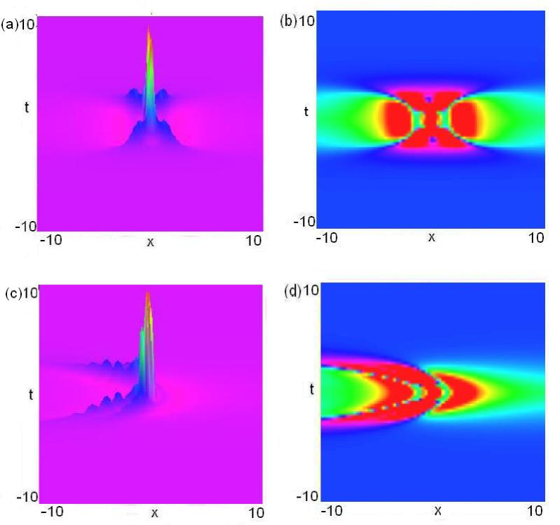
Figure 4: (color online). Wave propagations (left column) and contour plots (right column) for the intensity $|\psi_{2}|^{2}$ (24) of the second-order rational-like solution (23) for $\alpha=\alpha_{0}=1.0,\ \gamma(t)=0.1\tanh(t){\rm sech}(t),\ \beta(t)=0.5t^{2}$: (a)-(b) $\delta(t)=0.1t$; (c)-(d) $\delta(t)=t^{2}$.

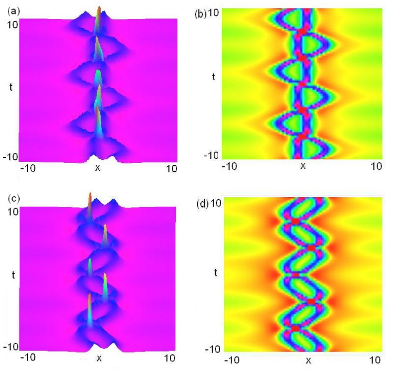
Figure 5: (color online). Wave propagations (left column) and contour plots (right column) for the intensity $|\psi_{2}|^{2}$ (24) of the second-order rational-like solution (23) for $\alpha_{0}=1.0,\ \gamma(t)=0.1\tanh(t){\rm sech}(t),\ k=0.6,\ \alpha(t)={\rm dn}(t,k),\ \beta(t)={\rm cn}(t,k)$: (a)-(b) $\delta(t)={\rm sn}(t,k)$; (c)-(d) $\delta(t)={\rm cn}(t,k)$.

References

[1]
[2] C. Sulem, P. L. Sulem, The Nonlinear Schrödinger Equation: Self-focusing and Wave
Collapse, Springer-Verlag, New York, 1999.
[3] Y. S. Kivshar, G. P. Agrawal, Optical Solitons: From Fibers to
Photonic Crystals, Academic, San Diego, 2003.
[4] A. Hasegawa, M. Matsumoto, Optical Solitons in Fibers, Springer, Berlin, 2003.
[5] C. J. Pethick, H. Smith, Bose-Einstein Condensation in
Dilute Gases, Cambridge University Press, Cambridge, 2002.
[6] F. Dalfovo, S. Giorgini, L.P. Pitaevskii, S. Stringari, Rev. Mod. Phys. 71 (1999) 463.
[7] R. Carretero-González, D. J. Frantzeskakis, P. G. Kevrekidis, Nonlinearity, 21 (2008)
R139.
[8] M. Onorato, A. R. Osborne, M. Serio, S. Bertone, Phys. Rev. Lett. 86 (2001)
5831.
[9] C. Kharif, E. Pelinovsky, Eur. J. Mech. B (Fluids) 22 (2003) 603.
[10] A. R. Osborne, Nonlinear Ocean Waves, Academic
Press, New York, 2009.
[11] C. Kharif, E. Pelinovsky, A. Slunyaev, Rogue
Waves in the Ocean, Observation, Theories and Modeling, Springer,
New York, 2009.
[12] L. Draper, Mar. Obs. 35 (1965) 193.
[13] P. Müller, Ch. Garrett, A. Osborne, Oceanography 18 (2005) 66.
[14] D. R. Solli, C. Ropers, P. Koonath, B. Jalali, Nature
450 (2007) 1054.
[15] D.-I. Yeom, B. Eggleton, Nature 450 (2007) 953.
[16] D. H. Peregrine, J. Aust. Math. Soc. Ser. B, Appl. Math.
25 (1983) 16.
[17] Y. C. Ma, Stud. Appl. Math. 60 (1979) 43.
[18] N. Akhmediev, V. I. Korneev, Theor. Math. Phys. 69 (1986) 1089.
[19] N. Akhmediev, V. M. Eleonskii, N. E. Kulagin, Theor. Math. Phys. 72 (1987) 809.
[20] K. B. Dysthe, K. Trulsen, Phys. Scr. T82 (1999) 48.
[21] V. V. Voronovich, V. I. Shrira, G. Thomas, J. Fluid Mech. 604 (2008) 263.
[22] N. Akhmediev, J. M. Soto-Crespo, A. Ankiewicz, Phys. Lett. A 373 (2009)
2137.
[23] N. Akhmediev, J. M. Soto-Crespo, A. Ankiewicz, Phys. Rev. A 80 (2009) 043818.
[24] A. Ankiewicz, N. Devine, N. Akhmediev, Phys. Lett. A 373 (2009) 3997.
[25] M. Onorato, A. R. Osborne, M. Serio, Phys. Rev. Lett. 96 (2006)
014503.
[26] P. K. Shukla, I. Kourakis, B. Eliasson, M. Marklund, L. Stenflo, Phys. Rev. Lett.
97 (2006) 094501.
[27] A. Grönlund, B. Eliasson, M. Marklund, Eur. Phys. Lett. 86
(2009) 24001.
[28] V. P. Ruban, Phys. Rev. Lett. 99 (2007) 044502.
[29] N. Akhmediev, J. M. Soto-Crespo, A. Ankiewicz, Phys. Rev.
E 80 (2009) 026601.
[30] N. Akhmediev, A. Ankiewicz, M. Taki, Phys. Lett. A 373 (2009) 675.
[31] M. Hopkin, Nature 430 (2004) 492.
[32] D. R. Solli, C. Ropers, B. Jalali, Phys. Rev.
Lett. 101 (2008) 233902.
[33] K. Hammani, C. Finot, J. M. Dudley, G. Millot1, Opt. Exp. 16 (2008)
16467.
[34] J. Kasparian, P. Béjot, J.-P. Wolf, J. M.
Dudley, Opt. Exp. 17 (2009) 12070.
[35] Yu. V. Bludov, V. V. Konotop, N. Akhmediev, Phys. Rev. A 80
(2009) 033610.
[36] B. A. Malomed, J. Opt. B 7 (2005) R53.
[37] S. Ponomarenko, G. P. Agrawal, Phys. Rev. Lett. 97 (2006) 13901.
[38] V. N. Serkin, A. Hasegawa, T. L. Belyaeva, Phys. Rev. Lett. 98 (2007) 074102.
[39] M. Centurion, M. A. Porter, P. G. Kevrekidis, D. Psaltis, Phys. Rev. Lett. 97 (2006)
033903.
[40] V. M. Pérez-Garcia, P. J. Torres, V. V. Konotop, Physica D 221 (2006) 31.
[41] J. Belmonte-Beitia, V. M. Pérez-Garcia, V. Vekslerchik, V. V. Konotop,
Phys. Rev. Lett. 98 (2008) 064102.
[42] Z. Y. Yan, Phys. Lett. A 361 (2007) 223.
[43] Z. Y. Yan, Phys. Scr. 75 (2007) 320.
[44] Z. Y. Yan, Constructive Theory and Applications of Complex
Nonlinear Waves, Science Press, Beijing, 2007.
[45] Z. Y. Yan, V. V. Konotop, Phys. Rev. E 80 (2009) 036607.
[46] N. J. Zabusky, M. D. Kruskal, Phys. Rev. Lett.
15 (1965) 240.
[47]