Analytical three-dimensional bright solitons and soliton-pairs in Bose-Einstein condensates with time-space modulation

Abstract

We provide analytical three-dimensional bright multi-soliton solutions to the (3+1)-dimensional Gross-Pitaevskii (GP) equation with time and space-dependent potential, time-dependent nonlinearity, and gain/loss. The zigzag propagation trace and the breathing behavior of solitons are observed. Different shapes of bright solitons and fascinating interactions between two solitons can be achieved with different parameters. The obtained results may raise the possibility of relative experiments and potential applications.

I Introduction

Solitons describe a class of fascinating nonlinear wave propagation phenomena appearing as a result of balance between nonlinearity and dispersion or diffraction properties of the medium under nonlinear excitations, which leads to undistorted propagation over extended distance Haus . One of the most important physically relevant realizations of solitons is provided by the matter-wave solitons in Bose-Einstein condensed atomic gas bec1 . Based on the successful experimental realization and theoretical analysis of Bose-Einstein condensations (BECs) in weakly interacting atomic gases bec1 , matter-wave dark solitons mws , vortices vor , bright solitons 3dsol , gap solitons gaps , and soliton chains chains have been observed and studied. These studies have stimulated a large amount of research activities, which enable the extension of linear atom optics to nonlinear atom optics bec2 .

The realization of higher-dimensional matter-wave solitons in BECs is still a challengeable topic because those solutions are usually unstable for (2+1)-D and (3+1)-D constant-coefficient nonlinear Schrödinger (NLS) equation due to the weak and strong collapse Sulem . However, different situations are observed in BECs with temporally or spatially modulated parameters. Alteration of atomic scattering length achieved by Feshbach resonance feshbach has been used to dynamically stabilize higher-dimensional bright solitons stab1 while periodic external potentials achieved by optical lattice has been used to generate and control higher-dimensional gap solitons stab2 . 1D periodic wave solutions are also predicted in BECs with time-space varying parameters 1DNLS . Moreover, the bright solitons 3bec and periodic wave solutions yanc were obtained in spinor BECs governed by a system of three coupled mean-field equations.

In this work, we present a detailed study on dynamics of analytical 3D bright matter-wave single solitons and soliton-pairs in BECs with time-space modulation. We note that 3D periodic wave solutions have been studied in the generalized NLS equation very recently belic ; yank . However, the authors did not study the soliton pair solutions and their interaction properties. By using the similarity 1DNLS ; yank ; simi and bilinear transformations bi , we can achieve different shapes of bright solitons and fascinating interactions between two solitons. In addition, the experimental possibilities for observability are discussed and the stability of solitons is illustrated numerically.

The paper is organized as follows. In the next section, the model under study is introduced. In Sec. III, the methods for solving the model equation are introduced. A relationship between the model and a practical system is established. In Sec. IV, we give the expressions of the bright solitons and the soliton-pairs. The interactions between two solitons are also investigated. In the last section, the case of the dark solitons is discussed and the outcomes are summarized.

II The GP model

The dynamics of a weakly interacting Bose gas at zero temperature is well described by the (3+1)-D GP model with time-space modulation bec1

$$\begin{array}[]{l}\displaystyle i\hbar\frac{\partial\Psi}{\partial t}\!=\!\left[-\frac{\hbar^{2}}{2m}\nabla^{2}\!+V_{\rm ext}(t,{\bf r})+G(t)|\Psi|^{2}\right]\!\!\Psi+i\,\Gamma(t)\Psi,\end{array}\vspace{-0.1in}$$ (2)

where $\nabla=(\partial_{x},\partial_{y},\partial_{z})$, ${\bf r}=(x,y,z)$, $\Psi\equiv\Psi(t,{\bf r})$ denotes the order parameter with $N=\int|\Psi|^{2}d{\bf r}$ being the number of atoms in the condensate, $G(t)=4\pi\hbar^{2}a_{s}(t)/m$ is the interaction function with $a_{s}(t)$ being the $s$-wave scattering length modulated by a Feshbach resonance, and $\Gamma(t)$ is the gain/loss term, which is phenomenologically incorporated to account for the interaction of atomic or thermal clouds. We note that the dissipative dynamics originating from the interaction between the radial and axial degrees of freedom has also been studied recently dissip . Here the potential is chosen as a harmonic trap $V_{\rm ext}(t,{\bf r})=(m/2)({\bf r}-{\bf e}(t))\omega^{2}(t)({\bf r}-{\bf e}(t))$ with $\omega(t)={\rm diag}(\omega_{x}(t),\omega_{y}(t),\omega_{z}(t))$ being a diagonal matrix of the trap frequencies in three directions and ${\bf e}(t)=$($e_{1}(t)$, $e_{2}(t)$, $e_{3}(t)$) corresponding to its center.

Using the suitably scales and variables: ${\bf r}=a_{z}{\bf r}^{\prime},\ t=\tilde{\omega}_{z}^{-1}t^{\prime},\ {\bf e}(t)=a_{z}{\bf e}^{\prime}(t)$, $\Psi=\sqrt{N/a_{z}^{3}}\psi$,  $a_{z}=[\hbar/(m\tilde{\omega}_{z})]^{1/2}$, and $\tilde{\omega}_{z}=\int\omega_{z}(t)dt$, we arrive at the dimensionless GP equation in the (3+1)-D space after dropping the primes

$$\begin{array}[]{l}\displaystyle i\frac{\partial\psi}{\partial t}=\left[-\frac{1}{2}\nabla^{2}+v(t,{\bf r})+g(t)|\psi|^{2}\right]\psi+i\,\gamma(t)\psi,\end{array}$$ (4)

where $g(t)=4\pi N^{2}a_{s}(t)/a_{z}^{4}$, $\gamma(t)=\Gamma(t)/(\hbar\tilde{\omega}_{z})$, and

$$\begin{array}[]{l}\displaystyle v(t,{\bf r})=\frac{1}{2}({\bf r}-{\bf e}(t)){\bf\alpha}^{2}(t)({\bf r}-{\bf e}(t))\end{array}$$ (6)

with $\alpha(t)={\rm diag}(\alpha_{1}(t),\alpha_{2}(t),\alpha_{3}(t))=\tilde{\omega}_{z}^{-1}\omega(t)$. Eq. (4) is associated with $\delta\mathcal{L}/\delta\psi^{*}=0$ in which the Lagrangian density can be written as

$$\begin{array}[]{l}\mathcal{L}=i(\psi\psi^{*}_{t}-\psi^{*}\psi_{t})+|\nabla\psi|^{2}-g(t)|\psi|^{4}\vspace{0.1in}\cr\qquad\quad-2[v(t,{\bf r})+i\gamma(t)]|\psi|^{2}.\end{array}$$ (9)

III Similarity solutions

Here we focus on the spatially localized bright solitons and soliton-paris for which $\lim_{|{\bf r}|\rightarrow\infty}\psi(t,{\bf r})=0$. Our first objective is to reduce Eq. (4) to the tractable NLS equation

$$\begin{array}[]{l}\displaystyle i\frac{\partial\Phi(\tau,\xi)}{\partial\tau}=-\frac{1}{2}\frac{\partial^{2}\Phi(\tau,\xi)}{\partial\xi^{2}}+\mathcal{G}|\Phi(\tau,\xi)|^{2}\Phi(\tau,\xi)\end{array}$$ (11)

using a proper similarity transformation, where $\tau\equiv\tau(t)$ and $\xi\equiv\xi(t,{\bf r})$ are both the unknown variables, and $\mathcal{G}$ is a constant. We explore the attractive nonlinearity, i.e. $\mathcal{G}=-1$, resulting in the bright multi-soliton solutions. The case $\mathcal{G}=1$ resulting in the dark multi-soliton solutions does not pose new challenges and will be discussed in the last section. Using the similarity transformation 1DNLS ; yank ; simi

$$\psi(t,{\bf r})=\rho(t)e^{i\varphi(t,{\bf r})}\Phi(\tau(t),\xi(t,{\bf r})),$$ (12)

and requiring $\Phi(\tau(t),\xi(t,{\bf r}))$ to satisfy Eq. (11) and $\psi(t,{\bf r})$ to be the solution of Eq. (4), we find a set of equations

$$\begin{array}[]{l}\nabla^{2}\xi=0,\ \ \xi_{t}+\nabla\xi\cdot\nabla\varphi=0,\ \ \tau_{t}=|\nabla\xi|^{2},\end{array}\quad$$ (13b)

$$\begin{array}[]{l}\displaystyle v(t,{\bf r})=-\frac{1}{2}|\nabla\varphi|^{2}-\varphi_{t},\ \ g(t)=\mathcal{G}\rho^{-2}|\nabla\xi|^{2},\end{array}\quad$$ (13d)

$$\begin{array}[]{l}\displaystyle\gamma(t)=\frac{1}{2}\nabla^{2}\varphi+\rho_{t}/\rho.\end{array}\quad$$ (13f)

Here for the harmonic trapping potential $v(t,{\bf r})$ given by Eq. (6), after some algebra it follows from system (13) that the similarity variables can be expressed as

$$\begin{array}[]{l}\displaystyle\xi(t,{\bf r})\!=\beta(t)\cdot{\bf r}\!+\!\int^{t}_{0}\beta(s)\cdot\sigma(s)ds,\vspace{0.1in}\cr\displaystyle\tau(t)\!=\int^{t}_{0}|\beta(s)|^{2}ds,\end{array}$$ (16)

where $\beta(t)=(\beta_{1}(t),\beta_{2}(t),\beta_{3}(t))$ denotes the vector of the inverse spatial widths of the localized solutions along $x,y,z$ directions, respectively, and $\sigma(t)=(\sigma_{1}(t),\sigma_{2}(t),\sigma_{3}(t))$ with $\sigma_{j}=\beta_{j}\int^{t}_{0}e_{j}\alpha_{j}^{2}\beta_{j}^{-1}dt$ relating to the velocity of the solitons. Moreover the nontrivial phase has the quadratic form

$$\begin{array}[]{l}\displaystyle\varphi(t,{\bf r})=-\frac{1}{2}{\bf r}A(t){\bf r}+\sigma\cdot{\bf r}-\frac{1}{2}\int^{t}_{0}({\bf e}\alpha^{2}{\bf e}+|\sigma|^{2})dt,\end{array}$$ (18)

where $A(t)={\rm diag}(\dot{\beta}_{1}/\beta_{1},\dot{\beta}_{2}/\beta_{2},\dot{\beta}_{3}/\beta_{3})$. The additional relations between $\alpha_{j}(t)$ and $\beta_{j}(t)=1/\nu_{j}(t)$ result in the Mathieu equations

$$\ddot{\nu}_{j}(t)+\alpha_{j}^{2}(t)\nu_{j}(t)=0,\quad(j=1,2,3).$$ (19)

Finally, the function $\rho(t)$ modulating the amplitude of solution $\psi$ and nonlinearity $g(t)$ can be also found by

$$\begin{array}[]{l}\rho(t)=\displaystyle\rho_{0}[\beta_{1}(t)\beta_{2}(t)\beta_{3}(t)]^{1/2}\exp\left[\int_{0}^{t}\gamma(s)ds\right],\vspace{0.1in}\cr g(t)=-\rho^{-2}(t)|\beta(t)|^{2},\end{array}$$ (22)

which depend on both $\beta_{j}(t)$ and gain/loss coefficient $\gamma(t)$ with $\rho_{0}$ being a non-zero parameter. Note that for the given $\beta_{j}(t)$, the nonlinearity $g(t)$ must attenuate (grow) exponentially in the gain (loss) medium $\gamma(t)>0\ (<0)$.

For the given $\alpha_{j}(t)$, one can, in principle, obtain corresponding $\beta_{j}(t)$ (or equivalently for the given $\beta_{j}(t)$ one can obtain $\alpha_{j}(t)$) based on Eq.(19). Furthermore, the bright $N$-soliton solutions of Eq.(11) can be obtained using the bilinear transformation bi : $\Phi_{N}=P^{(N)}(\tau,\xi)/Q^{(N)}(\tau,\xi)$. Here, $P^{(N)}$ and $Q^{(N)}$ satisfy $(iD_{\tau}+1/2D_{\xi}^{2})P^{(N)}\cdot Q^{(N)}=0$ and $D_{\xi}^{2}Q^{(N)}\cdot Q^{(N)}=2|P^{(N)}|^{2}$ with $D_{t}$ and $D_{\xi}$ being the bilinear operators and $P^{(N)}=\sum_{j=1}^{N}\epsilon^{2j-1}P_{2j-1}(\tau,\xi)$ and $Q^{(N)}=1+\sum_{j=1}^{N}\epsilon^{2j}Q_{2j}(\tau,\xi)$. Thus, by choosing $\beta_{j}(t)$ and $\gamma(t)$, we can generate $v(t,{\bf r})$ and $g(t)$ for which the generic bright $N$-soliton solutions of Eq. (4) can be found from Eq. (11) on the basis of Eq. (12). We will use this analytical result to construct the exact bright $N$-soliton solutions with many interesting nontrivial features.

For the convenience of analyzing different dynamical regimes described by the given model, we specify the magnitude of main physical parameters, which are feasible in experiments. We consider a condensed sodium sample trapped in the state $|3S_{1/2},F=1,m_{F}=-1\rangle$, which has the scattering length $a_{s}=2.75$ nm csys . The other parameters can be taken as $N=1.2\times 10^{6}$ and $\tilde{\omega}_{z}=(2\pi)\times 21$ Hz, which leads to $a_{z}=4.55$ $\mu$m and $\sqrt{N/a_{z}^{3}}=1.13\times 10^{2}$ $\mu$m^-3/2. To make sure the frequencies $\alpha_{j}(t)$ and nonlinearity $g(t)$ are bounded for realistic cases, we choose $\beta_{j}(t)$ and the gain/loss coefficient $\gamma(t)$ as the periodic functions

$$\beta(t)={\rm dn}(t,m){\bf b},\quad\gamma(t)=\gamma_{0}\,{\rm cn}(t,n),\ \ \ \gamma_{0}\in\mathbb{R}$$ (23)

where ${\bf b}=(b_{1},b_{2},b_{3})$ is a real constant vector describing the inverse of the width of the potential and the frequency, $m\in[0,\ 1)$ and $n\in[0,\ 1]$ are the modules of Jacobi elliptic functions. It is easy to see that $\gamma(t)=\gamma_{0}\,{\rm sech}(t)>0$ corresponds to the dissipative case when $n=1$ and $\gamma_{0}>0$ (we will focus on this condition next). In practical systems, the modulations of $\beta_{j}(t)$, $g(t)$ and $\gamma(t)$ depend on the use of the optical lattice and Feshbach-resonance techniques, i.e. we can achieve $\Gamma(t)$ and $a_{s}(t)$ by exerting particular time-dependent optical field and magnetic field.

It follows from Eqs. (19) and (23) that $\alpha_{j}(t)$ is given by

$$\alpha_{j}^{2}(t)=m^{2}\left[(2-m^{2})\,{\rm sd}^{2}(t,m)-{\rm nd}^{2}(t,m)\right].$$ (24)

Figure 1 shows the curves of $\alpha_{j}(t)$, $g(t)$, and $\gamma(t)$ vs $t$. For simplicity, we take $b_{j}=1$, i.e. $\alpha_{1}(t)=\alpha_{2}(t)=\alpha_{3}(t)$ corresponding to the isotropic potential, and consider that the center of the potential locates at the origin ($e_{j}=0$). We can also change $b_{j}$ to get an anisotropic potential and use nonzero $e_{j}$ to obtain moving bright solitons as those discussed in 1D case 1DNLS .

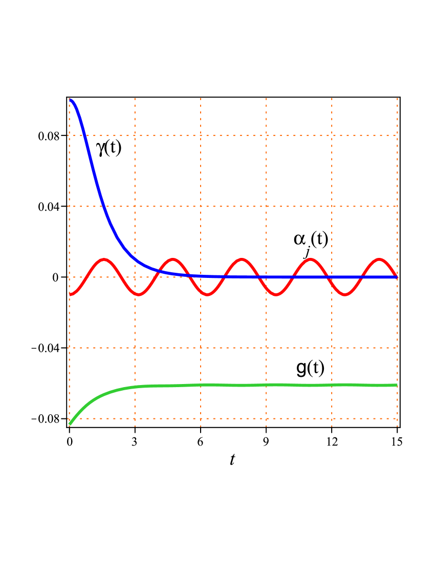
Figure 1: (color online). Curves of $\alpha_{j}(t)$, $g(t)$, and $\gamma(t)$ given by Eqs. (23) and (24) vs $t$ for $\rho_{0}=6.0$, $\gamma_{0}=m=0.1$, and $b_{j}=n=1.0$ ($j=1$, 2, 3).

IV Bright solitons and soliton pairs

Based on the discussions in the previous section, we arrive at the fundamental 3D time-varying bright solitons

$$\begin{array}[]{ll}\psi_{1}(t,{\bf r})\!=r_{1}\rho(t)\,{\rm sech}\big{[}r_{1}(\xi(t,{\bf r})\!-\!s_{1}\tau(t))\!-\!\ln|2r_{1}|\big{]}e^{i\theta},\vspace{-0.05in}\end{array}$$ (26)

where $\theta=s_{1}\xi(t,{\bf r})+(r_{1}^{2}-s_{1}^{2})/2\tau(t)+\varphi(t,{\bf r})$ with $r_{1},s_{1}\in\mathbb{R}$, and $\rho(t)$, $\varphi(t,{\bf r})$, $\xi(t,{\bf r})$, and $\tau(t)$ are given by Eqs. (16), (18) and (22).

Figure 2 exhibits the dynamics of the time-varying bright soliton (26). A breathing behavior is also evident, which can be managed by $\beta_{j}(t)$, $\gamma_{j}(t)$, and $\rho(t)$. For the case $m=0$, we have $\beta_{j}=b_{j}$ and $\alpha_{j}=0$, in which the travelling-wave bright soliton is obtained. In experiments, it can be simply realized for the zero linear potential. The bright soliton propagates in a zigzag trace for $m=0.1$ [see Fig.2(a)]. An important feature is that while $m\rightarrow 1$ ($\neq 1$) resulting in the larger period of $\beta_{j}(t)$ given by Eq.(23), the amplitude of the soliton close to the corners attenuates rapidly so that a soliton chain is generated [see Fig.2(b)]. In experiments, it can be realized by taking $\omega_{x}=\omega_{y}=\omega_{z}=m[(2-m^{2}){\rm sd}^{2}(t,m)-{\rm nd}^{2}(t,m)]^{1/2}\tilde{\omega}_{z}$.

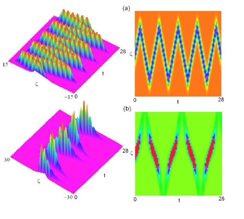
Figure 2: (color online). Propagations (left) and contour plots (right) of density for the bright soliton (26) in $(t,\,\zeta\equiv{\bf b}\cdot{\bf r})$-space for $r_{1}=0.5,\ s_{1}=\rho_{0}=2.0$, and $\gamma_{0}=0.01$. The others are the same as Fig.1. (a) The breathing bright soliton propagating in a zigzag trace for $m=0.1$. In the given sodium sample, the maximum density and width of the soliton are about $1.28$ $\mu$m^-3 and $12.13$ $\mu$m. The period is about $53.1$ ms. (b) The bright soliton chain for $m=0.9$. The maximum density and width of the soliton are about $1.28$ $\mu$m^-3 and $9.1$ $\mu$m. The period is about $91.0$ ms.

The interaction of the bright solitons plays an important role in the study of BECs. Here, we will also study the interaction between two bright solitons. The analytical 3D time-varying bright soliton pairs read

$$\begin{array}[]{l}\psi_{2}(t,{\bf r})=\rho(t)e^{i\varphi(t,{\bf r})}P(t,{\bf r})/Q(t,{\bf r}),\end{array}$$ (28)

where $P(t,{\bf r})$ and $Q(t,{\bf r})$ can be expressed as the series of exponential functions of $(t,{\bf r})$

$$\begin{array}[]{l}\displaystyle P(t,{\bf r})=\sum_{j=1}^{2}\delta_{j}e^{\eta_{j}}+\sum_{j,k=1,j\not=k}^{2}\lambda_{jk}e^{\eta_{j}+\eta_{j}^{*}+\eta_{k}},\vspace{0.1in}\cr\displaystyle Q(t,{\bf r})=1+\sum_{j,k=1}^{2}\Lambda_{jk}e^{\eta_{j}+\eta_{k}^{*}}+\Omega e^{\eta_{1}+\eta_{2}+\eta_{1}^{*}+\eta_{2}^{*}},\end{array}$$ (31)

with $\eta_{j}=\mu_{j}\xi(t,{\bf r})+\frac{i}{2}\mu_{j}^{2}\tau(t),\ \mu_{j}=r_{j}+is_{j}\ (r_{j},s_{j},\delta_{j}\in\mathbb{R})$, $\Lambda_{jk}=\delta_{j}\delta_{k}^{*}(\mu_{j}+\mu_{k}^{*})^{-2},\ \lambda_{jk}=(\mu_{k}-\mu_{j})\big{[}\delta_{k}\Lambda_{jk}(\mu_{k}+\mu_{k}^{*})^{-1}-\delta_{j}\Lambda_{kk}(\mu_{j}+\mu_{k}^{*})^{-1}\big{]}\ (j\not=k)$, and $\Omega=(|\delta_{1}\delta_{2}|)^{-1}|\mu_{1}-\mu_{2}|^{2}\big{(}\Lambda_{11}\Lambda_{22}\sqrt{\Lambda_{12}\Lambda_{21}}-\Lambda_{12}\Lambda_{21}\sqrt{\Lambda_{11}\Lambda_{22}}\big{)}$.

The dynamics of the 3D time-varying bright two-soliton solutions (28) is exhibited in Figure 3. Under the different parameters, we exhibit three cases for two weak zigzag solitons without interaction [see Fig.3(a)], two strong zigzag solitons with interaction [see Fig.3(b)], and strong-weak zigzag solitons with interaction [see Fig.3(c)]. Notice that similar with the bright solitons shown in Fig.2(b), for the case $m\rightarrow 1$ ($m\neq 1$), the amplitudes of the soliton-pairs close to the corners will almost decrease to zero so that panel (a) will degenerate to two parallel soliton chains while panels (b) and (c) will degenerate to the $><$-shaped soliton chains. The experimental realization of the dynamics regimes for the two-soliton solutions is similar with that for the bright one-soliton solutions.

We stress that the important feature that distinguishes our solutions from the reported in the literature mws ; vor ; 3dsol ; chains is the appearance of the time- and space-dependent functions in both the phase and the amplitude and which strongly affect the form and the behavior of bright solitons and their interactions.

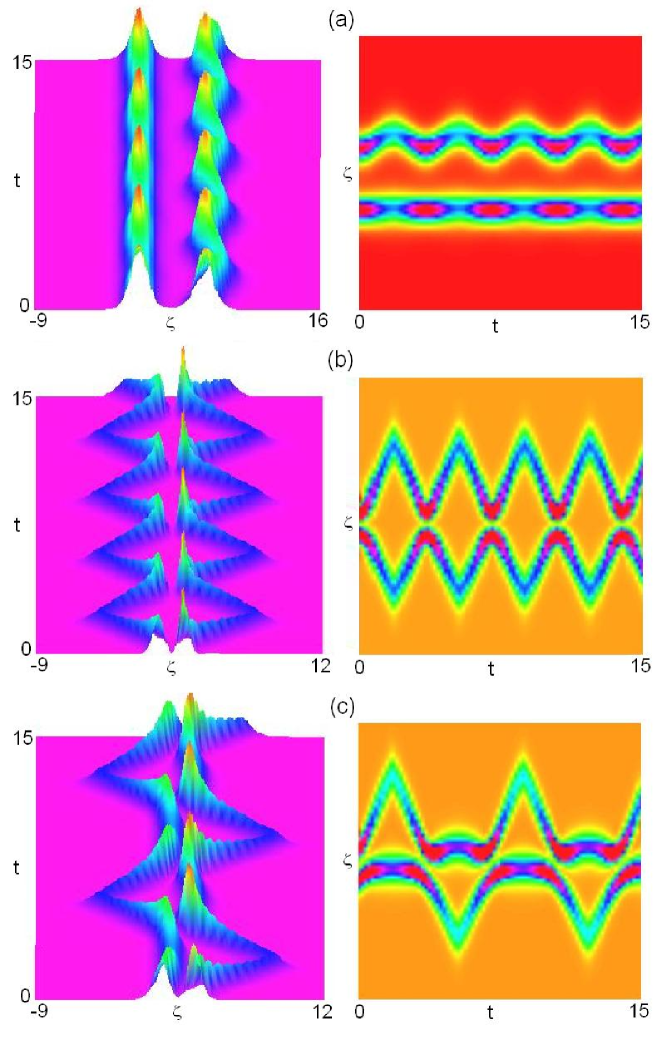
Figure 3: (color online). Propagations (left ) and contour plots (right) for collisions between bright two solitons (28) in $(t,\,\zeta\equiv{\bf b}\cdot{\bf r})$-space for $\gamma_{0}=0.01,\ \delta_{1,2}=\rho_{0}=1.0$, and $m=0.6$. The others are the same as Fig.1. (a) Two zigzag solitons without interaction for $r_{1}=1.0,\ r_{2}=1.2$ and $s_{1,2}=0$. In the given sodium sample, the maximum density and width of the left (right) soliton are about $1.8$ $\mu$m^-3 and $7.6$ $\mu$m ($1.5$ $\mu$m^-3 and $9.1$ $\mu$m). (b) Two strong zigzag solitons with interaction for $r_{1,2}=s_{1}=-s_{2}=1.2$. The maximum density and width of the left (right) soliton are about $6.2$ $\mu$m^-3 and $3.0$ $\mu$m ($17.5$ $\mu$m^-3 and $2.4$ $\mu$m) (c) Two strong-weak zigzag solitons with interaction for $r_{1}=1.2,\ r_{2}=1.5,\ s_{1}=1.05$ and $s_{2}=0$. The maximum density and width of the left (right) soliton are about $6.2$ $\mu$m^-3 and $4.2$ $\mu$m ($13.1$ $\mu$m^-3 and $3.8$ $\mu$m). The period of the zigzag oscillation is about $26.5$ ms in all panels.

In order to check the stability of the time-varying bright soliton (26), we make numerical simulations of Eq. (4) with the initial conditions given by Eq. (26) and different values of $m$. We find that the bright solitons are very stable for $m$ being small (e.g. $m=0.1$) [see Fig.4(a)]. With the increase of $m$, the bright solitons become unstable [see Fig.4(b)]. This is because large $m$ results in stronger oscillations of $\beta_{j}(t)$, which affect the coefficients of Eq. (4) and the behavior of the solutions.

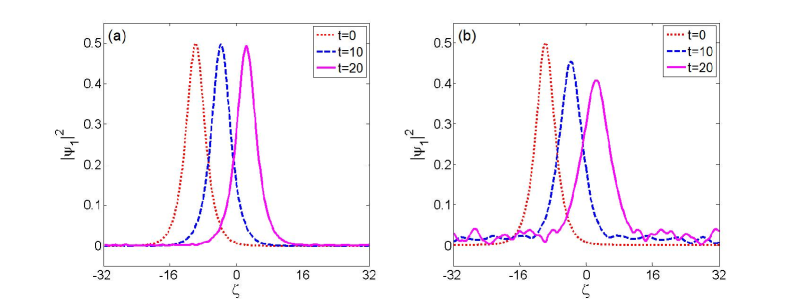
Figure 4: (color online). Numerical simulations of bright soliton from Fig. 2 vs $\zeta$ at $t=0$, 10, and 20. The initial conditions are given by Eq. (26) with $s_{1}=0.1$, $m=0.1$ in panel (a) and $m=0.9$ in panel (b). The other parameters are the same as those used in Fig. 2.

V Discussions and Conclusions

For completeness, we consider the repulsive nonlinearity in Eq. (11), i.e. $\mathcal{G}=-1$. In this case, the equation admits 3D dark soliton solutions in the form with a nontrial phase

$$\psi(t,{\bf r})=\big{\{}iv+k\tanh[k(\xi(t,{\bf r})-v\tau(t))]\big{\}}e^{-i\mu\tau(t)},$$ (32)

where $\mu$ is the chemical potential, $v=\sqrt{\mu-k^{2}}$, and $k$ is a free parameter satisfying $k^{2}<\mu$.

In summary, we have analytically constructed the novel 3D time-varying bright multi-soliton solutions for the (3+1)-D GP equation with time-space modulation. We focus on the bounded potential, nonlinearity, and gain/loss case to analyze the dynamics of the breathing and the zigzag propagation trace of the obtained solitons. Different shapes of the one-soliton solutions and the fascinating interactions between soliton-pairs were achieved. The stability of bright solitons have been checked numerically. The method we present here can be extended to study the higher-dimensional bright soliton solutions of other nonlinear systems and their various interaction properties. The model (4) can also be extended to describe 3D nonlinear optical media with varying coefficients belic after the transformation $z\leftrightarrow t$. The results we obtained may raise the possibility of relative experiments and potential applications.

- (1) H. A. Haus and W. S. Wong, Rev. Mod. Phys. 68, 423 (1996); M. A. Ablowitz and P. A. Clarkson, Solitons, Nonlinear Evolution Equations and Inverse Scattering (Cambridge University Press, Cambridge, 1991).
- (2) F. Dalfovo, S. Giorgini, L. P. Pitaevskii, and S. Stringari, Rev. Mod. Phys. 71, 463 (1999).
- (3) J. Denschlag, J. E. Simsarian, D. L. Feder, C. W. Clark, L. A. Collins, J. Cubizolles, L. Deng, E. W. Hagley, K. Helmerson, W. P. Reinhardt, S. L. Rolston, B. I. Schneider, W. D. Phillips, Science, 287 97 (2000); S. Burger, K. Bongs, S. Dettmer, W. Ertmer, K. Sengstock, A. Sanpera, G. V. Shlyapnikov, and M. Lewenstein, Phys. Rev. Lett. 83, 5198 (1999).
- (4) M. R. Matthews, B. P. Anderson, P. C. Haljan, D. S. Hall, C. E. Wieman, and E. A. Cornell, Phys. Rev. Lett. 83, 2498 (1999); K. W. Madison, F. Chevy, W. Wohlleben, and J. Dalibard, Phys. Rev. Lett. 84, 806 (2000).
- (5) L. Khaykovich, F. Schreck, G. Ferrari, T. Bourdel, J. Cubizolles, L. D. Carr, Y. Castin, C. Salomon, Science 296, 1290 (2002); S. L. Cornish, S. T. Thompson, and C. E. Wieman, Phys. Rev. Lett. 96, 170401 (2006).
- (6) K. E. Strecker, G. B. Partridge, A. G. Truscott, and R. G. Hulet, Nature 417, 150 (2002).
- (7) O. Zobay, S. Pötting, P. Meystre, and E. M. Wright, Phys. Rev. A 59, 643 (1999); A. Trombettoni and A. Smerzi, Phys. Rev. Lett. 86, 2353 (2001); B. Eiermann, Th. Anker, M. Albiez, M. Taglieber, P. Treutlein, K.-P. Marzlin, and M. K. Oberthaler Phys. Rev. Lett. 92, 230401 (2004); F. K. Abdullaev and M. Salerno, Phys. Rev. A 72, 033617 (2005).
- (8) W. M. Liu, B. Wu, and Q. Niu, Phys. Rev. Lett. 84, 2294 (2000); M. Trippenbach, Y. B. Band, and P. S. Julienne, Phys. Rev. A 62, 023608 (2000); I. Bloch, M. Köhl, M. Greiner, T. W. Hänsch, and T. Esslinger, Phys. Rev. Lett. 87, 030401 (2001).
- (9) C. Sulem and P. Sulem, The Nonlinear Schrödinger Equation: Self-focusing and Wave Collapse (Springer, Berlin, 1999).
- (10) J. Stenger, S. Inouye, M. R. Andrews, H.-J. Miesner, D. M. Stamper-Kurn, and W. Ketterle, Phys. Rev. Lett. 82, 2422 (1999); S. L. Cornish, N. R. Claussen, J. L. Roberts, E. A. Cornell, and C. E. Wieman, Phys. Rev. Lett. 85, 1795 (2000); J. L. Roberts, N. R. Claussen, S. L. Cornish, E. A. Donley, E. A. Cornell, and C. E. Wieman, Phys. Rev. Lett. 86, 4211 (2001).
- (11) H. Saito and M. Ueda, Phys. Rev. Lett. 90, 040403 (2003); F. K. Abdullaev, J. G. Caputo, R. A. Kraenkel, and B. A. Malomed, Phys. Rev. A 67, 013605 (2003); M. Matuszewski, E. Infeld, B. A. Malomed, and M. Trippenbach, Phys. Rev. Lett. 95, 050403 (2005).
- (12) P. J. Louis, E. A. Ostrovskaya, C. M. Savage, and Y. S. Kivshar, Phys. Rev. A, 67, 013602 (2003); B. B. Baizakov, B. A. Malomed, and M. Salerno, Phys. Rev. A 70, 053613 (2004).
- (13) V. M. Pérez-García, P. Torres, and V. V. Konotop, Physica D, 221, 31 (2006); J. Belmonte-Beiti, V. M. Pérez-García, and V. Vekslerchik, Phys. Rev. Lett.98, 064102 (2007); J. Belmonte-Beitia, V. M. Pérez-García, V. Vekslerchik, and V. V. Konotop, Phys. Rev. Lett. 100, 164102 (2008); A. T. Avelar, D. Bazeia, and W. B. Cardoso, Phys. Rev. E 79, 025602 (2009).
- (14) J. Ieda, T. Miyakawa, and M. Wadati, Phys. Rev. Lett. 93, 194102 (2004).
- (15) Z. Y. Yan, K. W. Chow, and B. A. Malomed, Chaos, Solitons and Fractals, 42, 3013 (2009).
- (16) M. Belić, N. Petrovic, W. Zhong, R. Xie, and G. Chen, Phys. Rev. Lett. 101, 123904 (2008).
- (17) Z. Y. Yan and V. V. Konotop, Phys. Rev. E 80, 036607 (2009).
- (18) Z. Y. Yan, Phys. Lett. A 361, 223 (2007); Z. Y. Yan, Phys. Scr. 75, 320 (2007).
- (19) R. Hirota, The Direct Method in Soliton Theory (Cambridge University Press, Cambridge, 2004).
- (20) A. Muryshev, G. V. Shlyapnikov, W. Ertmer, K. Sengstock, and M. Lewenstein, Phys. Rev. Lett. 89, 110401 (2002).
- (21) E. Tiesinga, C. J. Williams, P. S. Julienne, K. M. Jones, P. D. Lett, and W. D. Phillips, J. Res. Natl. Inst. Stand. Techol. 101, 505 (1996).