Sustaining star formation rates in spiral galaxies
Supernova-driven turbulent accretion disk models applied to THINGS galaxies

Abstract

Gas disks of spiral galaxies can be described as clumpy accretion disks without a coupling of viscosity to the actual thermal state of the gas. The model description of a turbulent disk consisting of emerging and spreading clumps (Vollmer & Beckert, 2003) contains free parameters, which can be constrained by observations of molecular gas, atomic gas and the star formation rate for individual galaxies. Radial profiles of 18 nearby spiral galaxies from THINGS, HERACLES, SINGS, and GALEX data are used to compare the observed star formation efficiency, molecular fraction, and velocity dispersion to the model. The observed radially decreasing velocity dispersion can be reproduced by the model. In the framework of this model the decrease in the inner disk is due to the stellar mass distribution which dominates the gravitational potential. Introducing a radial break in the star formation efficiency into the model improves the fits significantly. This change in star formation regime is realized by replacing the free fall time in the prescription of the star formation rate with the molecule formation timescale. Depending on the star formation prescription, the break radius is located near the transition region between the molecular-gas-dominated and atomic-gas-dominated parts of the galactic disk or closer to the optical radius. It is found that only less massive galaxies ($\log M({\rm M}_{\odot})\lower 2.15277pt\hbox{$\;\buildrel<\over{\sim}\;$}10)$) can balance gas loss via star formation by radial gas accretion within the disk. These galaxies can thus access their gas reservoirs with large angular momentum. On the other hand, the star formation of massive galaxies is determined by the external gas mass accretion rate from a putative spherical halo of ionized gas or from satellite accretion. In the absence of this external accretion, star formation slowly exhausts the gas within the optical disk within the star formation timescale.

1 Introduction

Gas accretion plays an important role for the evolution of galactic disks. The star formation rate in the solar neighborhood has been approximately constant over the last $\sim 10$ Gyr (Binney et al., 2000), while the local gas depletion time is $\approx 2$ Gyr (Evans, 2008). This suggests that the gas consumed by star formation must be replenished via external or internal accretion. Continuous addition of metal-poor gas would also explain the discrepancy between the observed stellar metallicity distribution in the solar neighborhood and that predicted by closed-box models of chemical evolution (Tinsley, 1981).

The need for accretion may also be seen from observations of other galaxies. Large spiral galaxies like the Milky Way typically have star formation rates of a few M_⊙/yr and gas reservoirs of order $10^{9}$ M_⊙ in the star-forming part of the galaxy. Over these regions, gas depletion times are 1–2 Gyr (Wong & Blitz, 2002), so that for these galaxies to survive in their present configuration, roughly the same amount of mass consumed by star formation must arrive at the galaxy center via some type of accretion. This accretion can be external, infalling gas from the galactic halo, or internal, radial gas transport via spiral arms and gas viscosity. In the absence of external accretion the spiral galaxy might deplete its gas and become a lenticular galaxy.

Turbulent galactic disks have been studied numerically and analytically in recent years. Wada & Norman (2007) used 3D, global hydrodynamic simulations of the central part of a late type galaxy to study the density distribution of the inhomogeneous ISM. They found that the density distribution is well fitted by a single lognormal function over a wide density range. Elmegreen (2002) first noticed that the Schmidt-Kennicutt law of the star formation rate can be reproduced if star formation occurs in dense gas above a critical density. The simulations of Wada & Norman (2007) did not include feedback from supernova (SN) explosions.

In a series of articles, Kim & Ostriker (2007), Shetty & Ostriker (2008), and Koyama & Ostriker (2009) studied the 2D evolution of an inhomogeneous ISM in a galactic disk without SN feedback.

Kim & Ostriker (2007) emphasize the importance of gravity due to gas and stars for driving interstellar turbulence. When strong feedback from SN is included (Shetty & Ostriker, 2008), the fraction of dense gas and thus star formation is reduced compared to the models of Kim & Ostriker (2007) and turbulence is driven by expanding shells in overdense regions. On the other hand, Agertz et al. (2009), who studied gaseous galactic disks by means of 3D, high-resolution hydrodynamical simulations with and without SN feedback, found that SN feedback is an important driver of turbulence in galaxies with star formation rates $\geq 10^{-3}$ M_⊙yr^-1kpc^-2. This star formation rate is found to galactic radii $\sim R_{25}$ in most of the nearby spiral galaxies investigated by Leroy et al. (2008).

Shetty & Ostriker (2008) note that the gas disk thickness is important for setting the index of the Schmidt-Kennicutt law. Koyama & Ostriker (2009) studied the relationships among pressure, vertical distribution of gas, and the fraction of dense gas in 2D hydrodynamic simulations of a starforming galactic disk with SN feedback. They found that vertical hydrostatic equilibrium gives a good estimate for the mean midplane pressure of the ISM. In their models they recover the observed ratio $R_{\rm mol}=M_{\rm H_{2}}/M_{\rm HI}$ if the gas surface density is proportional to the epicyclic frequency. Koyama & Ostriker (2009) state that the empirical result that $R_{\rm mol}$ is proportional to the mean midplane pressure of the ISM implies that the epicyclic frequency, the gas surface density, and the star formation rate per unit volume are interdependent, most probably due to a galaxy evolution with the Toomre parameter $Q$ close to unity. If gravitational instability of a clumpy and turbulent gas disk is taken into account, turbulence drives the disc to a regime of transition between instability at small scales and stability in the classical sense (Toomre $Q\sim 1$; Romeo et al. (2010)).

Most recently, Krumholz & Burkert (2010) have developed an analytical model for the evolution of a thin disk of gas and stars with an arbitrary rotation curve that is kept in a state of marginal gravitational instability ($Q\sim 1$) and energy equilibrium due to the balance between energy released by accretion and energy lost due to decay of turbulence. Equilibrium disks of this kind have been investigated by Vollmer & Beckert (2002). Krumholz & Burkert (2010) showed that disks initially out of equilibrium evolve into it on timescales comparable to the orbital period if the external gas accretion rate is high.

In this article we use the analytical models of Vollmer & Beckert (2003, hereafter VB03) to estimate the radial mass accretion rate of a sample of nearby spiral galaxies. The VB03 model treats galaxies as clumpy accretion disks using a simplified description of turbulence driven by supernova (SN) explosions. Because we focus on modeling the galactic disk within the optical radius, we neglect gravitational instabilities as energy source for turbulence (see Agertz et al., 2009). A gas disk without star formation might generate turbulence via gravitational instabilities, but once stars form, we assume that SN dominate energy injection. The formalism of our equilibrium model is close to that of Krumholz & Burkert (2010). The model naturally links the physical properties of the galactic gas disk (surface density, molecular fraction, star formation rate) to the midplane pressure which mainly depends on the stellar surface density, epicyclic frequency, the Toomre parameter, and the gas mass accretion rate (similar to Koyama & Ostriker, 2009). Furthermore, we assume the classical scale-independent Toomre stability criterion.

We compare these models to multiwavelength observations of 18 spiral galaxies from the THINGS sample (Walter et al., 2008) compiled by Leroy et al. (2008). From the comparison, we estimate the radial mass accretion rate of each galaxy.

The VB03 model considers the gas disk of a galaxy as a single turbulent medium. The dissipation timescale of turbulent kinetic energy on galactic scales is about the crossing time (Elmegreen, 2000), so that for a typical driving scale length of $\sim 100$ pc of the turbulent flow the dissipation time $\tau_{\rm d}\sim 10$ Myr . Therefore in order to maintain turbulence, an efficient, continuous, driving mechanism is needed. Possible candidates for such a driving mechanism are:

• gravitational instabilities like spiral arms (see, e.g. Gomez & Cox, 2002) or rotational shear (see, e.g., Wada & Norman, 2001; Vollmer & Beckert, 2002; Krumholz & Burkert, 2010),

• magneto-rotational instabilities (Balbus & Hawley, 1991),

• protostellar outflows (e.g., Wolf-Chase et al., 2000),

• stellar winds (e.g., Vink et al., 2000),

• UV radiation,

• supernova (SN) explosions (see e.g. Vollmer & Beckert, 2003; Agertz et al., 2009),

• external accretion (Elmegreen & Burkert, 2010; Klesse & Hennebelle, 2010).

Of these only SN explosions can balance the energy loss due to turbulent energy dissipation if the driving length scale is $\sim 100$ pc (Mac Low & Klessen, 2004) and the star formation rate is $\geq 10^{-3}$ M_⊙yr^-1kpc^-2 (Agertz et al., 2009). In cases where the driving length scale is of the order of the disk thickness ($\sim 500$ pc), the energy input due to gravitational instabilities can maintain turbulence in the interstellar medium (ISM) (Vollmer & Beckert, 2002; Krumholz & Burkert, 2010). The VB03 model and this paper consider only turbulence driven by SN.

In the VB03 model, SN-driven turbulence sets the disk structure and the disk structure determines the star formation rate, which in turn determines the SN rate. As a result, the conversion of gas into stars is of prime importance to the model. Despite a large variety of observations in different wavelengths, star formation in galaxies is not well understood (for recent reviews see Mac Low & Klessen, 2004; McKee & Ostriker, 2007). ISM turbulence in turn probably controls the star formation process to some degree (Mac Low & Klessen, 2004), but large scale gravitational instabilities (Toomre, 1964), thermal instabilities (Elmegreen & Parravano, 1994; Wolfire et al., 1995), and H₂ formation (Krumholz et al., 2009) may all be important.

In the last decades it was thought that star formation is controlled by the interplay between self-gravitation and magnetic fields. However, the interstellar medium (ISM) is of turbulent nature. Its structure is usually described as hierarchical (Scalo, 1985) over length scales of several magnitudes up to $\sim$100 pc. The neutral phase of the ISM is not uniform but has a fractal structure (Elmegreen & Falgarone, 1996).

Vollmer & Beckert (2003) developed an analytical model for clumpy accretion disks and included a simplified description of turbulence in the disk. In contrast to classical accretion disk theory (e.g., Pringle, 1981), VB03 do not use the “thermostat” mechanism, which implies a direct coupling between the heat produced by viscous friction and the viscosity itself, which is assumed to be proportional to the thermal sound speed. Thus, the viscosity, which is responsible for the gas heating, depends itself on the gas temperature. This leads to an equilibrium corresponding to a thermostat mechanism. Instead, VB03 use energy flux conservation, where the energy flux provided by SNe is transferred through a turbulent cascade to smaller scales where it is dissipated. The SN energy flux is expected to be proportional to the local star formation rate. In particular, the star formation recipe takes the turbulent nature of the ISM into account. VB03 showed that it is possible to reproduce the the local and global gas properties of the Galaxy with this model. It was, however, not possible at that time to compare observed radial profile to the VB03 model.

Here, we extend this comparison to a sample of 18 nearby spiral galaxies. Leroy et al. (2008) presented radial profiles of the star formation rate and gas surface density (CO and Hi) of these galaxies to study their star formation efficiencies. They showed that the SFE of H₂ alone is nearly constant (H₂ depletion time of $1.9$ Gyr) at their 800 pc resolution. Where the interstellar medium (ISM) is mostly Hi, however, the SFE decreases with increasing radius, a decline reasonably described by an exponential with scale length 0.2R₂₅–0.25R₂₅.

In this article we extend the formalism of VB03 (Sec. 2) by adding a break in the star formation rate (Sec. 2.1). Beyond this break the relevant timescale for star formation is no longer the free fall time of the most massive self-gravitating cloud at a given galactocentric radius, but the molecular formation timescale. In Sec. 4 and 5 the radial profiles presented in Leroy et al. (2008) are compared and discussed to the extended VB03 model. We discuss the implications of our findings in Sec. 6 and give our conclusions in Sec. 7.

2 The analytical model

Since the model is described in detail in VB03, we summarize here only the basic idea and the resulting expressions for the relevant disk properties.

The model considers the warm, cold, and molecular phases of the ISM as a single, turbulent gas. We assume this gas to be in vertical hydrostatic equilibrium, with the midplane pressure balancing the weight of the gas and stellar disk. The gas is taken to be clumpy, so that the local density is enhanced relative to the average density of the disk. Using this local density, we calculate two timescales relevant to star formation: the free fall of time of an individual clump and the characteristic timescale for H₂ to form on grains. The longer of these (modulo an empirical scaling factor) is taken as the governing timescale for star formation. The star formation rate is used to calculate the rate of energy injection by supernovae. This rate is related to the turbulent velocity dispersion (an observable) and the driving scale of turbulence. These quantities in turn provide estimates of the clumpiness of gas in the disk (i.e., the contrast between local and average density) and the rate at which viscosity moves matter inward.

The model relies on several empirical calibrations: e.g., the relationship between star formation rate and energy injected into the ISM by supernovae, the H₂ formation timescale (and its dependence on metallicity), and the turbulent dimension of the ISM (used to relate the driving length scale to the characteristic cloud size modulo a free parameter). As far as possible, these are drawn from observations of the Milky Way.

We are left with three free parameters. First, there is an unknown scaling factor relating the driving length of turbulence to the size of gravitationally bound clumps, which we call $\delta$. Second, the point at which the star formation timescale transitions from the free fall time to the H₂ formation time is a priori unknown. Third, the mass accretion rate, $\dot{M}$, which is related to the driving length and turbulent velocity, is a free parameter. In Section 4 via comparison to the present sample of galaxies, we constrain $\delta$. In practice, we also treat the Toomre $Q$ parameter of the gas as a “semi-free” parameter, allowing it to change somewhat from the observed value.

With these assumptions in hand, we may fit the model to a galaxy by comparing the observed kinematics, Hi, CO, and star formation rate profiles to those predicted by the model. The resulting fit yields the disk mass accretion rate and several other parameters that may be checked against expectations: the free fall time (or density) for the largest self-gravitating structures, the driving length of turbulence, and the approximate velocity of radial inflow.

In the remainder of this section, we discuss our assumptions in slightly more detail, justify them via comparison to observation and theory, and note the physics that we neglect.

ISM: Following, e.g., Mac Low & Klessen (2004), we view the ISM as a single turbulent gas. In this picture, the warm, cold, and molecular phases of the ISM are a single entity. Locally, the exact phase of the gas may depend on the local pressure, metallicity, stellar radiation field, stellar winds, and shocks. Here we view these factors as secondary, making a few simplifying assumptions. The equilibrium between the different phases of the ISM and the equilibrium between turbulence and star formation depends on three local timescales: the turbulent crossing time $t_{\rm turb}^{l}$, the molecule formation timescale $t_{\rm mol}^{l}$, and the local free fall timescale $t_{\rm ff}^{l}$ of a cloud.

Supernova-driven Turbulence: First, we assume that the gas is turbulent, so that the turbulent velocity is the relevant one throughout the disk (making the exact temperature of the gas is largely irrelevant). We assume that this turbulence is driven by SNe and that they input their energy in turbulent eddies that have a characteristic length scale, $l_{\rm driv}$, and a characteristic velocity, $v_{\rm turb}$. This driving length scale may be the characteristic length scale of a SN bubble, but it does not have to be so. It may be set by the interaction of multiple SN bubbles or of a SN with the surrounding ISM. We note that based on simulations, the assumption of a single driving scale may be a simplification (Joung & Mac Low, 2006). The VB03 model does not address the spatial inhomogeneity of the turbulent driving nor the mechanics of turbulent driving and dissipation. It is assumed that the energy input rate into the ISM due to SNe, $\dot{E}_{\rm SN}$, is cascaded to smaller scales without losses by turbulence. At scales smaller than the size of the largest selfgravitating clouds the energy is dissipated via cloud contraction and star formation. We refer to Mac Low & Klessen (2004) for a review of these topics. We limit our analytical model to the first energy sink which is the scale where the clouds become selfgravitating.

We can connect the energy input into the ISM by SNe directly to the star formation rate. With the assumption of a constant initial mass function (IMF) independent of environment one can write

$$\frac{\dot{E}_{\rm SN}}{\Delta A}=\xi\,\dot{\Sigma}_{*}=\xi\,\dot{\rho}_{*}l_{\rm driv}=\Sigma\nu\frac{v_{\rm turb}^{2}}{l_{\rm driv}^{2}}\ ,$$ (1)

where $\Delta A$ is the unit surface element of the disk. The factor of proportionality $\xi$ relates the local SN energy input to the local star formation rate and is assumed to be independent of local conditions. $\xi$ is normalized using Galactic observations by integrating over the Galactic disk and results in $\xi=4.6\times 10^{-8}$ (pc/yr)² (see VB03). The adopted energy that is injected into the ISM is $E^{\rm kin}_{\rm SN}=10^{50}$ ergs based on numerical studies by Thornton et al. (1998). The final two parts of Equation 1 assume that stars form over a characteristic scale equal to the driving length and equate energy output from SNe with the energy transported by turbulence (see VB03).

Star Formation in Molecular Clouds: Second, we assume that stars form out of gravitationally bound clouds. Where the timescale to form H₂ is short, we take the local gravitational free fall time, given by

$$t^{\rm l}_{\rm ff}=\sqrt{\frac{3\pi}{32G\rho_{\rm cl}}}\ ,$$ (2)

to be the relevant timescale for star formation. Here $G$ is the gravitational constant and $\rho_{\rm cl}$ the density of a single cloud.

Cloud collapse, and thus star formation can only proceed if enough molecules form during the cloud collapse to allow the gas to continue cooling. Therefore, where the timescale for H₂ formation is long (compared to the free fall time), we view this as the relevant timescale for star formation. We take the characteristic time to form H₂ out of H to be approximately

$$t_{\rm mol}^{l}=\alpha/\rho_{\rm cl}\ ,$$ (3)

where $\alpha$ is a coefficient that depends on metallicity and temperature (Draine & Bertoldi, 1996) and $\rho_{\rm cl}$ is the density of a single cloud. Unlike some other recent numerical and theoretical treatments of H₂ abundance by Robertson & Kravtsov (2008) and Krumholz et al. (2009), we take no account of the rate of destruction of H₂ via the UV radiation field. Instead, we assume H₂ to be destroyed via the collapse and subsequent star formation of a self-gravitating cloud.

The coefficient of the molecular formation timescale $\alpha$ is assumed to be metallicity dependent (Tielens & Hollenbach, 1985). Because we admit external gas accretion, the metallicity of the star-forming ISM mainly depends on the ratio of accretion to star formation rate $a$. Small $a<1$ lead to a metallicity derived from a closed box model, whereas in the case of $a>1$ the metallicity equals the true stellar yield $y_{\rm true}$ (Köppen & Edmunds, 1999). For gas fractions higher than 0.04 the difference between the two solutions is less than a factor of two. Moreover, Dalcanton (2007) showed that the effective yield $y_{\rm eff}=Z_{\rm gas}/\ln(1/f_{\rm gas})$, where $Z_{\rm gas}$ is the gas metallicity and $f_{\rm gas}$ the gas fraction, for disk galaxies with a rotation velocity higher than $100$ km s^-1 is approximately constant, i.e., for these galaxies a closed box model can be applied. We thus feel confident to estimate the metallicity based on a closed box model using the gas fraction :

$$\alpha=7.2\times 10^{7}\times\big{(}\log(\frac{\Sigma_{*}+\Sigma}{\Sigma})\big{)}^{-1}\ {\rm yr\,M_{\odot}pc^{-3}},$$ (4)

where $\Sigma_{*}$ is the stellar surface density and $\log$ refers to a natural logarithm. The calibration of the effective yield is based on the comparison of the observed O/H profiles with those of the closed box model (Sect. 4). Adopting a stellar and gas surface density of $\Sigma_{*}=40$ M_⊙pc^-2 and $\Sigma_{\rm gas}=10\,$ M_⊙pc^-2 at the solar radius of the Galaxy (Cox, 2000) yields $\alpha_{\odot}=4.5\times 10^{7}$ yr M_⊙pc^-3, which is twice the value used by Hollenbach & Tielens (1997).

This approach assumes that molecular clouds are relatively short lived, appearing and disappearing over roughly a free fall time (equivalently, by our construction, a turbulent crossing time); otherwise they might reach chemical equilibrium even when the H₂ formation time is long compared to the free fall time. Accordingly, we estimate the molecular fraction in the disk from the ratio of a cloud lifetime (i.e., the crossing or free-fall time) to the H₂ formation time scale: $f_{\rm mol}=\frac{\Sigma_{\rm H_{2}}}{\Sigma_{\rm HI}+\Sigma_{\rm H_{2}}}=t_{\rm turb}^{l}/t_{\rm mol}^{l}$.

Note that the molecular formation timescale, in particular, is fairly approximate — as noted above we have neglected radiation field and temperature dependences. Therefore we allow an extra factor $\gamma$ when comparing the two to derive the relevant timescale, with the transition between the two regimes at $t_{\rm ff}^{l}=\gamma t_{\rm mol}^{l}$. We derive a value of $\gamma=0.4\pm 0.3$ for the VB03 star formation prescription and $\gamma=0.12\pm 0.06$ for the star formation prescription following Krumholz & Tan (2007). comparing the model to the whole set of observations in Section 4.

Vertical Disk Structure: In the model, the disk scale height is determined unambiguously by the assumption of hydrostatic equilibrium and the turbulent pressure (Elmegreen, 1989):

$$p_{\rm turb}=\rho v_{\rm turb}^{2}=\frac{\pi}{2}G\Sigma(\Sigma+\Sigma_{*}\frac{v_{\rm turb}}{v_{\rm disp}^{*}})~{},$$ (5)

where $\rho$ is the average density, $v_{\rm turb}$ the gas turbulent velocity in the disk, $v_{\rm disp}^{*}$ the stellar vertical velocity dispersion, and $\Sigma$ the surface density of gas and stars. The stellar velocity dispersion is calculated by $v_{\rm disp}^{*}=\sqrt{2\pi G\Sigma_{*}H_{*}}$, where the stellar vertical height is taken to be $H_{*}=l_{*}/7.3$ with $l_{*}$ being the stellar radial scale length (Kregel et al., 2002). We neglect thermal, cosmic ray, and magnetic pressure. During the fitting procedure we realized that the local pressure equilibrium is of prime importance for the goodness of the fits.

Treatment as an Accretion Disk: The turbulent motion of clouds is expected to redistribute angular momentum in the gas disk like an effective viscosity would do. This allows accretion of gas towards the center and makes it possible to treat the disk as an accretion disk (e.g., Pringle, 1981). This gaseous turbulent accretion disk rotates in a given gravitational potential $\Phi$ with an angular velocity $\Omega=\sqrt{R^{-1}\frac{{\rm d}\Phi}{{\rm d}R}}$, where $R$ is the disk radius. The disk has an effective turbulent viscosity that is responsible for mass accretion and outward angular momentum transport. In this case, the turbulent velocity is driven by SN explosions, which stir the disk and lead to viscous transport of angular momentum. In addition, star formation removes gas from the viscous evolution. Following Lin & Pringle (1987), the evolution of the gas surface density is given by

$$\frac{\partial\Sigma}{\partial t}=-\frac{1}{R}\frac{\partial}{\partial R}\left(\frac{(\partial/\partial R)[\nu\Sigma R^{3}({\rm d}\Omega/{\rm}dR)]}{({\rm d}/{\rm d}R)(R^{2}\Omega)}\right)-\dot{\Sigma}_{*}+\dot{\Sigma}_{\rm ext}\ ,$$ (6)

where $\nu$ is the gas disk viscosity, $\Omega$ the angular velocity, and $\dot{\Sigma}_{\rm ext}$ is the external mass accretion rate. In contrast to Lin & Pringle (1987) we assume a continuous and non-zero external gas mass accretion rate. By approximating $\partial/\partial R\sim 1/R$, the global viscous evolution becomes

$$\frac{\partial\Sigma}{\partial t}\sim\frac{\Sigma\nu}{R^{2}}-\dot{\Sigma}_{*}+\dot{\Sigma}_{\rm ext}\ .$$ (7)

If the external and disk mass accretion rate keeps the combined Toomre parameter of the gas and stars smoothed over a few rotation periods to $Q_{\rm tot}\sim 1$, the gas surface density will only vary slowly with changes in the dark halo mass distribution (via $\Omega$) and the stellar disk structure, the gas loss due to star formation is balanced by external accretion as suggested by Fraternali & Binney (2008) and Marinacci et al. (2010), and the gas disk can be regarded as being stationary ($\partial\Sigma/\partial t=0$). Indeed, local spiral galaxies show a $Q_{\rm tot}$ not too far away from unity ($1.3$-$2.5$; Leroy et al. (2008)). For such a stationary gas disk, where star formation is balanced by external accretion, the local mass and momentum conservations yield:

$$\nu\Sigma=\frac{\dot{M}}{2\pi}\ ,$$ (8)

where $\dot{M}$ is the mass accretion rate within the disk. In the absence of external mass accretion, the gas disk can be assumed to be stationary as long as the star formation timescale $t_{*}$ exceeds the viscous timescale $t_{\nu}=R^{2}/\nu$. For $\dot{\Sigma}_{\rm ext}<\dot{\Sigma}_{*}$ and $t_{*}<t_{\nu}$ Eq. 8 is not valid. In this case the gas disk is rapidly turned into stars within the gas consumption time ($2$ Gyr, Evans (2008)). Since most spiral galaxies still have a significant amount of gas, we think that spiral galaxies are generally not in this state. Solving the time dependent Eq. 6 is beyond the scope of this work and we apply Eq. 8. Radial integration of Eq. 7 then gives

$$\frac{\partial M}{\partial t}\sim\dot{M}-\dot{M}_{*}+\dot{M}_{\rm ext}\ ,$$ (9)

where $M$ is the disk gas mass.

The viscosity is related to the driving length scale and characteristic velocity of the SN-driven turbulence by $\nu=v_{\rm turb}l_{\rm driv}$ (VB03). Because the lifetime of a collapsing and starforming cloud ($t_{\rm ff}^{l}<t_{\rm turb}^{l}$) is smaller than the turnover time of the large-scale eddy ($l_{\rm driv}/v_{\rm turb}$), the turbulent and clumpy ISM can be treated as one entity for the viscosity description.

Clumpiness: A critical factor in the model is the relationship between the density of individual clouds, $\rho_{\rm cl}$, and the average density of the disk, $\rho$. It is the density of individual clouds that is relevant to the timescale for star formation. In this model, the two are related by the volume filling factor, $\Phi_{\rm V}$ so that $\rho_{\rm cl}=\Phi_{\rm V}^{-1}\rho$.

Here $\rho_{\rm cl}$ refers to the density of the largest self-gravitating structures in the disk, so that for these structures the turbulent crossing time and gravitational free fall time are equal. The scale of such a cloud, $l_{\rm cl}$ is smaller than the driving length scale $l_{\rm driv}$ by a factor $\delta$, which we do not know a priori.

Shear due to differential galactic rotation could stabilize clouds, modifying the timescale for collapse. However, this effect is mainly important when the ratio of the cloud to disk surface density is lower than the ratio of cloud to disk velocity dispersion, which is not the case over most of the disk in a typical spiral. Typical GMC surface densities are $\sim 200$ M_⊙pc^-2 (Solomon et al., 1987), whereas disk surface densities only exceed $100$ M_⊙pc^-2 in the very center of spiral galaxies (Leroy et al., 2008). The ratio of velocity dispersion being about $0.5$, clouds at galactic radii larger than a few kpc are not stabilized by shear from galactic rotation.

We can calculate the turbulent timescale for the cloud, $t_{\rm turb}^{l}$, for a fractal ISM:

$$t_{\rm turb}^{l}=\delta^{-\frac{2}{3}-\frac{3-D}{3}}\,l_{\rm driv}/v_{\rm turb}\ ,$$ (10)

where $D$ is the fractal dimension (see, e.g., Frisch, 1995) of the ISM. We assume $D=2$ for a compressible, self-gravitating fluid, which is close to the findings of Elmegreen & Falgarone (1996). Once $\delta$ and thus $t_{\rm turb}^{l}$ are specified, we can solve for the density of the corresponding scale by setting $t_{\rm ff}^{l}=t_{\rm turb}^{l}$. The volume filling factor is then defined by comparing $\rho_{\rm cl}$ and $\rho$.

Because the relationship between the driving length scale, $l_{\rm driv}$ and $l_{\rm cl}$ is not known beforehand, we treat this as a free parameter. Once the volume filling factor is known (from $\delta$ or $l_{\rm cl}$), we can calculate the local star formation rate, $\dot{\rho_{*}}$, via

$$\dot{\rho}_{*}=\eta\frac{\rho}{t_{\rm sf}^{\rm l}}\ ,$$ (11)

where $t_{\rm sf}^{l}$ is the local timescale for star formation, either the free fall or molecular formation timescale, depending on local conditions. We assume $\eta=7\times 10^{-3}$ in consistency with Krumholz & Tan (2007). Since in our model the lifetime of a cloud is the free-fall as suggested by Ballesteros-Paredes & Hartmann (2007) or the molecule formation timescale, this implies that during the cloud lifetime about $1$ % of the cloud mass turns into stars.

In VB03 a different star formation prescription is used:

$$\dot{\rho}_{*}=\Phi_{\rm V}\frac{\rho}{t_{\rm sf}^{\rm l}}\ .$$ (12)

The vertically integrated star formation rate in the inner disk where $t_{\rm sf}^{\rm l}=t_{\rm ff}^{\rm l}=t_{\rm turb}^{\rm l}=\delta^{-1}t_{\rm turb}$ is

$$\dot{\Sigma}_{*}=\Phi_{\rm V}\frac{\rho}{t_{\rm ff}^{\rm l}}l_{\rm driv}=\delta\Phi_{\rm V}\rho v_{\rm turb}\ ,$$ (13)

i.e. it is the mass flux density of the turbulent ISM into the regions of star formation. This alternative description yields fitting results that are as good as those based on Eq. 11 (in practice $\eta\sim\Phi_{\rm V}\sim 10^{-2}$).

2.1 A Two Part Model

VB03 assumed that $t_{\rm sf}^{l}$ in Equation 11 is always the local free fall time. As described above, here we consider two regimes, adopting instead the H₂ formation time when this becomes long compared to $t_{\rm ff}^{l}$. Therefore, the present model has two parts. We label the first, where $t_{\rm sf}^{l}=t_{\rm ff}^{l}$ the inner disk. We label the second, where $t_{\rm sf}^{l}=t_{\rm mol}^{l}$ the outer disk. The change in regime should occur at the radius where $t_{\rm ff}^{l}=\gamma t_{\rm mol}^{l}$. Here $\gamma$ is a (free) scaling parameter that reflects a level of uncertainty in the application of the molecular formation timescale.

An alternative interpretation of the change in star formation regime is that (i) the star formation efficiency per free fall time or (ii) the volume or area filling factor of star forming regions change from the inner to the outer disk. The latter possibility is motivated by the work of Bush et al. (2008) who show that gaseous spiral arms formed in the inner disk region can propagate into the outer gas disk creating overdensities where stars can form. Since these gaseous arms occupy a smaller fraction of the disk area with increasing galactocentric radius, the azimuthally averaged surface and area filling factors decrease. Having this picture in mind, one can write for the outer disk

$$\dot{\rho}_{*}=\eta\frac{\rho}{t_{\rm mol}^{\rm l}}=\eta f_{\rm mol}\frac{\rho}{t_{\rm ff}^{\rm l}}=\tilde{\eta}\frac{\rho}{t_{\rm ff}^{\rm l}}$$ (14)

and

$$\dot{\rho}_{*}=\Phi_{\rm V}\frac{\rho}{t_{\rm mol}^{\rm l}}=\Phi_{\rm V}f_{\rm mol}\frac{\rho}{t_{\rm ff}^{\rm l}}=\tilde{\Phi}_{\rm V}\frac{\rho}{t_{\rm ff}^{\rm l}}\ .$$ (15)

In this formulation the relevant local star formation timescale is still the local free fall time of the clouds.

2.2 Model calculations

The VB03 model yields the following system of equations to describe a turbulent clumpy galactic accretion disk:

$$\nu=v_{\rm turb}l_{\rm driv}\ ,$$

$$\nu\Sigma=\frac{\dot{M}}{2\pi}\ ,$$

$$\Sigma=\rho\,H\ ,$$

$$p_{\rm turb}=\rho v_{\rm turb}^{2}=\frac{\pi}{2}G\Sigma(\Sigma+\Sigma_{*}\frac{v_{\rm turb}}{v_{\rm disp}^{*}})~{},$$

$$Q=\frac{v_{\rm turb}\Omega}{\pi G\Sigma}\ ,$$

$$\Sigma\nu\frac{v_{\rm turb}^{2}}{l_{\rm driv}^{2}}=\xi\,\dot{\Sigma}_{*}\ ,$$

$$\dot{\Sigma}_{*}=\Phi_{\rm V}\frac{\rho}{t_{\rm SF}^{\rm l}}l_{\rm driv}\ {\rm(VB03)\ or}\ =\eta\frac{\rho}{{t_{\rm SF}^{\rm l}}}l_{\rm driv}\ {\rm(KM05)}\ ,$$

$$t_{\rm SF}^{\rm l}=\sqrt{\frac{3\pi}{32G\rho_{\rm cl}}}\ {\rm or}\ =\frac{\alpha}{\rho_{\rm cl}}\ .$$

The meaning of the variables is given in Table 1. In the case of a selfgravitating gas disk ($\Sigma\gg\Sigma_{*}$) or a dominating stellar disk ($\Sigma_{*}\gg\Sigma$) the set of equations can be solved analytically (we use $\rho v_{\rm turb}^{2}=\pi G\Sigma^{2}$ and $\rho v_{\rm turb}^{2}=\pi G\Sigma\Sigma_{*}$). In Appendix A we give the equations relating several observables ($v_{\rm turb}$, $\Sigma$, $SFE=\dot{\Sigma_{*}}/\Sigma$, and $f_{\rm mol}$ and $f_{\rm mol}=\Sigma_{{\rm H}_{2}}/(\Sigma_{{\rm H}_{2}}+\Sigma_{{\rm HI}})$) and other quantities of interest ($l_{\rm driv}$, $\nu$, $\Phi_{V}$) to our free parameters ($\dot{M}$, $\delta$), assumed constants ($\xi$, $\eta$), the approximated metallicity ($\alpha$), the “fundamental” observables (stellar surface density $\Sigma_{*}$, radius $R$ and rotation $\Omega$), and the “quasi-free” parameter Toomre $Q$ of the gas (which we treat as free, but compare to observations).

For the global comparison between the observed and the model radial profiles we solve the set of equations given above numerically and we use

$$\frac{1}{t_{\rm SF}^{\rm l}}=\frac{1}{\sqrt{\frac{3\pi}{32G\rho_{\rm cl}}+\alpha^{2}/\rho_{\rm cl}^{2}}}\ .$$ (16)

3 Comparison with Observations

We compare the model described above to radial profiles of gas and star formation for 18 nearby spiral galaxies.

3.1 Data

The galaxies we compare to are all part of the THINGS (Walter et al., 2008) survey. To carry out the comparison, we use radial profiles of the Hi velocity dispersion measured via the second moment presented by Tamburro et al. (2009); rotation curves derived by de Blok et al. (2008); radial profiles of atomic (Hi) and molecular gas (traced via CO) surface density based on maps by Walter et al. (2008), Leroy et al. (2009), and Helfer et al. (2003); and profiles of star formation rate surface density derived by Leroy et al. (2008) from a combination of 24$\mu$m (SINGS, Kennicutt et al., 2003) and FUV (the GALEX NGA, Gil de Paz et al., 2007) intensity. We use stellar surface density estimates derived from SINGS $3.6\mu$m imaging by Leroy et al. (2008) assuming a constant mass-to-light ratio.

The profiles of atomic and molecular gas are combined into profiles of the molecular fraction, $f_{\rm mol}=\Sigma_{\rm H_{2}}/(\Sigma_{\rm H_{2}}+\Sigma_{\rm HI})$, and the profiles of star formation rate, Hi, and molecular gas are combined into profiles of star formation efficiency, $SFE=\dot{\Sigma}_{\rm*}/\Sigma$. Most of the profiles are drawn from Leroy et al. (2008) and details on methodology and data can be found there.

The following uncertainties affect the data in addition to the uncertainty in the mean value over the azimuthal ring estimated from the RMS scatter in that ring:

SFR and SFE: there is a $\sim 50\%$ uncertainty based on inter-comparison of different star formation rate tracers. Half of this ($\sim 0.1$ dex) is internal to the galaxy, the other half ($\sim 0.1$ dex) is galaxy-to-galaxy scatter (due to, e.g., the star formation history and dust properties).

Hi: THINGS is expected to recover the true Hi flux with 10% accuracy.

CO: The global CO-H₂ conversion factor is uncertain by a factor of 2, which dwarfs any uncertainty in the calibration. An additional systematic uncertainty is the dependence of the conversion factor on local conditions. The sample selection somewhat minimizes this concern. The CO data have been masked before constructing profiles, which can lead to artificially steep profiles at the edge of the CO emitting region.

Velocity dispersion: the scatter in the dispersion within a given ring is about 30%. Five of the 18 galaxies are too inclined to derive reliable velocity dispersions. Several regions have very high velocity dispersions, $>20$ km s^-1, which we expect are due at least partially to non-circular motions like bars, outflows, or streaming along spiral arms. We do not use these data in the comparison.

3.2 Procedure

The comparison is done in the following way:

1. The Toomre parameter of the gas is calculated using the observed Hi dispersion velocity $v_{\rm disp}$, rotation velocity $v_{\rm rot}$, and total gas surface density $\Sigma_{\rm gas}$:

   $$Q=\frac{v_{\rm disp}v_{\rm rot}}{\pi G\Sigma_{\rm gas}R}\ .$$ (17)

   This approximate form of $Q$ is used to avoid taking the (noisy) derivative of the observed rotation curve. In two cases, we adjust $Q$ somewhat from the measured value: (i) in the inner part ($R\leq 4$ kpc) of the disk of NGC 3351 where we set $Q=8$ and (ii) in the whole disk of NGC 2841 where we also assume $Q=8$. For both galaxies this corresponds to an approximately constant velocity dispersion of $\sim 12$-$15$ km s^-1. In cases without a measured velocity dispersion, we adopt a flat $Q$ (NGC 2841, NGC 3351), an exponentially declining $Q$ (NGC 3627), or a constant velocity dispersion of 15 km s^-1 (NGC 3521, NGC 7331).

2. We solve the set of equations given in Sect. 2.2 using a grid for values of $\delta$, $\dot{M}$, and $\gamma$. To account for the overall calibration uncertainties (Sect. 3.1), we calculate the models on the $\delta$-$\dot{M}$-$\gamma$-grid multiplying all points of $\Sigma_{\rm H_{2}}$ by $(0.63,1.,1.58)$, $v_{\rm turb}$ by $(0.79,1.,1.26)$, and $SFE$ by $(0.71,1.,1.41)$, allowing for all permutations. For each set of parameters the goodness $g$ of the fit is determined for each observable profile:

   $$g=\frac{1}{N}\sum_{i=1}^{N}\frac{(V^{\rm obs}_{i}-V^{\rm model}_{i})^{2}}{\sigma^{2}}\ ,$$ (18)

   where $N$ is the number of points of a radial profile, $V_{\rm obs/model}$ are the observed and the model points of the profiles, and $\sigma$ is the uncertainty of a point given by Leroy et al. (2008). At the end we calculate a total goodness of the fit by taking the mean of the goodnesses of the individual profiles. This does not correspond to a traditional $\chi^{2}$, because the uncertainties of the points of a given profile are correlated.

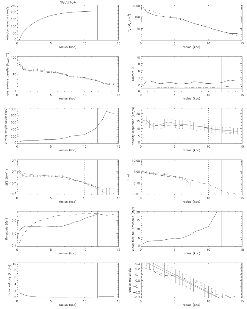
Figure 1: Comparison between modeled (KM05) and observed radial profiles. Form upper left to lower right: (i) Hi rotation curve, (ii) observed and fitted stellar surface density profile $\Sigma_{*}$ (the assumed $\Sigma_{*}$ for the fit is shown as a solid line), (iii) model (dashed) and observed (solid) total gas density profile $\Sigma$, (iv) Toomre $Q$ parameter of stars+gas (dash-dotted) and of the gas derived from observations (dotted) and assumed for the fit (solid), (v) driving scale length $l_{\rm driv}$, (vi) Hi velocity dispersion (solid) and model turbulent velocity dispersion (dashed), (vii) observed (solid) and modeled (dashed) star formation efficiency, (vii) observed (solid) and modeled (dashed) molecular fraction, (ix) star formation (solid) and viscous (dashed) timescales, (x) free fall timescale of the most massive selfgravitating gas clouds, (xi) radial velocity of the gas within the disk, and (xii) the observed (solid) and model (dashed) metallicity. The observed metallicity profiles is derived from $12+\log({\rm O/H})$ (Moustakas et al., 2010) assuming a solar oxygen abundance of $12+\log({\rm O/H})=8.9$. The two solid lines correspond to the calibrations of Kobulnicky & Kewley (2004) and Pilyugin & Thuan (2005) with an additional offset of 0.6 dex.

3. The final $\delta$ and $\dot{M}$ are determined by the mean of all $\delta$ and $\dot{M}$ yielding with $\min(g)\leq g\leq 1.1\,\min(g)$. We verified that these values are not significantly different from those derived from the minimum of the total goodness. In practice, the velocity dispersion provides the strongest constraint on $\dot{M}$, because it has a small error (it is shown in linear scale in Figs. 1 and 2), followed by the molecular fraction and the SFE. Increasing $\dot{M}$ leads to an increasing velocity dispersion (Eq. A1 and A9) and decreasing $f_{\rm mol}$ (Eq. A8 and A16) and SFE (Eq. A7 and A15). Typically, a variation in $\dot{M}$ by a factor of 3 leads to changes in $v_{\rm turb}$, $f_{\rm mol}$, and SFE that are larger than the error bars (cf. Sect. 6).

4 Results

We have applied the VB03 model using the KM05 (Eq. 11) and VB03 (Eq. 12) star formation descriptions to 18 spiral galaxies of the sample of Leroy et al. (2008) (Table 2). The Hi rotation curves are from de Blok et al. (2008). We realized that in the framework of the VB03 star formation prescription the free fall times of the largest selfgravitating clouds are significantly larger than the collapse times derived by Tamburro et al. (2008) for NGC 0925, NGC 2403, and NGC 7793. Since the model fits are sensitive to the local vertical pressure equilibrium and the assumed correlation between the vertical and radial stellar scale height has a large scatter, we prefer a gravitational potential dominated by the stellar disk for these galaxies yielding local free fall times in agreement with Tamburro et al. (2008).

The resulting radial profiles are presented in Fig. 1 for the KM05 star formation prescription and in Fig. 2 for the VB03 star formation prescription. The order of the plots (from top left to bottom right) is: Hi rotation curve, observed and fitted stellar surface density profile $\Sigma_{*}$ (the assumed $\Sigma_{*}$ for the fit is shown as a solid line), model (dashed) and observed (solid) total gas density profile $\Sigma$, Toomre $Q$ parameter of stars+gas (dash-dotted) and of the gas derived from observations (dotted) and assumed for the fit (solid), driving scale length $l_{\rm driv}$, Hi velocity dispersion (solid) and model turbulent velocity dispersion (dashed), observed (solid) and modeled (dashed) star formation efficiency, observed (solid) and modeled (dashed) molecular fraction, star formation (solid) and viscous (dashed) timescales, free fall timescale of the most massive selfgravitating gas clouds, radial velocity of the gas within the disk, and the observed (solid) and model (dashed) metallicity. The observed metallicity profiles are derived from $12+\log({\rm O/H})$ (Moustakas et al., 2010) assuming a solar oxygen abundance of $12+\log({\rm O/H})=8.9$. For the calculation of the combined Toomre parameter (stars+gas) $Q_{\rm tot}$ (Rafikov, 2001) we limited the scale of instabilities to $3$ kpc.

In agreement with Leroy et al. (2008) we find that $Q_{\rm tot}$ is close to one for most of the galaxies. Only NGC 3521 and NGC 7331 show $Q_{\rm tot}\sim 2$ and for NGC 2841 $Q_{\rm tot}\sim 3$. The Toomre parameter of the gas ranges between 2 and 4 for most of the galaxies and these galaxies can thus be assumed in a quasi equilibrium state where the mass accretion (radially in the disk and external) balances star formation to keep $Q_{\rm tot}\sim 1$. Moreover, for all galaxies with masses smaller than $10^{10}$ M_⊙, the viscous timescale is smaller than or comparable to the star formation timescale. For these galaxies our assumption of a stationary accretion disk (Eq. 8) is justified without the need of a high external accretion rate. For more massive galaxies Eq. 8 is a convenient parametrization which leads to a meaningful mean viscosity as discussed in Sect. 2. The parameters derived from the fitting procedure are the disk mass accretion rate $\dot{M}$, the scaling between the driving and dissipation length scale $\delta$, and the break radius of the star formation efficiency $R_{\rm break}$ which are given in Table 3 for the KM05 and VB03 star formation prescriptions.

We find acceptable fits for all galaxies (KM05 and VB03), except for NGC 5194 (M 51). NGC 2976, NGC 4736, NGC 5194, NGC 3521, and NGC 5055 show $g>1.5$. For NGC 4736 we suspect a different mass accretion rate between the inner ($R<2$ kpc) and outer disk. This would violate our assumption of stationarity, i.e. a radially constant mass accretion rate. For NGC 5055 ($g\sim 4$), the deviations between the model and the observations occur in the central part of the galaxies where the velocity dispersion is overestimated. For NGC 2976 and NGC 3521 the disagreement between the model and observations occurs in the outer disk region. The KM05 star formation prescription provides better fits (smaller $g$) for 4 galaxies (NGC 4214, NGC 4736, NGC 3351, and NGC 5194). The profiles of the other 14 galaxies are better fitted by the VB03 star formation prescription.

Whereas the KM05 star formation prescription yields a constant $\delta=1.9\pm 0.5$, $\delta$ increases with galaxy mass in the VB03 star formation prescription. Introducing a $\gamma>0$ leads to a significant improvement of the fit (about a two times smaller goodness). We find $\gamma=0.10\pm 0.03$ for the KM05 star formation prescription. VB03 shows a bimodal distribution of $\gamma$ with 5 galaxies having $\gamma=0.33$ and 6 galaxies having $\gamma=1.0$. Overall $\gamma=0.65\pm 0.34$ for the VB03 star formation prescription. This translates into $R_{\rm break}/l_{*}=3.0\pm 1.1$ and $R_{\rm break}/R_{25}=0.7\pm 0.2$ for the KM05 star formation prescription and for massive galaxies ($\log(M_{*})>10$) $R_{\rm break}/l_{*}=2.0\pm 1.0$ and $R_{\rm break}/R_{25}=0.4\pm 0.2$ for the VB03 star formation prescription. The break radius of the VB03 star formation prescription is thus close to the transition between a mostly-Hi and a mostly-H₂ ISM (Leroy et al., 2008), whereas it is closer to the optical radius in the KM05 star formation prescription.

Total gas surface density: For most of the sample galaxies the total gas surface density profile is well reproduced. In the framework of the KM05 star formation prescription the total gas surface density is underestimated in the outer disk of IC 2574, NGC 7793, and NGC 0925; it is overestimated in the outer disk of NGC 4736. In the framework of the VB03 star formation prescription the total gas surface density is somewhat underestimated in IC 2574, NGC 0925, and greatly underestimated in NGC 5194; it is overestimated in the outer disk of NGC 4736. All these differences are within $\sim 30\%$, except for NGC 5194 for the VB03 star formation prescription.

Velocity dispersion: Velocity dispersion profiles are available for 13 out of our 18 sample galaxies. We do not try to fit dispersion velocities higher than 20 km s^-1. These tend to appear in regions where geometry confuses the measurement (e.g., the central parts of inclined disks) or regions of very high SFR, where we worry that outflows or other non-disk structures render the measured velocity dispersion inappropriate for comparison to the model. For examples of our concerns, see the position-velocity diagrams of de Blok et al. (2008) or compare the results of gaussian fitting to moment methods treating the same galaxy (e.g., Boomsma et al., 2008; Tamburro et al., 2009). Both reveal the presence of asymmetric, multi-component Hi profiles in the central parts of some galaxies. We can reproduce the observed profiles within the error bars for all galaxies (KM05 and VB03 star formation prescriptions), except NGC 5194 with the VB03 star formation prescription.

Star formation efficiency: The star formation efficiency in the inner disk of all galaxies is well reproduced by both models. The star formation efficiency of the outer disks of NGC 2976, NGC 0925, NGC 3198, NGC 5055, and NGC 7331 is better reproduced by the VB03 than by the KM05 star formation prescription. On the other hand, that of NGC 4214, NGC 6946, NGC 5194, and NGC 2841 is better reproduced by the KM05 star formation prescription. NGC 2976 and NGC 4736 show very low surface density gas in this region leading to $Q>10$. Since the star formation efficiency is proportional to $Q^{-1}$ in the outer disk, the mismatch between model and data might be due to our incomplete knowledge of $Q$ in these regions.

Molecular fraction: For 15 out of the 18 sample galaxies CO observations are available. The VB03 star formation prescription reproduces the molecular fractions of almost all galaxies (except NGC 4736 and NGC 5194) roughly within the error bars. There are deviations between the KM05 star formation prescription and observed molecular fractions for NGC 5194, NGC3521, NGC 5055. In NGC 3184, NGC 4736, NGC 6946, and NGC 5194 the decline of the observed molecular fraction at the outer edge of the CO distribution is much steeper than predicted by the model. This is mostly due to sensitivity, because the CO data cubes were clipped at given S/N levels.

5 Discussion

Since the VB03 model is axisymmetric, it does not include non-axisymmetric structures like spiral arms and bars. Whereas spiral arms do not change the given picture considerably (Haan et al., 2009), the existence of bars do have a strong impact on radial gas flows. Despite the importance of a bar in the evolution of galactic disks, the fact that the VB03 model does not include their effect does not affect our conclusions.

In the following we discuss aspects related to different radial profiles:

Star formation law: Fig. 4 shows the star formation rate per unit area as a function of the total gas surface density (Hi+H₂) of our model. The distribution agrees well with observed distributions from THINGS and the literature (Fig. 15 of Bigiel et al., 2008). The absolute values and the shape, i.e. the ’knee’, are reproduced by both the KM05 and VB03 models.

Velocity dispersion: As shown in Tamburro et al. (2009), the velocity dispersion of spiral galaxies decreases with increasing galactocentric radius. In the following, We note that the VB03 model for a stellar disk dominated gravitational potential yields a radially declining velocity dispersion, whereas a selfgravitating gas disk leads to a constant velocity dispersion in the inner disk ($R<R_{\rm break}$) and a declining velocity dispersion in the outer disk ($R>R_{\rm break}$). Thus, it is in principle possible to determine these different regimes from the radial behavior of the observed velocity dispersion.

Molecular fraction: With the model radial profiles we can investigate the dependence of the star formation rate per unit surface area on the molecular and total surface density (Fig. 3). The correlation between the star formation rate and the molecular gas surface density is linear with a molecular depletion timescale of $\sim 1.5$ Gyr for the KM05 star formation prescription and $\sim 2$ Gyr for the VB03 star formation prescription. The correlation between the total gas surface density and the star formation rate is steep where Hi is dominating ($\Sigma<20$ M_⊙yr^-1) and flattens for higher gas surface densities. The VB03 model reproduces results by Bigiel et al. (2008) and Leroy et al. (2008) who found (i) an average molecular gas depletion timescale of $2$ Gyr and (ii) a critical gas surface density of $14$ M_⊙pc^-2 for the change between gas predominantly in molecular form and gas predominantly in atomic form.

Driving length scale: The derived driving scale lengths are monotonically increasing with increasing radius. Typical values are $100$-$300$ pc in the inner half of the optical disk. At the optical radius the driving length scale is about $400$-$800$ pc. The radial increase and the large values at the optical radius are consistent with sizes of Hi shells observed in the Galaxy (Heiles, 1984; McClure-Griffiths et al., 2002).

Radial gas motions: Radial gas motions with velocity $v_{\rm rad}$ can be estimated with the mass accretion rate $\dot{M}$ and the gas surface density $\Sigma_{\rm gas}$ (see e.g. Pringle, 1981):

$$\dot{M}=2\pi R\Sigma_{\rm gas}(-v_{\rm rad})$$ (19)

The radial profiles of the radial velocity are presented in Figs. 1 and 2. Typically, we find radial velocities smaller than $2$ km s^-1. This is consistent with the findings of Trachternach et al. (2008) who found non-circular motions smaller than $5$ km s^-1 in these galaxies. Moreover, we observe a general increase of radial velocities with decreasing galactocentric radius. A strongly increasing $Q$ in the outer disks of NGC 2976, NGC 4736, and NGC 3627 due to a strongly decreasing gas surface density leads to steeply increasing radial velocities (up to $10$ km s^-1) in these galaxies. This is again consistent with the profiles of non-circular motions derived by Trachternach et al. (2008).

Cloud free fall time estimates: The free-fall time only depends on the cloud density $\rho_{\rm cl}$ (Eq. 2). Typical densities of giant molecular clouds are between $100$-$1000$ cm^-3 (Solomon et al., 1987; Heyer et al., 2009) leading to free fall times of $1.6$-$5.1$ Myr. Tamburro et al. (2008) estimated a characteristic timescale for star formation in the spiral arms of disk galaxies, going from atomic hydrogen (Hi) to dust-enshrouded massive stars. Their free fall time estimates vary between $1$ and $6$ Gyr. The VB03 model yields the physical properties of the most massive selfgravitating clouds at a given galactocentric radius via the local free-fall ($t_{\rm ff}^{l}$), turbulent ($t_{\rm turb}^{l}$), and molecule formation ($t_{\rm mol}^{l}$) timescales. We recall that for selfgravitating clouds $t_{\rm ff}^{l}=t_{\rm turb}^{l}$. The radial profiles of the local free fall time for our sample galaxies are shown in Figs. 1 and 2. They are calculated using Eq. 2 and A10. For the comparison with the free fall timescales derived from observations we calculated the mean and the standard deviation of the radial profiles within $l_{*}\leq R\leq 2\,l_{*}$. Our free fall timescales (Table 3) are in good agreement with those derived from observations except for those of NGC 2403, NGC 0925, (both star formation prescriptions) and NGC 7793 (VB03 star formation prescription). By modifying Eq. 4 to better match the observed metallicity profile:

$$\alpha=1.6\times 7.2\times 10^{7}\times\big{(}\log(\frac{\Sigma_{*}+\Sigma}{\Sigma})\big{)}^{-1}\ {\rm yr\,M_{\odot}pc^{-3}}\ ,$$ (20)

we obtain the following parameters: NGC 7793: $\delta=1$, $\dot{M}$=0.06 M_⊙yr^-1; NGC 2403: $\delta=4$, $\dot{M}$=0.22 M_⊙yr^-1; NGC 0925: $\delta=9$, $\dot{M}$=0.31 M_⊙yr^-1. With these parameters the free fall timescales of these three galaxies are in good agreement with expectations. We note that in this case $\gamma=0.33$ for NGC 7793 and NGC 2403.

6 How to sustain the star formation rate

Can these galaxies sustain their star formation rates by radial transport of gas within the galactic disk? To answer this question one has to compare the local star formation rate and the local viscous timescale $t_{\nu}=R^{2}/\nu$ using Eq. A14 and A22. The local timescale comparison is presented in Figs. 1 and 2. The global comparison of the mean fraction $<t_{\nu}/t_{*}>$ calculated over $l_{*}\leq R\leq R_{25}$ is shown in Fig. 5. The KM05 and VB03 star formation prescriptions yield consistent results for this fraction within the galactic disks.

The local viscous and star formation timescales are $t_{\nu}=R^{2}/\nu=2\pi\Sigma R^{2}/\dot{M}$ and $t_{*}=\Sigma/\dot{\Sigma}_{*}$. The mean fraction is then approximately $<t_{\nu}/t_{*}>\simeq<2\pi\Sigma_{*}R^{2}/\dot{M}>\simeq\dot{M}_{*}/\dot{M}$. The important point for the global comparison is that the derived mass accretion rates for almost all sample galaxies lie in the range between $\sim 0.1$ M_⊙yr^-1 and $0.6$ M_⊙yr^-1, whereas the star formation rates vary between $0.1$ M_⊙yr^-1 and $3$ M_⊙yr^-1. In the following we show why the mass accretion rate shows this behavior. Using $\nu=v_{\rm turb}l_{\rm driv}$ in Eq. 1 leads to

$$l_{\rm driv}=\frac{\Sigma v_{\rm turb}^{3}}{\xi\dot{\Sigma_{*}}}\ .$$ (21)

The expression for the mass accretion rate then becomes

$$\dot{M}=2\pi\nu\Sigma=2\pi v_{\rm turb}l_{\rm driv}\Sigma=\frac{2\pi\Sigma^{2}v_{\rm turb}^{4}}{\xi\dot{\Sigma}_{*}}\ .$$ (22)

Assuming typical values at $R_{25}/2$, $v_{\rm turb}=10$ km s^-1, $l_{\rm driv}=100$ pc, $\Sigma=10$ M_⊙pc^-2, yields a mass accretion rate of $\dot{M}=0.07$ M_⊙yr^-1. For an error estimate we use the observational uncertainties given in Sec. 3.1.
Because of the large uncertainties associated with the molecular gas, we estimate the error of the mass accretion rate at galactic radii larger than $R_{25}/2$ where the gas is predominantly in atomic form. We assume $\Sigma=10$ M_⊙pc^-2, $\Delta\Sigma=1$ M_⊙pc^-2, $\dot{\Sigma}_{*}=5\times 10^{-10}$ M_⊙pc^-2yr^-1, $\Delta\dot{\Sigma}_{*}=2.5\times 10^{-10}$ M_⊙pc^-2yr^-1, $v_{\rm turb}=10$ km s^-1, and $\Delta v_{\rm turb}=3$ km s^-1. This leads to $\log(\dot{M}({\rm M}_{\odot}{\rm yr}^{-1}))=-0.5\pm 0.5$, i.e. we obtain an uncertainty of about a factor of 3.

The inspection of Figs. 1, 2, and 5 gives the consistent answer that only the less massive galaxies ($\log M_{*}({\rm M}_{\odot})\lower 2.15277pt\hbox{$\;\buildrel<\over{\sim}\;$}10$) can sustain the gas loss due to star formation by radial gas transport within the galactic disks. These galaxies can even have access to their gas reservoir beyond the optical radius. On the other hand, the radial gas transport in the massive spiral galaxies might not be sufficient to balance the gas loss due to star formation. This implies that, whereas a massive galaxy needs spherical infall from a putative gas halo or has to wait for infall with an angular momentum close to that of its disk to replenish its gas content, a less massive galaxy can live with large angular momentum accretion, because its mass accretion rate even at $R>R_{25}$ is large enough for using this gas to sustain its star formation rate. The star formation rate of the massive galaxies is thus set by the amount of external accretion. In the absence of such an external gas accretion galaxies will slowly consume their gas, the gas surface density will decrease, the Toomre parameter $Q$ of the gas will increase, and the star formation rate will decline. Examples in our sample might be NGC 3351 and NGC 2841. Given that most of the massive galaxies of our sample do not show this behavior suggests that these galaxies experience mass accretion with rates comparable to their star formation rates (1-3 M_⊙yr^-1) from a putative spherical halo of ionized gas or from satellite accretion leading to a temporarily enhanced mass accretion rate within the disk.

7 Conclusions

The theory of clumpy gas disks (VB03) provides analytic expressions for large-scale and small-scale properties of galactic gas disks. Large-scale properties considered are the gas surface density, density, disk height, turbulent driving length scale, velocity dispersion, gas viscosity, volume filling factor, and molecular fraction. Small-scale properties are the mass, size, density, turbulent, free-fall, molecular formation timescales of the most massive selfgravitating gas clouds. These quantities depend on the stellar surface density, the angular velocity $\Omega$, the disk radius $R$, and 4 free parameters, which are the Toomre parameter $Q$ of the gas, the mass accretion rate $\dot{M}$, the ratio $\delta$ between the driving length scale of turbulence and the cloud size, and the radius, at which the local star formation timescale is no longer the cloud free-fall timescale, but the molecule formation timescale. We determine these free parameters using three independent measurements of the radial profiles of the (i) neutral gas (Hi), molecular gas (CO), and star formation rate (FUV + 24 $\mu$m). A sample of 18 mostly spiral galaxies from Leroy et al. (2008) is used in the analysis. Based on the simultaneous VB03 model fitting of the radial profiles of the total gas surface density, velocity dispersion, star formation efficiency, and molecular fraction, we conclude that

1. the model star formation efficiency is very sensitive to the description of local pressure equilibrium in the disk midplane (Eq. 5);

2. the fits of all radial profiles are acceptable for all galaxies except NGC 5194 (M 51). The model-derived free-fall timescales of selfgravitating clouds are in good agreement with expectations from observations;

3. the observed radially decreasing gas velocity dispersion (Tamburro et al., 2009) can be reproduced by the model. In the framework of the VB03 model the decrease in the inner disk is due to the stellar mass distribution which dominates the gravitational potential. A selfgravitating gas disk yields a constant velocity dispersion in the inner disk, whereas it leads to a radially decreasing velocity dispersion in the outer disk. It might be thus possible to identify the different regimes from the radial behavior of the gas velocity dispersion;

4. Introducing a change in star formation regime into the model improves the fits significantly. This change is realized by replacing the free fall time in the prescription of the star formation rate with the molecule formation timescale;

5. depending on the star formation prescription, the best-fit break between regimes in the model is located near the transition region between the molecular-gas-dominated and atomic-gas-dominated parts of the galactic disk or closer to the optical radius;

6. the viscous timescale is smaller than or comparable to the star formation timescale for galaxies less massive than $10^{10}$ M_⊙, whereas it is much higher for the massive galaxies;

7. as a consequence less massive galaxies can balance the gas loss due to star formation by radial gas inflow within the galactic disk. In this way these galaxies can even use the gas reservoir outside the optical radius. This is impossible for massive galaxies. The star formation rate of massive galaxies is determined by the external gas mass accretion rate. Massive galaxies depend thus on external infall with an angular momentum close to that of the disk, whereas less massive galaxies can use large angular momentum gas located beyond the optical radius for star formation.

Appendix A Model equations

A.1 Star formation recipe according to Krumholz & Tan (2007) (Eq. 11)

The following equations are appropriate for the inner disk regime where the local free fall time is the limiting timescale for star formation and $\Sigma_{*}\gg\Sigma$. For the actual numbers we assume $\dot{M}=0.2$ M_⊙yr^-1, $Q=2$, $\Sigma_{*}=100$ M_⊙yr^-1, $\delta=2$, $\eta=7\times 10^{-3}$, $\alpha=7.2\times 10^{7}\times\big{(}\log(\frac{\Sigma_{*}+\Sigma}{\Sigma})\big{)}^{-1}\ {\rm yr\,M_{\odot}pc^{-3}}=2\times 10^{7}$ yr M_⊙pc^-3, $\gamma=0.2$, and $\Omega=1.8\times 10^{-8}$ yr^-1.

$$v_{\rm turb}=1.08\,G^{\frac{1}{3}}\dot{M}^{\frac{1}{6}}Q^{\frac{1}{6}}\delta^{\frac{1}{6}}\xi^{\frac{1}{6}}\eta^{\frac{1}{6}}\Sigma_{*}^{\frac{1}{6}}\Omega^{-\frac{1}{6}}=19~{}{\rm km\,s}^{-1}\ ,$$ (A1)

$$\phi_{\rm V}=0.50\,G^{\frac{2}{3}}\dot{M}^{\frac{5}{6}}\delta^{-\frac{19}{6}}Q^{-\frac{1}{6}}\xi^{-\frac{7}{6}}\eta^{-\frac{7}{6}}\Sigma_{*}^{-\frac{1}{6}}\Omega^{\frac{1}{6}}=0.01\ ,$$ (A2)

$$\Sigma=0.50\,G^{-\frac{2}{3}}\dot{M}^{\frac{1}{6}}Q^{-\frac{5}{6}}\delta^{\frac{1}{6}}\xi^{\frac{1}{6}}\eta^{\frac{1}{6}}\Sigma_{*}^{\frac{1}{6}}\Omega^{\frac{5}{6}}=16~{}{\rm M_{\odot}pc^{-2}}\ ,$$ (A3)

$$\dot{\Sigma}_{*}=\eta\delta\Sigma_{*}Q^{-1}\Omega=1.3\times 10^{-8}~{}{\rm M_{\odot}yr^{-1}pc^{-2}}\ ,$$ (A4)

$$l_{\rm driv}=0.43\,G^{\frac{1}{3}}\dot{M}^{\frac{2}{3}}Q^{\frac{2}{3}}\delta^{-\frac{1}{3}}\xi^{-\frac{1}{3}}\eta^{-\frac{1}{3}}\Sigma_{*}^{-\frac{1}{3}}\Omega^{-\frac{2}{3}}=140~{}{\rm pc}\ ,$$ (A5)

$$\nu=0.46\,G^{\frac{2}{3}}\dot{M}^{\frac{5}{6}}Q^{\frac{5}{6}}\delta^{-\frac{1}{6}}\xi^{-\frac{1}{6}}\eta^{-\frac{1}{6}}\Sigma_{*}^{-\frac{1}{6}}\Omega^{-\frac{5}{6}}=2.8\times 10^{-3}~{}{\rm pc^{2}yr^{-1}}\ ,$$ (A6)

$$SFE=1.99\,G^{\frac{2}{3}}\dot{M}^{-\frac{1}{6}}Q^{-\frac{1}{6}}\delta^{\frac{5}{6}}\xi^{-\frac{1}{6}}\eta^{\frac{5}{6}}\Sigma_{*}^{\frac{5}{6}}\Omega^{\frac{1}{6}}=7.7\times 10^{-10}~{}{\rm yr^{-1}}\ ,$$ (A7)

$$f_{\rm mol}=0.74\,G^{-1}\dot{M}^{-\frac{1}{2}}Q^{-\frac{1}{2}}\delta^{\frac{3}{2}}\xi^{\frac{1}{2}}\eta^{\frac{1}{2}}\Sigma_{*}^{\frac{1}{2}}\Omega^{\frac{1}{2}}\alpha^{-1}=0.80\ .$$ (A8)

The following equations are appropriate for the inner disk regime where the local free fall time is the limiting timescale for star formation and $\Sigma\gg\Sigma_{*}$:

$$v_{\rm turb}=0.87\,G^{\frac{1}{5}}\dot{M}^{\frac{1}{5}}\delta^{\frac{1}{5}}\xi^{\frac{1}{5}}\eta^{\frac{1}{5}}=12~{}{\rm km\,s}^{-1}\ ,$$ (A9)

$$\phi_{\rm V}=0.62\,G^{\frac{4}{5}}\dot{M}^{\frac{4}{5}}\delta^{-\frac{16}{5}}\xi^{-\frac{6}{5}}\eta^{-\frac{6}{5}}=0.02\ ,$$ (A10)

$$\Sigma=0.28\,G^{-\frac{4}{5}}\dot{M}^{\frac{1}{5}}Q^{-1}\delta^{\frac{1}{5}}\xi^{\frac{1}{5}}\eta^{\frac{1}{5}}\Omega=7~{}{\rm M_{\odot}pc^{-2}}\ ,$$ (A11)

$$\dot{\Sigma}_{*}=0.28\,G^{-\frac{4}{5}}\dot{M}^{\frac{1}{5}}Q^{-2}\delta^{\frac{6}{5}}\xi^{\frac{1}{5}}\eta^{\frac{6}{5}}\Omega^{2}=9.2\times 10^{-10}~{}{\rm M_{\odot}yr^{-1}pc^{-2}}\ ,$$ (A12)

$$l_{\rm driv}=0.66\,G^{\frac{3}{5}}\dot{M}^{\frac{3}{5}}Q\delta^{-\frac{2}{5}}\xi^{-\frac{2}{5}}\eta^{-\frac{2}{5}}\Omega^{-1}=350~{}{\rm pc}\ ,$$ (A13)

$$\nu=0.57\,G^{\frac{4}{5}}\dot{M}^{\frac{4}{5}}Q\delta^{-\frac{1}{5}}\xi^{-\frac{1}{5}}\eta^{-\frac{1}{5}}\Omega^{-1}=6.0\times 10^{-4}~{}{\rm pc^{2}yr^{-1}}\ ,$$ (A14)

$$SFE=\eta\delta Q^{-1}\Omega=1.3\times 10^{-10}~{}{\rm yr^{-1}}\ ,$$ (A15)

$$f_{\rm mol}=0.39\,G^{-\frac{7}{5}}\dot{M}^{-\frac{2}{5}}Q^{-1}\delta^{\frac{8}{5}}\xi^{\frac{3}{5}}\eta^{\frac{3}{5}}\Omega\alpha^{-1}=0.21\ .$$ (A16)

Note that the turbulent velocity and the volume filling factor are constant and thus independent of the galactocentric radius.

The following equations are appropriate for a selfgravitating outer disk where the molecular formation timescale is the relevant timescale for star formation and $\Sigma\gg\Sigma_{*}$:

$$v_{\rm turb}=0.54\,G^{-\frac{1}{2}}Q^{-\frac{1}{2}}\delta\xi^{\frac{1}{2}}\eta^{\frac{1}{2}}(\gamma\alpha)^{-\frac{1}{2}}\Omega^{\frac{1}{2}}=12~{}{\rm km\,s}^{-1}\ ,$$ (A17)

$$\phi_{\rm V}=10.6\,G^{5}\dot{M}^{2}Q^{3}\delta^{-8}\xi^{-3}\eta^{-3}\alpha^{3}\Omega^{-3}=0.01\ ,$$ (A18)

$$\Sigma=0.17\,G^{-\frac{3}{2}}Q^{-\frac{3}{2}}\delta\xi^{\frac{1}{2}}\eta^{\frac{1}{2}}\alpha^{-\frac{1}{2}}\Omega^{\frac{3}{2}}=7~{}{\rm M_{\odot}pc^{-2}}\ ,$$ (A19)

$$\dot{\Sigma}_{*}=0.02\,G^{-5}\dot{M}^{-1}Q^{-5}\delta^{6}\xi^{2}\eta^{3}\alpha^{-3}\Omega^{5}=1.4\times 10^{-9}~{}{\rm M_{\odot}yr^{-1}pc^{-2}}\ ,$$ (A20)

$$l_{\rm driv}=1.7\,G^{2}\dot{M}Q^{2}\delta^{-2}\xi^{-1}\eta^{-1}\alpha\Omega^{-2}=330~{}{\rm pc}\ ,$$ (A21)

$$\nu=0.92\,G^{\frac{3}{2}}\dot{M}Q^{\frac{3}{2}}\delta^{-\frac{3}{2}}\xi^{-\frac{1}{2}}\eta^{-\frac{1}{2}}\alpha^{\frac{1}{2}}\Omega^{-\frac{3}{2}}=3.0\times 10^{-3}~{}{\rm pc^{2}yr^{-1}}\ ,$$ (A22)

$$SFE=0.09\,G^{-\frac{7}{2}}\dot{M}^{-1}Q^{-\frac{7}{2}}\delta^{5}\xi^{\frac{3}{2}}\eta^{\frac{5}{2}}(\gamma\alpha)^{-\frac{5}{2}}\Omega^{\frac{7}{2}}=1.4\times 10^{-10}~{}{\rm yr^{-1}}\ ,$$ (A23)

$$f_{\rm mol}=0.09\,G^{-\frac{7}{2}}\dot{M}^{-1}Q^{-\frac{5}{2}}\delta^{4}\xi^{\frac{3}{2}}\eta^{\frac{3}{2}}\gamma^{-\frac{3}{2}}\alpha^{-\frac{5}{2}}\Omega^{\frac{5}{2}}=0.23\ .$$ (A24)

A.2 Star formation according to VB03 (Eq. 12)

The following equations are appropriate for the inner disk regime where the local free fall time is the limiting timescale for star formation and $\Sigma_{*}\gg\Sigma$. For the actual numbers we assume $\dot{M}=0.2$ M_⊙yr^-1, $Q=2$, $\Sigma_{*}=100$ M_⊙yr^-1, $\delta=2$, $\alpha=7.2\times 10^{7}\times\big{(}\log(\frac{\Sigma_{*}+\Sigma}{\Sigma})\big{)}^{-1}\ {\rm yr\,M_{\odot}pc^{-3}}=2\times 10^{7}$ yr M_⊙pc^-3, $\gamma=0.2$, and $\Omega=1.8\times 10^{-8}$ yr^-1.

$$v_{\rm turb}=1.02\,G^{\frac{5}{13}}\dot{M}^{\frac{3}{13}}Q^{\frac{2}{13}}\delta^{-\frac{1}{13}}\xi^{\frac{1}{13}}\Sigma_{*}^{\frac{2}{13}}\Omega^{-\frac{2}{13}}=19~{}{\rm km\,s}^{-1}\ ,$$ (A25)

$$\phi_{\rm V}=0.73\,G^{\frac{4}{13}}\dot{M}^{\frac{5}{13}}\delta^{-\frac{19}{13}}Q^{-\frac{1}{13}}\xi^{-\frac{7}{13}}\Sigma_{*}^{-\frac{1}{13}}\Omega^{\frac{1}{13}}=9\times 10^{-3}\ ,$$ (A26)

$$\Sigma=0.33\,G^{-\frac{8}{13}}\dot{M}^{\frac{3}{13}}Q^{-\frac{11}{13}}\delta^{-\frac{1}{13}}\xi^{\frac{1}{13}}\Sigma_{*}^{\frac{2}{13}}\Omega^{\frac{11}{13}}=12~{}{\rm M_{\odot}pc^{-2}}\ ,$$ (A27)

$$\dot{\Sigma}_{*}=0.73\,G^{\frac{4}{13}}\dot{M}^{\frac{5}{13}}Q^{-\frac{14}{13}}\delta^{-\frac{6}{13}}\xi^{-\frac{7}{13}}\Sigma_{*}^{\frac{12}{13}}\Omega^{\frac{14}{13}}=1.5\times 10^{-8}~{}{\rm M_{\odot}yr^{-1}pc^{-2}}\ ,$$ (A28)

$$l_{\rm driv}=0.48\,G^{\frac{3}{13}}\dot{M}^{\frac{7}{13}}Q^{\frac{9}{13}}\delta^{\frac{2}{13}}\xi^{-\frac{2}{13}}\Sigma_{*}^{-\frac{4}{13}}\Omega^{-\frac{9}{13}}=140~{}{\rm pc}\ ,$$ (A29)

$$\nu=0.49\,G^{\frac{8}{13}}\dot{M}^{\frac{10}{13}}Q^{\frac{11}{13}}\delta^{\frac{1}{13}}\xi^{-\frac{1}{13}}\Sigma_{*}^{-\frac{2}{13}}\Omega^{-\frac{11}{13}}=2.8\times 10^{-3}~{}{\rm pc^{2}yr^{-1}}\ ,$$ (A30)

$$SFE=2.23\,G^{\frac{12}{13}}\dot{M}^{\frac{2}{13}}Q^{-\frac{3}{13}}\delta^{-\frac{5}{13}}\xi^{-\frac{8}{13}}\Sigma_{*}^{\frac{10}{13}}\Omega^{\frac{3}{13}}=1.3\times 10^{-9}~{}{\rm yr^{-1}}\ ,$$ (A31)

$$f_{\rm mol}=0.63\,G^{-\frac{11}{13}}\dot{M}^{-\frac{4}{13}}Q^{-\frac{7}{13}}\delta^{\frac{10}{13}}\xi^{\frac{3}{13}}\Sigma_{*}^{\frac{6}{13}}\Omega^{\frac{7}{13}}\alpha^{-1}=0.88\ .$$ (A32)

The following equations are appropriate for the inner disk regime where the local free fall time is the limiting timescale for star formation and $\Sigma\gg\Sigma_{*}$:

$$v_{\rm turb}=0.82\,G^{\frac{3}{11}}\dot{M}^{\frac{3}{11}}\delta^{-\frac{1}{11}}\xi^{\frac{1}{11}}=13~{}{\rm km\,s}^{-1}\ ,$$ (A33)

$$\phi_{\rm V}=0.81\,G^{\frac{4}{11}}\dot{M}^{\frac{4}{11}}\delta^{-\frac{16}{11}}\xi^{-\frac{6}{11}}=0.01\ ,$$ (A34)

$$\Sigma=0.26\,G^{-\frac{8}{11}}\dot{M}^{\frac{3}{11}}Q^{-1}\delta^{-\frac{1}{11}}\xi^{\frac{1}{11}}\Omega=8~{}{\rm M_{\odot}pc^{-2}}\ ,$$ (A35)

$$\dot{\Sigma}_{*}=0.21\,G^{-\frac{4}{11}}\dot{M}^{\frac{7}{11}}Q^{-2}\delta^{-\frac{6}{11}}\xi^{-\frac{5}{11}}\Omega^{2}=1.4\times 10^{-9}~{}{\rm M_{\odot}yr^{-1}pc^{-2}}\ ,$$ (A36)

$$l_{\rm driv}=0.71\,G^{\frac{5}{11}}\dot{M}^{\frac{5}{11}}Q\delta^{\frac{2}{11}}\xi^{-\frac{2}{11}}\Omega^{-1}=290~{}{\rm pc}\ ,$$ (A37)

$$\nu=0.61\,G^{\frac{8}{11}}\dot{M}^{\frac{8}{11}}Q\delta^{\frac{1}{11}}\xi^{-\frac{1}{11}}\Omega^{-1}=4.1\times 10^{-3}~{}{\rm pc^{2}yr^{-1}}\ ,$$ (A38)

$$SFE=0.81\,G^{\frac{4}{11}}\dot{M}^{\frac{4}{11}}Q^{-1}\delta^{-\frac{5}{11}}\xi^{-\frac{6}{11}}\Omega=1.9\times 10^{-10}~{}{\rm yr^{-1}}\ ,$$ (A39)

$$f_{\rm mol}=0.34\,G^{-\frac{13}{11}}\dot{M}^{-\frac{2}{11}}Q^{-1}\delta^{\frac{8}{11}}\xi^{\frac{3}{11}}\Omega\alpha^{-1}=0.27\ .$$ (A40)

Note that the turbulent velocity and the volume filling factor are constant and thus independent of the galactocentric radius.

The following equations are appropriate for a selfgravitating outer disk where the molecular formation timescale is the relevant timescale for star formation and $\Sigma\gg\Sigma_{*}$:

$$v_{\rm turb}=0.71\,G^{\frac{1}{8}}\dot{M}^{\frac{1}{4}}Q^{-\frac{1}{8}}\xi^{\frac{1}{8}}(\gamma\alpha)^{-\frac{1}{8}}\Omega^{\frac{1}{8}}=13~{}{\rm km\,s}^{-1}\ ,$$ (A41)

$$\phi_{\rm V}=1.95\,G^{\frac{5}{4}}\dot{M}^{\frac{1}{2}}Q^{\frac{3}{4}}\delta^{-2}\xi^{-\frac{3}{4}}(\gamma\alpha)^{\frac{3}{4}}\Omega^{-\frac{3}{4}}=9\times 10^{-3}\ ,$$ (A42)

$$\Sigma=0.23\,G^{-\frac{7}{8}}\dot{M}^{\frac{1}{4}}Q^{-\frac{9}{8}}\xi^{\frac{1}{8}}(\gamma\alpha)^{-\frac{1}{8}}\Omega^{\frac{9}{8}}=8~{}{\rm M_{\odot}pc^{-2}}\ ,$$ (A43)

$$\dot{\Sigma}_{*}=0.09\,G^{-\frac{5}{4}}\dot{M}^{\frac{1}{2}}Q^{-\frac{11}{4}}\xi^{-\frac{1}{4}}(\gamma\alpha)^{-\frac{3}{4}}\Omega^{\frac{11}{4}}=1.7\times 10^{-9}~{}{\rm M_{\odot}yr^{-1}pc^{-2}}\ ,$$ (A44)

$$l_{\rm driv}=0.93\,G^{\frac{3}{4}}\dot{M}^{\frac{1}{2}}Q^{\frac{5}{4}}\xi^{-\frac{1}{4}}(\gamma\alpha)^{\frac{1}{4}}\Omega^{-\frac{5}{4}}=270~{}{\rm pc}\ ,$$ (A45)

$$\nu=0.69\,G^{\frac{7}{8}}\dot{M}^{\frac{3}{4}}Q^{\frac{9}{8}}\xi^{-\frac{1}{8}}(\gamma\alpha)^{\frac{1}{8}}\Omega^{-\frac{9}{8}}=3.9\times 10^{-3}~{}{\rm pc^{2}yr^{-1}}\ ,$$ (A46)

$$SFE=0.39\,G^{-\frac{3}{8}}\dot{M}^{\frac{1}{4}}Q^{-\frac{13}{8}}\xi^{-\frac{3}{8}}(\gamma\alpha)^{-\frac{5}{8}}\Omega^{\frac{13}{8}}=2.1\times 10^{-10}~{}{\rm yr^{-1}}\ ,$$ (A47)

$$f_{\rm mol}=0.22\,G^{-\frac{13}{8}}\dot{M}^{-\frac{1}{4}}Q^{-\frac{11}{8}}\delta\xi^{\frac{3}{8}}\gamma^{-\frac{3}{8}}\alpha^{-\frac{11}{8}}\Omega^{\frac{11}{8}}=0.29\ .$$ (A48)

A.3 Critical angular velocity

Here we give the expressions for the critical angular velocity $\Omega_{\rm crit}$ where $t^{\rm l}_{\rm ff}=\gamma t^{\rm l}_{\rm mol}$ ($\Sigma\gg\Sigma_{*}$). For the actual numbers we assume $\dot{M}=0.2$ M_⊙yr^-1, $Q=2$, $\Sigma_{*}=100$ M_⊙yr^-1, $\delta=2$, $\eta=7\times 10^{-3}$, $\alpha=7.2\times 10^{7}\times\big{(}\log(\frac{\Sigma_{*}+\Sigma}{\Sigma})\big{)}^{-1}\ {\rm yr\,M_{\odot}pc^{-3}}=2\times 10^{7}$ yr M_⊙pc^-3, $\gamma=0.2$, and $\Omega=1.8\times 10^{-8}$ yr^-1.

Star formation recipe according to Krumholz & Tan (2007) (Eq. 11):

$$\Omega_{\rm crit}=2.6\,G^{\frac{7}{5}}\dot{M}^{\frac{2}{5}}\delta^{-\frac{8}{5}}\xi^{-\frac{3}{5}}\eta^{-\frac{3}{5}}\gamma\alpha Q=1.7\times 10^{-8}~{}{\rm yr^{-1}}\ .$$ (A49)

Star formation according to VB03 (Eq. 12):

$$\Omega_{\rm crit}=2.9\,G^{\frac{13}{11}}\dot{M}^{\frac{2}{11}}\delta^{-\frac{8}{11}}\xi^{-\frac{3}{11}}\gamma\alpha Q=1.3\times 10^{-8}~{}{\rm yr^{-1}}\ .$$ (A50)

Assuming a constant rotation velocity of $v_{\rm rot}=200$ km s^-1, we obtain critical radii of 12.4 kpc and 16.2 kpc, respectively.

Figure 2: Comparison between modeled (VB03) and observed radial profiles. Form upper left to lower right: (i) Hi rotation curve, (ii) observed and fitted stellar surface density profile $\Sigma_{*}$ (the assumed $\Sigma_{*}$ for the fit is shown as a solid line), (iii) model (dashed) and observed (solid) total gas density profile $\Sigma$, (iv) Toomre $Q$ parameter of stars+gas (dash-dotted) and of the gas derived from observations (dotted) and assumed for the fit (solid), (v) driving scale length $l_{\rm driv}$, (vi) Hi velocity dispersion (solid) and model turbulent velocity dispersion (dashed), (vii) observed (solid) and modeled (dashed) star formation efficiency, (vii) observed (solid) and modeled (dashed) molecular fraction, (ix) star formation (solid) and viscous (dashed) timescales, (x) free fall timescale of the most massive selfgravitating gas clouds, (xi) radial velocity of the gas within the disk, and (xii) the observed (solid) and model (dashed) metallicity. The observed metallicity profiles is derived from $12+\log({\rm O/H})$ (Moustakas et al., 2010) assuming a solar oxygen abundance of $12+\log({\rm O/H})=8.9$. The two solid lines correspond to the calibrations of Kobulnicky & Kewley (2004) and Pilyugin & Thuan (2005) with an additional offset of 0.6 dex.

Figure 3: Correlation between the star formation rate per unit surface area and the molecular gas surface density. The solid line correspond to a molecular gas depletion rate of $2$ Gyr. Left panel: KM05 star formation prescription. Right panel: VB03 star formation prescription.

Figure 4: Correlation between the star formation rate per unit surface area and the total gas surface density. The solid line correspond to a molecular gas depletion rate of $2$ Gyr. Left panel: KM05 star formation prescription. Right panel: VB03 star formation prescription.

Figure 5: Mean fraction between the model-derived mass accretion timescale and the observed star formation timescale for $l_{*}\leq R\leq R_{\rm 25}$. The error bars are based on a factor of 3 uncertainty of the mass accretion rate (see Sect. 6). Left panel: KM05 star formation prescription. Right panel: VB03 star formation prescription.

Table 1: Model Parameters.

Parameter	Unit	Explanation
$G=5\times 10^{-15}$	pc3yr-1M${}_{\odot}^{-1}$	gravitation constant
$\kappa$	yr-1	epicyclic frequency
$Q$		Toomre parameter
$R$	pc	galactocentric radius
$H$	pc	thickness of the gas disk
$H_{*}$	pc	thickness of the stellar disk
$R_{\rm break}$	pc	break radius between star formation regimes
$l_{\rm cl}$	pc	cloud size
$v_{\rm rot}$	pc yr-1	rotation velocity
$\Omega=v_{\rm rot}/R$	yr-1	angular velocity
$\Phi_{\rm V}$		volume filling factor
$\Phi_{\rm A}=\Phi_{\rm V}\,H/l_{\rm cl}$		area filling factor
$\rho$	M⊙pc-3	disk midplane gas density
$\rho_{\rm cl}=\rho/\Phi_{\rm V}$	M⊙pc-3	cloud density
$\dot{\rho}_{*}$	M⊙pc-3yr-1	star formation rate
$\Sigma$	M⊙pc-2	gas surface density
$\Sigma_{*}$	M⊙pc-2	stellar surface density
$\dot{\Sigma}_{*}$	M⊙pc-2yr-1	star formation rate
$\xi=4.6\times 10^{-8}$	pc2yr-2	constant relating SN energy input to SF
$\dot{M}$	M⊙yr-1	disk mass accretion rate
$v_{\rm turb}$	pc yr-1	gas turbulent velocity dispersion
$v_{\rm rad}$	pc yr-1	gas radial velocity
$v_{\rm disp}^{*}$	pc yr-1	stellar vertical velocity dispersion
$\nu$	pc2yr-1	viscosity
$f_{\rm mol}=\Sigma_{\rm H_{2}}/(\Sigma_{\rm HI}+\Sigma_{\rm H_{2}})$		molecular fraction
$\alpha$	yr M⊙pc-3	constant of molecule formation timescale
$l_{\rm driv}$	pc	turbulent driving length scale
$l_{\rm diss}$	pc	turbulent dissipation length scale
$\delta$		scaling between driving and dissipation length scale
$SFE=\dot{\Sigma}_{*}/\Sigma$	yr-1	star formation efficiency
$t_{\rm ff}^{l}$	yr	cloud free fall timescale at size $l$
$t_{\rm turb}^{l}$	yr	cloud turbulent timescale at size $l$
$t_{\rm mol}^{l}$	yr	cloud molecule formation timescale at size $l$
$\eta$		star formation efficiency per free fall time
$\gamma$		$t_{\rm sf}^{l}=\gamma t_{\rm mol}^{l}$ at the break radius

Table 2: Properties of Sample Galaxies (from Leroy et al. 2008).

Galaxy	Dist.	i	P.A.	Morph.	$M_{\rm B}$	$R_{\rm 25}$	log $M_{*}$	SFR	$l_{*}$
	(Mpc)	(∘)	(∘)		(mag)	(kpc)	(M⊙)	(M⊙yr-1)	(kpc)
IC 2574	4.0	53	56	Irr	-18.0	7.5	8.7	0.07	2.1
NGC 4214	2.9	44	65	Irr	-17.4	2.9	8.8	0.11	0.7
NGC 2976	3.6	65	335	Sc	-17.8	3.8	9.1	0.09	0.9
NGC 7793	3.9	50	290	Scd	-18.7	6.0	9.5	0.24	1.3
NGC 2403	3.2	63	124	SBc	-19.4	7.3	9.7	0.38	1.6
NGC 0925	9.2	66	287	SBcd	-20.0	14.2	9.9	0.56	4.1
NGC 0628	7.3	7	20	Sc	-20.0	10.4	10.1	0.81	2.3
NGC 3198	13.8	72	215	SBc	-20.7	13.0	10.1	0.93	3.2
NGC 3184	11.1	16	179	SBc	-19.9	11.9	10.3	0.90	2.4
NGC 4736	4.7	41	296	Sab	-20.0	5.3	10.3	0.48	1.1
NGC 3351	10.1	41	192	SBb	-19.7	10.6	10.4	0.94	2.2
NGC 6946	5.9	33	243	SBc	-20.9	9.8	10.5	3.24	2.5
NGC 3627	9.3	62	173	SBb	-20.8	13.9	10.6	2.22	2.8
NGC 5194	8.0	20	172	SBc	-21.1	9.0	10.6	3.13	2.8
NGC 3521	10.7	73	340	SBbc	-20.9	12.9	10.7	2.10	2.9
NGC 2841	14.1	74	153	Sb	-21.2	14.2	10.8	0.74	4.0
NGC 5055	10.1	59	102	Sbc	-20.6	17.4	10.8	2.12	3.2
NGC 7331	14.7	76	168	SAb	-21.7	19.6	10.9	2.99	3.3

Table 3: Model results for the KM05 and VB03 star formation prescriptions.

Galaxy	$\dot{M}$	$\delta$	$\gamma$	$R_{\rm break}$	$c_{\rm H_{2}}$	$c_{\rm v_{\rm disp}}$	$c_{\rm SFE}$	$g$	$<t_{\rm ff}>$
	(M⊙yr-1)			(kpc)					(Myr)
KM05
IC2574	0.22	2.0	0.07	1.1	0.63	0.79	0.71	0.98	29.6
NGC4214	0.08	1.3	0.11	1.3	0.63	0.79	0.71	0.15	9.5
NGC2976	0.31	3.2	-	-	0.63	1.00	1.00	2.59	4.1
NGC7793	0.06	1.4	0.11	3.9	0.63	0.79	0.71	0.69	6.0
NGC2403	0.22	1.8	0.07	4.9	1.00	1.00	0.71	0.31	8.8
NGC0925	0.11	2.0	0.07	9.1	0.63	0.79	0.71	0.97	12.5
NGC0628	0.08	1.6	0.13	7.6	0.63	1.00	1.00	0.95	4.7
NGC3198	0.11	1.8	0.07	11.0	0.63	0.79	1.00	0.94	7.2
NGC3184	0.11	2.0	0.10	10.0	0.63	1.00	1.41	1.24	3.8
NGC4736	0.89	2.0	-	-	0.63	1.26	1.41	2.34	7.7
NGC3351	0.06	1.6	0.10	8.6	0.63	1.00	0.71	0.79	5.8
NGC6946	0.32	2.5	-	-	0.63	1.00	1.00	1.47	3.0
NGC3627	0.22	2.0	-	-	0.63	0.79	1.00	0.47	4.4
NGC5194	1.26	1.0	-	-	0.63	0.79	0.71	3.29	22.1
NGC3521	0.22	1.8	-	-	0.63	0.79	1.41	5.82	4.9
NGC2841	0.08	2.0	0.17	11.3	0.63	0.79	0.71	0.42	6.0
NGC5055	0.32	2.0	0.07	12.5	0.63	0.79	1.41	7.83	5.9
NGC7331	0.22	2.0	0.09	13.9	0.63	0.79	1.41	1.37	4.4
VB03
IC 2574	0.16	8.9	1.00	0.00	0.63	0.79	0.71	0.21	5.2
NGC 4214	0.06	1.0	1.00	0.00	0.63	0.79	0.71	0.21	11.2
NGC 2976	0.32	3.5	-	-	0.63	1.00	0.71	2.44	4.1
NGC 7793	0.16	1.0	1.00	0.00	0.63	1.00	0.71	0.33	12.5
NGC 2403	0.22	1.3	1.00	0.00	0.63	1.00	0.71	0.11	14.2
NGC 0925	0.16	1.0	0.33	0.00	0.63	0.79	0.71	0.41	32.0
NGC 0628	0.08	1.8	1.00	0.00	0.63	1.00	1.00	1.01	4.6
NGC 3198	0.11	2.5	0.33	4.3	1.00	0.79	1.00	0.93	5.1
NGC 3184	0.16	4.0	0.33	6.7	1.58	1.00	1.41	1.31	2.3
NGC 4736	0.63	7.9	-	-	1.58	1.26	1.41	2.59	1.7
NGC 3351	0.06	1.8	0.33	2.7	0.63	1.00	0.71	0.84	5.1
NGC 6946	0.45	7.9	-	-	1.58	1.00	1.00	1.13	1.2
NGC 3627	0.32	8.9	-	-	1.58	0.79	0.71	0.40	1.3
NGC 5194	0.06	8.9	-	-	1.58	0.79	0.71	4.30	0.8
NGC 3521	0.32	8.9	0.25	11.7	1.58	0.79	1.41	4.22	1.1
NGC 2841	0.11	3.5	0.33	5.1	1.00	0.79	0.71	0.41	4.3
NGC 5055	0.89	8.9	1.00	5.1	1.58	1.00	1.41	4.06	2.0
NGC 7331	0.22	4.5	0.50	6.8	1.58	0.79	1.41	0.67	2.0

References

- Agertz et al. (2009) Agertz, O., Lake, G., Teyssier, R., et al. 2009, MNRAS, 392, 294
- Balbus & Hawley (1991) Balbus S.A. & Hawley J.F. 1991, ApJ, 376, 214
- Ballesteros-Paredes & Hartmann (2007) Ballesteros-Paredes, J. & Hartmann, L. 2007, RMxAA, 43, 123
- Bigiel et al. (2008) Bigiel, F., Leroy, A., Walter, F., et al. 2008, AJ, 136, 2846
- Binney et al. (2000) Binney J., Dehnen, W., & Bertelli, G. 2000, MNRAS, 318, 658
- Boomsma et al. (2008) Boomsma, R., Oosterloo, T. A., Fraternali, F., van der Hulst, J. M., & Sancisi R. 2008, A&A, 490, 555
- Bush et al. (2008) Bush, S.J., Cox, T.J., Hernquist, L., Thilker, D., & Younger, J.D. 2008, ApJ, 683, L13
- Cox (2000) Cox, A.N. 2000, Allen’s Astrophysical Quantities, Springer Verlag New York, p.525/571
- Dalcanton (2007) Dalcanton, J. J. 2007, ApJ, 658, 941
- de Blok et al. (2008) de Blok, W.J.G., Walter, F., Brinks, E., et al. 2008, AJ, 136, 2648
- Draine & Bertoldi (1996) Draine, B.T. & Bertoldi, F. 1996, ApJ, 468, 269
- Elmegreen (1989) Elmegreen, B.G. 1989, 338, 178
- Elmegreen (2000) Elmegreen, B.G. 2000, ApJ, 530, 277
- Elmegreen (2002) Elmegreen, B.G. 2002, ApJ, 577, 206
- Elmegreen & Falgarone (1996) Elmegreen, B.G., Falgarone E. 1996, ApJ, 471, 816
- Elmegreen & Parravano (1994) Elmegreen B.G. & Parravano A. 1994, ApJ, 435, L121
- Elmegreen & Burkert (2010) Elmegreen B.G. & Burkert A. 2010, ApJ, 712, 294
- Evans (2008) Evans, N. J., II 2008, Pathways Through an Eclectic Universe, 390, 52
- Fraternali & Binney (2008) Fraternali, F. & Binney, J. J. 2008, MNRAS, 386, 935
- Frisch (1995) Frisch U. 1995, Turbulence – The Legacy of A.N. Kolmogorov, Cambridge University press
- Gil de Paz et al. (2007) Gil de Paz, A., et al. 2007, ApJS, 173, 185
- Gisler (1979) Gisler, G.R. 1979, ApJ, 228, 385
- Gomez & Cox (2002) Gomez G.C. & Cox D.P. 2002 ApJ, 580, 235
- Haan et al. (2009) Haan, S., Schinnerer, E., Emsellem, E., et al. 2009, ApJ, 692, 1623
- Heiles (1984) Heiles, C. 1984, ApJS, 55, 585
- Helfer et al. (2003) Helfer, T.T., Thornley, M.D., Regan, M.W., et al. 2003, ApJS, 145, 259
- Heyer et al. (2009) Heyer, M., Krawczyk, C. Duval, J., Jackson, J.M. 2009, ApJ, 699, 1092
- Hollenbach & Tielens (1997) Hollenbach D.J., Tielens A.G.G.M. 1997, ARA&A, 35, 179
- Joung & Mac Low (2006) Joung, M.K.R. & Mac Low, M.-M. 2006, ApJ, 653, 1266
- Kennicutt (1989) Kennicutt R. 1989, ApJ, 344, 685
- Kennicutt et al. (2003) Kennicutt, R. C., Jr., et al. 2003, PASP, 115, 928
- Kim & Ostriker (2007) Kim, W.-T. & Ostriker, E. C. 2007, ApJ, 660, 1232
- Klesse & Hennebelle (2010) Klessen, R. S. & Hennebelle, P. 2010, A&A, accepted for publication, arXiv:0912.0288
- Köppen & Edmunds (1999) Köppen, J. & Edmunds, M. G. 1999, MNRAS, 306, 317
- Kobulnicky & Kewley (2004) Kobulnicky, H.A., & Kewley, L.J. 2004, ApJ, 617, 240
- Koyama & Ostriker (2009) Koyama, H. & Ostriker, E. C. 2009, ApJ, 693, 1346
- Kregel et al. (2002) Kregel, M., van der Kruit, P. C., de Grijs, R. 2002, MNRAS, 334, 646
- Krumholz & McKee (2005) Krumholz, M. R., McKee, C. F. 2005, ApJ, 630, 250
- Krumholz & Tan (2007) Krumholz, M. R. & Tan, J. C. 2007, ApJ, 654, 304
- Krumholz et al. (2009) Krumholz, M. R., McKee, C. F., & Tumlinson, J. 2009, ApJ, 693, 216
- Krumholz & Burkert (2010) Krumholz, M. R. & Burkert, A. 2010, submited to ApJ, arXiv:1003.4513
- Leroy et al. (2008) Leroy, A.K., Walter, F., Brinks, E., et al. 2008, AJ, 136, 2782
- Leroy et al. (2009) Leroy, A.K., Walter, F., Bigiel, F., et al. 2009, AJ, 137, 4670
- Lin & Pringle (1987) Lin, D.N.C. & Pringle J.E. 1987, ApJ, 320, L87
- Mac Low & Klessen (2004) Mac Low M.-M. & Klessen R.S. 2004, RvMP, 76, 125
- Marinacci et al. (2010) Marinacci, F., Binney, J., Fraternali, F., et al. 2010, MNRAS, 404, 1464
- Martin & Kennicutt (2001) Martin C.L. & Kennicutt R.C. 2001, ApJ, 555, 301
- McClure-Griffiths et al. (2002) McClure-Griffiths, N.M., Dickey, J.M., Gaensler, B.M., & Green, A.J. 2002, ApJ, 578, 176
- McKee & Ostriker (2007) McKee, C. F., & Ostriker, E. C. 2007, ARA&A, 45, 565
- Moustakas et al. (2010) Moustakas, J., Kennicutt, R.C.Jr., Tremonti, C.A., et al. 2010, ApJ, in press, arXiv:1007.454
- Pilyugin & Thuan (2005) Pilyugin, L.S., & Thuan, T.X. 2005, ApJ, 631, 231
- Pringle (1981) Pringle J.E. 1981, ARA&A, 19, 137
- Rafikov (2001) Rafikov, R.R. 2001, MNRAS, 323, 445
- Roberts & Haynes (1994) Roberts M.S., Haynes M.P. 1994, ARA&A, 32, 115
- Robertson & Kravtsov (2008) Robertson, B.E. & Kravtsov, A.V. 2008, ApJ, 680, 1083
- Romeo et al. (2010) Romeo, B. R., Burkert, A., & Agertz, O. 2010, MNRAS, accepted for publication; arXiv:1001.4732
- Sancisi (2008) Sancisi, R., Fraternali, F., Oosterloo, T., van der Hulst, T. 2008, A&ARv, 15, 189
- Scalo (1985) Scalo J. 1985, in Protostars and Planets II, ed. D.C. Black & M.S. Matthews (Tucson: Univ. Arizona), 201
- Schaye (2004) Schaye J. 2004, ApJ, 609, 667
- Shetty & Ostriker (2008) Shetty, R. & Ostriker, E. C. 2008, ApJ, 684, 978
- Solomon et al. (1987) Solomon, P.M., Rivolo, A.R., Barrett, J., Yahil, A. 1987, ApJ, 319, 730
- Tamburro et al. (2008) Tamburro, D., Rix, H.-W., Walter, F., et al. 2008, AJ, 136, 2872
- Tamburro et al. (2009) Tamburro, D., Rix, H.-W., Leroy, A.K., et al. 2009, AJ, 137, 4424
- Taylor et al. (1994) Taylor C.L., Brinks E., Pogge R.W., Skillman E.D. 1994, AJ, 107, 971
- Thornton et al. (1998) Thornton, K., Gaudlitz, M., Janka, H.-Th., & Steinmetz, M. 1998, ApJ, 500, 95
- Tielens & Hollenbach (1985) Tielens A.G.G.M. & Hollenbach D. 1985, ApJ, 291, 722
- Tinsley (1981) Tinsley, B.M. 1981, ApJ, 250, 758
- Toomre (1964) Toomre A. 1964, ApJ, 139, 1217
- Trachternach et al. (2008) Trachternach, C., de Blok, W.J.G., Walter, F., Brinks, E., Kennicutt, R.C. 2008, AJ, 136, 2720
- Vink et al. (2000) Vink J.S., de Koter A., & Lamers H.J.G.L.M. 2000, A&A, 362, 295
- Vollmer & Beckert (2002) Vollmer B., Beckert T. 2002, A&A, 382, 872
- Vollmer & Beckert (2003) Vollmer B., Beckert T. 2003, A&A, 404, 21, (VB03)
- Wada & Norman (2001) Wada K. & Norman C.A. 2001, ApJ, 547, 172
- Wada & Norman (2007) Wada K. & Norman C.A. 2007, ApJ, 660, 276
- Walter et al. (2008) Walter, F., Brinks, E., de Blok, W. J. G., Bigiel, F., Kennicutt, R. C., Thornley, M. D., & Leroy, A. 2008, AJ, 136, 2563
- Wolf-Chase et al. (2000) Wolf-Chase G.A., Barsony M., O’Linger J. 2000, AJ, 120, 1467
- Wolfire et al. (1995) Wolfire M.G., Hollenbach D., McKee C.F., Tielens A.G.G.M., & Bakes E.L.O. 1995, ApJ, 443, 152
- Wong & Blitz (2002) Wong T. & Blitz L. 2002, ApJ, 569, 157