Percolation in a multiscale Boolean model

Abstract

We consider percolation in a multiscale Boolean model. This model is defined as the union of scaled independent copies of a given Boolean model. The scale factor of the $n^{\textrm{th}}$ copy is $\rho^{-n}$. We prove, under optimal integrability assumptions, that no percolation occurs in the multiscale Boolean model for large enough $\rho$ if the rate of the Boolean model is below some critical value.

1 Introduction and statement of the main result

1.1 The Boolean model

Let $d\geq 2$. Let $\mu$ be a finite measure on $]0,+\infty[$. We assume that the mass of $\mu$ is positive. Let $\xi$ be a Poisson point process on $\mathbb{R}^{d}\times]0,+\infty[$ whose intensity is the product of the Lebesgue measure on $\mathbb{R}^{d}$ by $\mu$. With $\xi$ we associate a random set $\Sigma(\mu)$ defined as follows:

$$\Sigma(\mu)=\bigcup_{(c,r)\in\xi}B(c,r)$$

where $B(c,r)$ is the open Euclidean ball of radius $r$ centered at $c$. The random set $\Sigma(\mu)$ is the Boolean model with parameter $\mu$. When shall sometimes write $\Sigma$ to simplify the notations.

The following description may be more intuitive. Let $\chi$ denote the projection of $\xi$ on $\mathbb{R}^{d}$. With probability one this projection is one-to-one. We can therefore write:

$$\xi=\{(c,r(c)),c\in\chi\}.$$

Write $\mu=m\nu$ where $\nu$ is a probability measure. Then, $\chi$ is a Poisson point process on $\mathbb{R}^{d}$ with density $m$. Moreover, given $\chi$, the sequence $(r(c))_{c\in\chi}$ is a sequence of independent random variable with common distribution $\nu$. We shall not use this point of view.

1.2 Percolation in the Boolean model

Let $C$ denote the connected component of $\Sigma$ that contains the origin. We say that $\Sigma$ percolates if $C$ is unbounded with positive probability. We refer to the book by Meester and Roy [9] for background on continuum percolation. Set:

$$\lambda_{c}(\mu)=\inf\{\lambda>0:\Sigma(\lambda\mu)\hbox{ percolates}\}.$$

One easily check that $\lambda_{c}(\mu)$ is finite as soon as $\mu$ has a positive mass. In [4] we proved that $\lambda_{c}(\mu)$ is positive if and only if:

$$\int r^{d}\mu(dr)<\infty.$$

The only if part had been proved earlier by Hall [7]. For all $A,B\subset\mathbb{R}^{d}$, we write $A\;\leftrightarrow_{\Sigma}\;B$ if there exists a path in $\Sigma$ from $A$ to $B$. We denote by $S(c,r)$ the Euclidean sphere or radius $r$ centered at $c$ :

$$S(c,r)=\{x\in\mathbb{R}^{d}:\|x-c\|_{2}=r\}.$$

We write $S(r)$ when $c=0$.

The critical parameter $\lambda_{c}(\mu)$ can also be defined as follows:

$$\lambda_{c}(\mu)=\sup\left\{\lambda>0:P\left(\{0\}\;\leftrightarrow_{\Sigma(\lambda\mu)}\;S(r)\right)\to 0\hbox{ as }r\to\infty\right\},\\$$

We shall need two other critical parameters:

$$\widehat{\lambda_{c}}(\mu) = \sup\left\{\lambda>0:P\left(S(r/2)\;\leftrightarrow_{\Sigma(\lambda\mu)}\;S(r)\right)\to 0\hbox{ as }r\to\infty\right\},$$

$$\widetilde{\lambda_{c}}(\mu) = \sup\left\{\lambda>0:r^{d}P\left(\{0\}\;\leftrightarrow_{\Sigma(\lambda\mu)}\;S(r)\right)\to 0\hbox{ as }r\to\infty\right\}.$$

We have (see Lemma 14) :

$$\widetilde{\lambda_{c}}(\mu)\leq\widehat{\lambda_{c}}(\mu)\leq\lambda_{c}(\mu).$$ (1)

When the support of $\mu$ is bounded,

$$P\left(\{0\}\;\leftrightarrow_{\Sigma(\lambda\mu)}\;S(r)\right)$$

decays exponentially fast to $0$ as soon as $\lambda<\lambda_{c}(\mu)$ (see for example [9], Section 12.10 in [6] in the case of constant radii or the papers [10], [13], [19] and [20]). Therefore:

$$\widetilde{\lambda_{c}}(\mu)=\widehat{\lambda_{c}}(\mu)=\lambda_{c}(\mu)\hbox{ as soon as the support of }\mu\hbox{ is bounded}.$$ (2)

Remarks.

• The treshold parameter $\widehat{\lambda_{c}}(\mu)$ is positive if and only if $\int r^{d}\mu(dr)$ is finite (i.e., if and only if $\lambda_{c}(\mu)$ is positive). See Lemma 15.

• Using ideas of [4], we can check that $\widetilde{\lambda_{c}}(\mu)$ is positive if and only if

  $$x^{d}\int_{x}^{\infty}r^{d}\mu(dr)\to 0\hbox{ as }x\to\infty.$$

  If we only use results stated in [4], we can easily get the following weaker statements. Let $D(\lambda\mu)$ denote the Euclidean diameter of the connected component of $\Sigma(\lambda\mu)$ that contains the origin. Note that $\widetilde{\lambda_{c}}(\mu)$ is positive if and only if there exists $\lambda$ such that:

  $$r^{d}P(D(\lambda\mu)\geq r)\to 0,\hbox{ as }r\to\infty.$$ (3)

  If $E(D(\lambda\mu)^{d})$ is finite then (3) holds. If (3) holds then $E(D(\lambda\mu)^{d-\varepsilon})$ is finite for any small enough $\varepsilon>0$. By Theorem 2.2 of [4] we thus get the following implications:

  $$\int_{0}^{+\infty}r^{2d}\mu(dr)<\infty\;\hbox{ implies }\;\widetilde{\lambda_{c}}(\mu)>0\;\hbox{ implies }\;\forall\varepsilon>0:\int_{0}^{+\infty}r^{2d-\varepsilon}\mu(dr)<\infty.$$

1.3 A multiscale Boolean model

Let $\rho>1$ be a scale factor. Let ${(\Sigma_{n})}_{n\geq 0}$ be a sequence of independent copies of $\Sigma(\mu)$. In this paper, we are interested in percolation properties of the following multiscale Boolean model:

$$\Sigma^{\rho}(\mu)=\bigcup_{n\geq 0}\rho^{-n}\Sigma_{n}.$$ (4)

We shall sometimes write $\Sigma^{\rho}$ to simplify the notations. As before, we say that $\Sigma^{\rho}$ percolates if the connected component of $\Sigma^{\rho}$ that contains the origin is unbounded with positive probability.

This model seems to have been first introduced as a model of failure in geophysical medias in the $80^{\prime}$. We refer to the paper by Molchanov, Pisarenko and Reznikova [14] for an account of those studies. For more recent results we refer to [2], [9], [10], [11], [12] and [16].

This model is related to a discrete model introduced by Mandelbrot [8]. We refer to the survey by L. Chayes [3] and, for more recent results, to [1], [15] and [18].

In [11], Menshikov, Popov and Vachkovskaia considered the case where the radii of the unscaled process $\Sigma_{0}$ equal $1$. They proved the following result.

Theorem 1 ([11])

If $\lambda<\lambda_{c}(\delta_{1})$ then, for all large enough $\rho$, $\Sigma^{\rho}(\lambda\mu)$ does not percolate.

In [12] the same authors considered the case where the radii are random and can be unbounded. They considered the following sub-autosimilarity assumption on the measure $\mu$:

$$\lim_{a\to\infty}\sup_{r\geq 1/2}\frac{a^{d}\mu([ar,+\infty[)}{\mu([r,+\infty[)}=0$$ (5)

with the convention $0/0=0$. They proved the following result.

Theorem 2 ([12])

Assume that the measure $\mu$ satisfies (5). Assume that $\widetilde{\lambda_{c}}(\mu)$ is positive. If $\lambda<\widetilde{\lambda_{c}}(\mu)$ then, for all large enough $\rho$, $\Sigma^{\rho}(\lambda\mu)$ does not percolate.

Note that (5) is fulfilled for any measure with bounded support. Because of (2), Theorem 2 is then a generalization of Theorem 1.

In [5] we proved the following related result in which $\rho$ is fixed.

Theorem 3 ([5])

Let $\rho>1$. There exists $\lambda>0$ such that $\Sigma^{\rho}(\lambda\mu)$ does not percolate if and only if:

$$\int_{[1,+\infty[}\beta^{d}\ln(\beta)\mu(d\beta)<\infty.$$ (6)

The main result of this paper is the first item of the following theorem. The second item is easy and already contained in Theorem 3. Recall that, by Lemma 15, $\widehat{\lambda_{c}}(\mu)$ is positive as soon as $\int r^{d}\mu(dr)$ is finite and therefore as soon as (6) holds.

Theorem 4

1. Assume (6). Then, for all $\lambda<\widehat{\lambda}_{c}(\mu)$, there exists $\rho(\lambda)>1$ such that, for all $\rho\geq\rho(\lambda)$:

   $$P\left(S(r/2)\;\leftrightarrow_{\Sigma^{\rho}(\lambda\mu)}\;S(r)\right)\to 0\hbox{ as }r\to\infty$$ (7)

   and therefore $\Sigma^{\rho}(\lambda\mu)$ does not percolate.

2. Assume that (6) does not hold. Then, for all $\lambda>0$ and for all $\rho>1$, $\Sigma^{\rho}(\lambda\mu)$ percolates.

The proof is given in Section 2. The ideas of its proof and the ideas of the proofs of Theorems 1 and 2 are given in Subsection 2.2.

The first item of Theorem 4 is a generalization of Theorem 2 and thus of Theorem 1. Indeed, by (1), one has $\lambda<\widehat{\lambda_{c}}$ as soon as $\lambda<\widetilde{\lambda_{c}}$. Moreover, by the second item of Theorem 4, (6) has to be a consequence of the assumptions of Theorem 2. For example, one can check that (6) is a consequence of (5) . Alternatively, one can check that (6) is a consequence of $\widetilde{\lambda_{c}}(\mu)>0$ (see the remarks at the end of Section 1.2).

Let us denote by $\lambda_{c}(m^{\rho}_{\infty})$ and $\widehat{\lambda}_{c}(m^{\rho}_{\infty})$ the $\lambda_{c}$ and $\widehat{\lambda}_{c}$ critical tresholds for the multiscale model with scale parameter $\rho$. Theorems 3 and 4 yield the following result:

1. If (6) holds then $\lambda_{c}(m^{\rho}_{\infty})>0$ (and actually the proof of Theorem 3 yields $\widehat{\lambda}_{c}(m^{\rho}_{\infty})>0$) for all $\rho>1$ and $\widehat{\lambda}_{c}(m^{\rho}_{\infty})\to\widehat{\lambda}_{c}(\mu)>0$ as $\rho\to\infty$.

2. Otherwise, $\widehat{\lambda}_{c}(m^{\rho}_{\infty})=\lambda_{c}(m^{\rho}_{\infty})=0$ for all $\rho>1$.

Let us denote by $D^{\rho}(\lambda\mu)$ the diameter of the connected component of $\Sigma^{\rho}(\lambda\mu)$ that contains the origin. The following result is an easy consequence of Theorem 4 above and Theorems 2.9 and 1.2 in [5].

Theorem 5

Let $s>0$, $\lambda>0$ and $\rho>1$.

1. If $\int_{[1,+\infty[}\beta^{d+s}\mu(d\beta)<\infty$ and (7) holds, then $E\big{(}(D^{\rho}(\lambda\mu))^{s}\big{)}<\infty$.

2. If $\int_{[1,+\infty[}\beta^{d+s}\mu(d\beta)=\infty$ then $E\big{(}(D^{\rho}(\lambda\mu))^{s}\big{)}=\infty$.

The proof is given is Section 3.

1.4 Superposition of Boolean models with different laws

Using the same arguments as in the proof of Theorem 4, we could prove similar results for infinite superpositions

$$\bigcup_{n\geq 0}\rho^{-n}\Sigma_{n}$$

where the Boolean models $\Sigma_{n}$ are independent but not identically distributed. We will not give such a result here. However, we wish to give a weaker result for the superposition of two independent Boolean models at different scales. As we consider only two scales the proof is easier than the proof of Theorem 4. The proof uses Lemmas 7, 8 and 9 and is given in Section 4. The result gives some insight on the critical treshold in the case of balls of random radii.

This result, in the case where the supports of $\nu_{1}$ and $\nu_{2}$ are bounded, is already implicit in [10] in their proof of non universality of critical covered volume (see (8) below). See also [14].

Proposition 6

Let $\nu_{1}$ and $\nu_{2}$ be two finite measures on $]0,+\infty[$. We assume that the masses of $\nu_{1}$ and $\nu_{2}$ are positive. Let $0<\alpha<1$. Then, for all $\rho>1$,

$$\widehat{\lambda}_{c}(\alpha\nu_{1}+(1-\alpha)H_{\rho}\nu_{2})\leq\min\big{(}\widehat{\lambda}_{c}(\alpha\nu_{1}),\widehat{\lambda}_{c}((1-\alpha)H_{\rho}\nu_{2})\big{)}=\min\left(\frac{\widehat{\lambda}_{c}(\nu_{1})}{\alpha},\frac{\widehat{\lambda}_{c}(\nu_{2})}{1-\alpha}\right).$$

Moreover,

$$\widehat{\lambda}_{c}(\alpha\nu_{1}+(1-\alpha)H_{\rho}\nu_{2})\to\min\left(\frac{\widehat{\lambda}_{c}(\nu_{1})}{\alpha},\frac{\widehat{\lambda}_{c}(\nu_{2})}{1-\alpha}\right)\hbox{ as }\rho\to\infty.$$

The above convergence is uniform in $\alpha$.

We now make some remarks about this result and about some related numerical results. For a finite measure $\mu$ on $]0,+\infty[$, we denote by $\phi_{c}(\mu)$ the critical covered volume:

$$\phi_{c}(\mu)=P\big{(}0\in\Sigma(\lambda_{c}(\mu)\mu)\big{)}=1-\exp\left(-\lambda_{c}(\mu)\int v_{d}r^{d}\mu(dr)\right)$$ (8)

where $v_{d}$ is the volume of the unit Euclidean ball in $\mathbb{R}^{d}$. This is the mean volume occupied by the critical Boolean model and this is scale invariant. Let us assume that $\nu_{1}=\nu_{2}=\delta_{1}$. By (2), by Proposition 6 and with the above notation we have:

$$\phi_{c}(\alpha\delta_{1}+(1-\alpha)H_{\rho}\delta_{1})\to 1-\exp\left(-v_{d}\lambda_{c}(\delta_{1})\min\left(\frac{1}{\alpha},\frac{1}{1-\alpha}\right)\right).$$ (9)

There are several numerical studies of the above critical covered volume when $d=2$ and $d=3$. To the best of our knowledge, the most acccurate values when $d=2$ are given in [17]. Let us assume henceforth that $d=2$. In [17], the authors give:

$$\phi_{c}(\delta_{1})=1-\exp(-v_{2}\lambda_{c}(\delta_{1}))\approx 0.6763475(6).$$ (10)

In Figure 1 we reproduce the graph of critical covered volume $\phi(\alpha,\rho)$ as a function of $\alpha$ when $\rho=2$, $\rho=5$ and $\rho=10$ (see [17] for more results). We also represent the graph of the right-hand side of (9), that we denote by $\phi(\alpha,\infty)$, as a function of $\alpha$. We use (10) to get an approximate value of $v_{2}\lambda_{c}(\delta_{1})$.

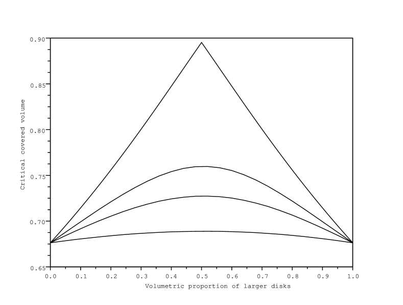
Figure 1: Critical covered volume as a function of $\alpha$ for different values of $\rho$. From bottom to top: $\rho=2,\rho=5,\rho=10$ and the limit as $\rho\to\infty$.

Remarks

• When $\rho\to\infty$, the critical covered volume $\phi(\cdot,\rho)$ converges to $\phi(\cdot,\infty)$ which is symmetric: $\phi(\alpha,\infty)=\phi(1-\alpha,\infty)$. When $\rho$ is finite, the critical covered volume may also look symmetric but Quintanilla and Ziff showed, based on their numerical simulations and statistical analysis, that this was not the case.

• When $\rho$ is finite, the critical covered volume looks concave as a function of $\alpha$. However $\phi(\cdot,\infty)$ is not concave as soon as $\phi_{c}(\delta_{1})<1-\exp(-2)$. Based on (10), $\phi(\cdot,\infty)$ is therefore not concave. As a consequence, at least for large enough $\rho$, $\phi(\cdot,\rho)$ is not concave.

• The numerical results suggests that the minimum of the critical covered fraction is reached when all the disks have the same radius. (Equivalently, for all $\rho$ and all $\alpha$, $\phi(\alpha,\rho)\geq\phi(0,\rho)=\phi(1,\rho)=\phi_{c}(\delta_{1})$.) However there is neither a proof nor a disproof of such a result.

• The numerical results also suggest some monotonicity in $\rho$. This has not been proven nor disproven.

2 Proof of Theorem 4

2.1 Some notations

In the whole of Section 2, we make the following assumptions:

• $\mu$ satisfies (6).

• $1<\widehat{\lambda_{c}}(\mu)$.

For all $\eta>0$, we denote by $T_{\eta}\mu$ the measure defined by $T_{\eta}\mu(A)=\mu(A-\eta)$. In other words, we can built $\Sigma(T_{\eta}\mu)$ from $\Sigma(\mu)$ by adding $\eta$ to each radius.

For all $\rho>1$, we denote by $H^{\rho}\mu$ the measure defined by $H^{\rho}\mu(A)=\rho^{d}\mu(\rho A)$. With this definition, $\rho^{-1}\Sigma(\mu)$ is a Boolean model driven by the measure $H^{\rho}\mu$. For all $n\geq 0$, we let:

$$m_{n}^{\rho}=\sum_{k=0}^{n}H^{\rho^{k}}\mu.$$

With this definition and the notations of (4),

$$\bigcup_{k=0}^{n}\rho^{-k}\Sigma_{k}$$

is a Boolean model driven by $m_{n}^{\rho}$. We also let:

$$m_{\infty}^{\rho}=\sum_{k\geq 0}H^{\rho^{k}}\mu.$$

So, $\Sigma^{\rho}(\mu)$ is a Boolean model driven by the locally finite measure $m_{\infty}^{\rho}$.

Let $p(a,\mu)$ denote the probability of existence of a path from $S(a/2)$ to $S(a)$ in $\Sigma(\mu)$:

$$p(a,\mu)=P(S(a/2)\;\leftrightarrow_{\Sigma(\mu)}\;S(a)).$$

We aim at proving that, for large enough $\rho$, $p(a,m_{\infty}^{\rho})\to 0$ as $a$ tends to infinity and $\Sigma^{\rho}(\mu)$ does not percolate. The first item of Theorem 4 follows by applying this result to the measure $\lambda\mu$. Recall that the second item of Theorem 4 is contained in Theorem 3.

2.2 Ideas

In this subsection we first sketch the proof of the existence of $\rho$ and $a$ such that $p(a,m_{\infty}^{\rho})$ is small. This gives the main ingredients of the proof of the first item of Theorem 4. A full proof is given in Subsection 2.3. We then give the ideas of the proof of Theorems 1 and 2 by Menshikov, Popov and Vachkovskaia. Their basic strategy is similar but the implementation of the proofs are different.

Sketch of the proof of the first item of Theorem 4

Consider a small $\varepsilon_{1}>0$. Fix a small $\eta>0$ and a large $a$ such that (see Lemma 7):

$$p(a,T_{\eta}\mu)\leq\varepsilon_{1}/2.$$ (11)

For all $n\geq 1$, write:

$$m_{n}^{\rho}=H^{\rho}m_{n-1}^{\rho}+\mu.$$

If the event $\{S(a/2)\;\leftrightarrow_{\Sigma(m_{n}^{\rho})}\;S(a)\}$ occurs, then either the event $\{S(a/2)\;\leftrightarrow_{T_{\eta}\mu}\;S(a)\}$ occurs (with a natural coupling between the Boolean models) either in $\Sigma(H^{\rho}m_{n-1}^{\rho})\cap B(a)$ one can find a component of diameter at least $\eta$. We use this observation through its following crude consequence (see Lemma 8):

$$p(a,m_{n}^{\rho})\leq p(a,T_{\eta}\mu)+Ca^{d}\eta^{-d}p(\eta/2,H^{\rho}m_{n-1}^{\rho}).$$

By scaling and by (11), this yields:

$$p(a,m_{n}^{\rho})\leq\varepsilon_{1}/2+Ca^{d}\eta^{-d}p(\rho\eta/2,m_{n-1}^{\rho}).$$ (12)

But for any $\varepsilon_{2}$, any small enough $\varepsilon_{1}$ and any large enough $a$ we can find $\tau$ such that (see Lemmas 9 and 10):

$$p(\tau a,m_{n-1}^{\rho})\leq\varepsilon_{2}\hbox{ as soon as }p(a,m_{n-1}^{\rho})\leq\varepsilon_{1}.$$ (13)

An important fact is that $\tau$ does not depends on $n$ nor on $\rho$, provided $\rho\geq\rho_{0}$ where $\rho_{0}$ is an arbitrary constant strictly larger than $1$. Here we use assumption (6) to bound error terms due to the existence of large balls.

We choose $\varepsilon_{2}$ such that:

$$Ca^{d}\eta^{-d}\varepsilon_{2}=\varepsilon_{1}/2.$$

We set $\rho=2\tau a/\eta$. Then, (12) and (13) can be rewritten as follows:

$$p(a,m_{n}^{\rho}) \leq \varepsilon_{1}/2+Ca^{d}\eta^{-d}p(\tau a,m_{n-1}^{\rho})$$ (14)

$$Ca^{d}\eta^{-d}p(\tau a,m_{n-1}^{\rho}) \leq \varepsilon_{1}/2\hbox{ as soon as }p(a,m_{n-1}^{\rho})\leq\varepsilon_{1}.$$ (15)

As moreover (11) implies $p(a,m_{0}^{\rho})\leq\varepsilon_{1}$ we get, by induction and then sending $n$ to infinity (see Lemma 11):

$$p(a,m_{\infty}^{\rho})\leq\varepsilon_{1}.$$

The convergence of $p(a,m_{\infty}^{\rho})$ to $0$ is then extracted from the above result for a small enough $\varepsilon_{2}$ and from arguments behind (13) applied to $m_{\infty}^{\rho}$ and other $\varepsilon$.

Sketch of the proofs of Theorems 1 and 2 by Menshikov, Popov and Vachkovskaia

Let us quickly describe the ideas of the proofs of Menshikov, Popov and Vachkovskaia. Those ideas are used in their papers [11] and [12] through a discretization of space ; we describe them in a slightly more geometric way. For simplicity we only consider two scales: $\rho^{-1}\Sigma_{1}$ and $\Sigma_{0}$. For simplicity, we also assume that the radius is one in the unscaled model ($\mu=\lambda\delta_{1}$). We assume that the scale factor $\rho$ is large enough. Assume that $C$ is a connected component of $\rho^{-1}\Sigma_{1}\cup\Sigma_{0}$ whose diameter is a least $\alpha$ (it can be much larger) for a small enough constant $\alpha>0$. Then, $C$ is included in the union of the following kind of sets:

1. connected components of $\rho^{-1}\Sigma_{1}$ whose diameter is at least $\alpha$ ;

2. balls of $\Sigma_{0}$ enlarged by $\alpha$ (same centers but the radii are $1+\alpha$ instead of $1$).

Then, they show that the union of all those sets is stochastically dominated by a Boolean model similar to $\Sigma_{0}$ but with radii enlarged by a factor $\alpha$ and with density of centers $1+\alpha^{\prime}$ times the corresponding density for $\Sigma_{0}$ for a suitable $\alpha^{\prime}>0$. This part uses $\lambda<\widehat{\lambda_{c}}$. In some sense, one can therefore control percolation in the union of two models by percolation in one model. Iterating the argument with some care in the constants $\alpha$ and $\alpha^{\prime}$, one sees that – for large enough $\rho$ – one can control percolation in the multiscale model by percolation in a subcritical model. This yields the result.

2.3 Proof of Theorem 4

As $1<\widehat{\lambda_{c}}(\mu)$, we know that $p(a,\mu)$ tends to $0$ as $a$ tends to infinity. We need the following slightly stronger consequence.

Lemma 7

There exists $\eta>0$ such that $p(a,T_{\eta}\mu)$ tends to $0$.

Proof. Let $\varepsilon>0$ and $x>0$. We have:

$$H^{1+\varepsilon}T_{\varepsilon^{2}}\mu([x,+\infty[) = (1+\varepsilon)^{d}T_{\varepsilon^{2}}\mu([x(1+\varepsilon),+\infty[)$$ (16)

$$= (1+\varepsilon)^{d}\mu([x(1+\varepsilon)-\varepsilon^{2},+\infty[)$$

$$\leq \kappa(\varepsilon)(1+\varepsilon)^{d}\mu([x,+\infty[)$$

where

$$\kappa(\varepsilon)=\frac{\mu(]0,+\infty[)}{\mu([\varepsilon,+\infty[)}.$$

The inequality is proven as follows. If $x\geq\varepsilon$, then $[x(1+\varepsilon)-\varepsilon^{2},+\infty[\subset[x,+\infty[$ and the result follows from $\kappa(\varepsilon)\geq 1$. If, on the contrary, $x<\varepsilon$, then the left hand side is bounded above by $(1+\varepsilon)^{d}\mu(]0,+\infty[)$ which is itself bounded above by the right hand side.

Note that $\kappa(\varepsilon)(1+\varepsilon)^{d}$ tends to $1$ as $\varepsilon$ tends to $0$. Let us say that a measure $\nu$ is subcritical if $\widehat{\lambda_{c}}(\nu)>1$. As $\mu$ is subcritical, we get that $\kappa(\varepsilon)(1+\varepsilon)^{d}\mu$ is subcritical for small enough $\varepsilon$. We fix such an $\varepsilon$. By (16) we can couple a Boolean model driven by $H^{1+\varepsilon}T_{\varepsilon^{2}}\mu$ and a Boolean model driven by $\kappa(\varepsilon)(1+\varepsilon)^{d}\mu$ in such a way that the first one is contained in the second one. Therefore the first one is subcritical. By scaling, a Boolean model driven by $T_{\varepsilon^{2}}\mu$ is then subcritical. We take $\eta=\varepsilon^{2}$. $\square$

Lemma 8

Let $\nu_{1}$ and $\nu_{2}$ be two finite measures on $]0,+\infty[$. One has, for all $\eta>0$ and $a\geq 4\eta$:

$$p(a,\nu_{1}+\nu_{2})\leq p(a,T_{\eta}\nu_{1})+C_{1}a^{d}\eta^{-d}p(\eta/2,\nu_{2})$$

where $C_{1}=C_{1}(d)>0$ depends only on the dimension $d$.

Proof. Let $(x_{i})_{i\in I}$ be a family of points such that :

• The balls $B(x_{i},\eta/4)$, $i\leq I$, cover $B(a)$.

• There are at most $C_{1}a^{d}\eta^{-d}$ points in the family where $C_{1}=C_{1}(d)$ depends only on the dimension $d$.

We couple the different Boolean model as follows. Let $\Sigma(\nu_{1})$ be a Boolean model driven by $\nu_{1}$. Let $\Sigma(\nu_{2})$ be a Boolean model driven by $\nu_{2}$. Assume that $\Sigma(\nu_{1})$ and $\Sigma(\nu_{2})$ are independent. Then $\Sigma(\nu_{1})\cup\Sigma(\nu_{2})$ is a Boolean model driven by $\nu_{1}+\nu_{2}$. We set $\Sigma(\nu_{1}+\nu_{2})=\Sigma(\nu_{1})\cup\Sigma(\nu_{2})$. We also consider $\Sigma(T_{\eta}\nu_{1})$, the Boolean model obtained by adding $\eta$ to the radius of each ball of $\Sigma(\nu_{1})$. Thus $\Sigma(T_{\eta}\nu_{1})$ is driven by $T_{\eta}\nu_{1}$.

Let us prove the following property:

$$\{S(a/2)\;\leftrightarrow_{\Sigma(\nu_{1}+\nu_{2})}\;S(a)\}\subset\{S(a/2)\;\leftrightarrow_{\Sigma(T_{\eta}\nu_{1})}\;S(a)\}\cup\bigcup_{i\in I}\{S(x_{i},\eta/4)\;\leftrightarrow_{\Sigma(\nu_{2})}\;S(x_{i},\eta/2)\}.$$ (17)

Assume that $\Sigma(\nu_{1}+\nu_{2})=\Sigma(\nu_{1})\cup\Sigma(\nu_{2})$ connects $S(a/2)$ with $S(a)$. Recall $a\geq 4\eta$. If the diameter of all connected components of $\Sigma(\nu_{2})\cap B(a)$ are less or equal to $\eta$, then $\Sigma(T_{\eta}\nu_{1})$ connects $S(a/2)$ with $S(a)$. Otherwise, let $C$ be a connected component of $\Sigma(\nu_{2})\cap B(a)$ with diameter at least $\eta$. Let $x,y$ be two points of $C$ such that $\|x-y\|>\eta$. The point $x$ belongs to a ball $B(x_{i},\eta/4)$. As $y$ does not belong to $B(x_{i},\eta/2)$, the component $C$ connects $S(x_{i},\eta/4)$ to $S(x_{i},\eta/2)$. Therefore, $\Sigma(\nu_{2})$ connects $S(x_{i},\eta/4)$ to $S(x_{i},\eta/2)$. We have proven (17). The lemma follows. $\square$

The following lemma is essentially the first item of Proposition 3.1 in [4]. For the sake of completeness we nevertheless provide a proof.

Lemma 9

Let $\nu$ be a finite measure on $]0,+\infty[$. There exists a constant $C_{2}=C_{2}(d)>0$ such that, for all $a>0$:

$$p(10a,\nu)\leq C_{2}p(a,\nu)^{2}+C_{2}\int_{[a,+\infty[}r^{d}\nu(dr).$$

Proof. Let $K$ be a finite subset of $S(5)$ such that $K+B(1/2)$ covers $S(5)$. Let $L$ be a finite subset of $S(10)$ such that $L+B(1/2)$ covers $S(10)$. Let $A$ be the following event: there exists a random ball $B(c,r)$ of $\Sigma(\nu)$ such that $r\geq a$ and $B(c,r)\cap B(10a)$ is non empty. We have:

$$\{S(5a)\;\leftrightarrow_{\Sigma(\nu)}\;S(10a)\}\setminus A\subset\{S(5a)\;\leftrightarrow_{\Sigma(\nu)}^{\leq a}\;S(10a)\}$$

where, in the last event, we ask for a path using only balls of $\Sigma(\nu)$ of radius at most $a$. Let us prove the following:

$$\{S(5a)\;\leftrightarrow_{\Sigma(\nu)}\;S(10a)\}\setminus A\\ \subset\bigcup_{k\in K,l\in L}\{S(ak,a/2)\;\leftrightarrow_{\Sigma(\nu)}^{\leq a}\;S(ak,a)\}\cap\{S(al,a/2)\;\leftrightarrow_{\Sigma(\nu)}^{\leq a}\;S(al,a)\}.$$ (18)

Assume that the event on the left hand side occurs. Then, by the previous remark, there exists a path from a point $x\in S(5a)$ to a point $y\in S(10a)$ that is contained in balls of $\Sigma(\nu)$ of radius at most $a$. As $Ka+B(a/2)$ covers $S(5a)$, there exists $k\in K$ such that $x$ belongs to $B(ka,a/2)$. Using the previous path, one gets that the event

$$\{S(ak,a/2)\;\leftrightarrow_{\Sigma(\nu)}^{\leq a}\;S(ak,a)\}$$

occurs. By a similar arguments involving $y$ we get (18).

Observe that, for all $k\in K$ and $l\in L$, the events

$$\{S(ak,a/2)\;\leftrightarrow_{\Sigma(\nu)}^{\leq a}\;S(ak,a)\}\hbox{ and }\{S(al,a/2)\;\leftrightarrow_{\Sigma(\nu)}^{\leq a}\;S(al,a)\}$$

are independent. Indeed, the first one depends only on balls with centers in $B(ak,2a)$, the second one depends only on balls with centers in $B(al,2a)$, and $\|ak-al\|\geq 5a$. Using this independence, stationarity and (18), we then get:

$$P(\{S(5a)\;\leftrightarrow_{\Sigma(\nu)}\;S(10a)\})\leq CP(S(a/2)\;\leftrightarrow_{\Sigma(\nu)}^{\leq a}\;S(a)\})^{2}+P(A)$$

where $C$ is the product of the cardinality of $K$ by the cardinality of $L$. The probability $P(A)$ is bounded above by standard computations. $\square$

From the previous lemma, we deduce the following result.

Lemma 10

Let $\varepsilon>0$. There exists $C_{3}=C_{3}(d)>0$, $a_{0}=a_{0}(d,\mu)$ and $k_{0}=k_{0}(d,\mu,\varepsilon)$ such that, for all $N$, all $\rho\geq 2$ and all $a\geq a_{0}$: if $p(a,m^{\rho}_{N})\leq C_{3}$ then for all $k\geq k_{0}$, $p(a10^{k},m^{\rho}_{N})\leq\varepsilon$.

Proof. For all $\rho\geq 2$ and all $a\geq 1$ we have:

$$\int_{[a,+\infty[}r^{d}m^{\rho}_{\infty}(dr) = \sum_{k\geq 0}\rho^{kd}\int_{]0,+\infty[}1_{[a,+\infty[}(r\rho^{-k})(r\rho^{-k})^{d}\mu(dr)$$

$$= \int_{]0,+\infty[}\sum_{k\geq 0}1_{[a,+\infty[}(r\rho^{-k})r^{d}\mu(dr)$$

$$= \int_{[a,+\infty[}\big{(}\left\lfloor\ln(r/a)\ln(\rho)^{-1}\right\rfloor+1\big{)}r^{d}\mu(dr)$$

$$\leq \int_{[a,+\infty[}(\ln(r)\ln(2)^{-1}+1)r^{d}\mu(dr).$$

Let $C_{2}$ be the constant given by Lemma 9. By (6) we can chose $a_{0}=a_{0}(d,\mu)\geq 1$ such that

$$C_{2}^{2}\int_{[a_{0},+\infty[}(\ln(r)\ln(2)^{-1}+1)r^{d}\mu(dr)\leq\frac{1}{4}.$$ (19)

Let $C_{3}=(2C_{2})^{-1}$. Let $N$, $\rho$ and $a$ be as in the statement of the lemma. From Lemma 9 we get:

$$C_{2}p(10a,m^{\rho}_{N}) \leq (C_{2}p(a,m^{\rho}_{N}))^{2}+C_{2}^{2}\int_{[a,+\infty[}r^{d}m^{\rho}_{N}(dr)$$ (20)

$$\leq (C_{2}p(a,m^{\rho}_{N}))^{2}+C_{2}^{2}\int_{[a,+\infty[}(\ln(r)\ln(2)^{-1}+1)r^{d}\mu(dr)$$ (21)

Let $(u_{k})$ be a sequence defined by $u_{0}=1/2$ and, for all $k\geq 0$:

$$u_{k+1}=u_{k}^{2}+C_{2}^{2}\int_{[a_{0}10^{k},+\infty[}(\ln(r)\ln(2)^{-1}+1)r^{d}\mu(dr).$$ (22)

Note that the sequence $(u_{k})$ only depends on $d$ and $\mu$.

Assume that $p(a,m^{\rho}_{N})\leq C_{3}$. We then have $C_{2}p(a,m^{\rho}_{N})\leq u_{0}$. Using $a\geq a_{0}$ and (21), we then get $C_{2}p(a10^{k},m^{\rho}_{N})\leq u_{k}$ for all $k$. Therefore, it sufficies to show that the sequence $(u_{k})$ tends to $0$.

Using (22), (19) and $u_{0}=1/2$ we get $0\leq u_{k}\leq 1/2$ for all $k$. Therefore, $0\leq\limsup u_{k}\leq 1/2$. By (22) and by the convergence of the integrale we also get $\limsup u_{k}\leq(\limsup u_{k})^{2}$. As a consequence, $\limsup u_{k}=0$ and the lemma is proven. $\square$

Lemma 11

For all $a>0$ and $\rho>1$ the following convergence holds:

$$p(a,m^{\rho}_{\infty})=\lim_{N\to\infty}p(a,m^{\rho}_{N}).$$

Proof. The sequence of events

$$A_{N}=\{S(a/2)\;\leftrightarrow_{\Sigma(m^{\rho}_{N})}\;S(a)\}$$

is increasing (we use the natural coupling between our Boolean models). Therefore, it suffices to show that the union of the previous events is

$$A=\{S(a/2)\;\leftrightarrow_{\Sigma(m^{\rho}_{\infty})}\;S(a)\}.$$

If $A$ occurs, then there is is path from $S(a/2)$ to $S(a)$ that is contained in $\Sigma(m^{\rho}_{\infty})$. By a compactness argument, this path is included in a finite union of ball of $\Sigma(m^{\rho}_{\infty})$. Therefore, there exists $N$ such that the path is included in $\Sigma(m^{\rho}_{N})$ and $A_{N}$ occurs. This proves $A\subset\cup A_{N}$. The other inclusion is straightforward. $\square$

Proof of the second item of Theorem 4. By Lemma 7, we can fix $\eta_{1}>0$ such that $p(a,T_{10\eta_{1}}\mu)$ tends to $0$ as $a$ tends to $\infty$. Let $C_{1}$ be given by Lemma 8. Let $a_{0}$ and $C_{3}$ be as given by Lemma 10. Fix $a_{1}\geq\max(40\eta_{1},a_{0},1)$ such that $p(a,T_{10\eta_{1}}\mu)\leq C_{3}/2$ for all $a\geq a_{1}$. Let $k_{0}$ be given by Lemma 10 with the choice:

$$\varepsilon=C_{1}^{-1}(10a_{1})^{-d}\eta_{1}^{d}C_{3}/2.$$

Therefore, for all $\rho\geq 2$, all $N$, all $a\in[a_{1},10a_{1}]$ and all $\eta\in[\eta_{1},10\eta_{1}]$:

$$C_{1}a^{d}\eta^{-d}p(a10^{k},m_{N}^{\rho})\leq\frac{C_{3}}{2}\hbox{ for all }k\geq k_{0}\hbox{ as soon as }p(a,m_{N}^{\rho})\leq C_{3}.$$

Fix $k\geq k_{0}$, $a\in[a_{1},10a_{1}]$ and $\eta\in[\eta_{1},10\eta_{1}]$. Set:

$$\rho=2a10^{k}\eta^{-1}.$$

Note $\rho\geq 8\geq 2$ as $a\geq a_{1}\geq 40\eta_{1}\geq 4\eta$. By Lemma 8 we have, for all $N$:

$$p(a,m_{N+1}^{\rho}) \leq p(a,T_{\eta}\mu)+C_{1}a^{d}\eta^{-d}p(\eta/2,m^{\rho}_{N+1}-\mu)$$

$$= p(a,T_{\eta}\mu)+C_{1}a^{d}\eta^{-d}p(\eta/2,H^{\rho}m_{N}^{\rho}).$$

By definition of $a_{1}$, by $a_{1}\leq a$, by $\eta\leq 10\eta_{1}$, by scaling and by definition of $\rho$ we get, for all $N$:

$$p(a,m_{N+1}^{\rho}) \leq \frac{C_{3}}{2}+C_{1}a^{d}\eta^{-d}p(\rho\eta/2,m_{N}^{\rho})$$

$$= \frac{C_{3}}{2}+C_{1}a^{d}\eta^{-d}p(a10^{k},m_{N}^{\rho}).$$

Combining this inequality with the property defining $k_{0}$, we get that $p(a,m_{N}^{\rho})\leq C_{3}$ implies $p(a,m_{N+1}^{\rho})\leq C_{3}$. As $p(a,m_{0}^{\rho})=p(a,\mu)\leq p(a,T_{10\eta_{1}}\mu)\leq C_{3}/2$ we get $p(a,m_{N}^{\rho})\leq C_{3}$ for all integer $N$.

Let $\varepsilon>0$. Using again Lemma 10 we get the existence of an integer $k^{\prime}_{0}$ such that $p(a10^{k^{\prime}},m_{N}^{\rho})\leq\varepsilon$ for all $k^{\prime}\geq k^{\prime}_{0}$ as soon as $p(a,m_{N}^{\rho})\leq C_{3}$. But we have proven the latter property. Therefore $p(a10^{k^{\prime}},m_{N}^{\rho})\leq\varepsilon$ for all $N$ and all $k^{\prime}\geq k^{\prime}_{0}$. By Lemma 11, we get $p(a10^{k^{\prime}},m_{\infty}^{\rho})\leq\varepsilon$ for all $k^{\prime}\geq k^{\prime}_{0}$. Using the freedom on the choice of $k\geq k_{0}$ and $\eta\in[\eta_{1},10\eta_{1}]$, we get that the previous result holds for all $\rho\geq 2a10^{k_{0}-1}\eta_{1}^{-1}$ and then for all $\rho\geq 2a_{1}10^{k_{0}}\eta_{1}^{-1}$. Moreover, using the freedom on the choice of $a\in[a_{1},10a_{1}]$ and $k^{\prime}\geq k^{\prime}_{0}$, we get:

$$p(r,m_{\infty}^{\rho})\leq\varepsilon\hbox{ for all }r\geq a_{1}10^{k^{\prime}_{0}}\hbox{ and all }\rho\geq 2a_{1}10^{k_{0}}\eta_{1}^{-1}.$$

Therefore, $p(r,m_{\infty}^{\rho})$ tends to $0$ as $r$ tends to infinity. As a consequence, $\Sigma^{\rho}(\mu)$ does not percolate for any $\rho\geq 2a_{1}10^{k_{0}}\eta_{1}^{-1}$. $\square$

3 Proof of Theorem 5

Lemma 12

Let $s>0$ and $\rho>1$. The following assumptions are equivalent:

1. $\int_{]0,+\infty[}r^{d+s}\mu(dr)<\infty$.

2. $\int_{[1,+\infty[}r^{d+s}m_{\infty}^{\rho}(dr)<\infty$.

Proof. We have:

$$\int_{[1,+\infty[}r^{d+s}m^{\rho}_{\infty}(dr) = \sum_{k\geq 0}\rho^{kd}\int_{]0,+\infty[}1_{[1,+\infty[}(r\rho^{-k})(r\rho^{-k})^{d+s}\mu(dr)$$

$$= \int_{[1,+\infty[}\sum_{k\geq 0}1_{[1,+\infty[}(r\rho^{-k})\rho^{-ks}r^{d+s}\mu(dr).$$

Therefore:

$$\int_{[1,+\infty[}r^{d+s}\mu(dr)\leq\int_{[1,+\infty[}r^{d+s}m^{\rho}_{\infty}(dr)\leq\frac{1}{1-\rho^{-s}}\int_{[1,+\infty[}r^{d+s}\mu(dr).$$

This yields the result. $\square$

Proof of the first item of Theorem 5. By the discussion at the beginning of Section 1.5 in [5], $\Sigma^{\rho}(\lambda\mu)$ is driven by a a Poisson point process whose intensity is the product of the Lebesgue measure by the locally finite measure $\lambda m_{\infty}^{\rho}$. Let us check the three items of Theorem 2.9 in [5] with $\rho=10$ ($\rho$ is not use in the same way in [5]). We refer to Section 2.1 of [5] for definitions.

1. The first item is fulfilled thanks to (7)

2. For all $\beta>0$ and all $x\in\mathbb{R}^{d}$, the event $G(x,0,\beta)$ only depends on balls $B(c,r)\in\Sigma^{\rho}(\lambda\mu)$ such that $c$ belongs to $B(x,3\beta)$. By the independance property of Poisson point processes, we then get that $G(0,0,\beta)$ and $G(x,0,\beta)$ are independent whenever $\|x\|\geq 10\beta$. Therefore $I(10,0,\beta)=0$ and the second item of Theorem 2.9 is fulfilled.

3. The third item (note that $\mu$ in [5] is $m_{\infty}^{\rho}$ in this paper) is fulfilled thanks to Lemma 12

Theorem 2.9 in [5] yields the result. $\square$

Proof of the second item of Theorem 5. If $\int r^{d}\mu(dr)$ is infinite then, $\Sigma(\lambda\mu)$ percolates for all $\lambda>0$ (see the dicussion of Section 1.2). Therefore $\Sigma^{\rho}(\lambda\mu)$ percolates for all $\rho>1$ and $\lambda>0$. Therefore $D^{\rho}(\lambda\mu)=\infty$ with positive probability for all $\rho>1$ and $\lambda>0$.

Now, assume that $\int r^{d}\mu(dr)$ is finite. Then, by the discussion at the beginning of Section 1.5 in [5], $\Sigma^{\rho}(\lambda\mu)$ is driven by a a Poisson point process whose intensity is the product of the Lebesgue measure by the locally finite measure $\lambda m_{\infty}^{\rho}$. We can therefore apply Theorem 1.2 in [5]. By Lemma 12, assumption (A3) of Theorem 1.2 in [5] is not fulfilled (note that $\mu$ in [5] is $m_{\infty}^{\rho}$ in this paper). Theorem 1.2 in [5] then yields the result. $\square$

4 Proof of Proposition 6

We first need a lemma, which is a consequence of Lemmas 8 and 9.

Lemma 13

Let $\nu_{1}$ and $\nu_{2}$ be two finite measures on $]0,+\infty[$. Let $\eta>0$ and $a_{0}\geq 4\eta$. Let $\rho>1$. There exists $C_{4}=C_{4}(d)>0$ such that $\widehat{\lambda}_{c}(\nu_{1}+H_{\rho}(\nu_{2}))\geq 1$ as soon as the following conditions hold:

1. $p(a,T_{\eta}\nu_{1})\leq C_{4}$ for all $a\in[a_{0},10a_{0}]$.

2. $a_{0}^{d}\eta^{-d}p(\rho\eta/2,\nu_{2})\leq C_{4}$.

3. $\int_{[a_{0},+\infty[}r^{d}\nu_{1}(dr)\leq C_{4}$ and $\int_{[a_{0},+\infty[}r^{d}\nu_{2}(dr)\leq C_{4}$.

Proof. Let $C_{4}=C_{4}(d)>0$ be such that $C_{4}C_{2}(1+10^{d}C_{1})\leq 1/2$ and $2C_{2}^{2}C_{4}\leq 1/4$, where $C_{1}$ appears in Lemma 8 and $C_{2}$ appears in Lemma 9. Set $\nu=\nu_{1}+H_{\rho}(\nu_{2})$.

For all $a\in[a_{0},10a_{0}]$ we have, by Lemma 8 applied to $\nu_{1}$ and $H_{\rho}(\nu_{2})$, by scaling and by the assumptions of the lemma:

$$p(a,\nu) \leq p(a,T_{\eta}\nu_{1})+C_{1}a^{d}\eta^{-d}p(\eta/2,H_{\rho}\nu_{2})$$ (23)

$$= p(a,T_{\eta}\nu_{1})+C_{1}a^{d}\eta^{-d}p(\rho\eta/2,\nu_{2})$$

$$\leq C_{4}(1+10^{d}C_{1})$$

$$\leq 1/(2C_{2}).$$

But for all $a\geq a_{0}$ we have, by Lemma 9 and by the assumptions of the lemma:

$$C_{2}p(10a,\nu) \leq (C_{2}p(a,\nu))^{2}+C_{2}^{2}\int_{[a,+\infty[}r^{d}\nu(dr)$$

$$= (C_{2}p(a,\nu))^{2}+C_{2}^{2}\int_{[a,+\infty[}r^{d}\nu_{1}(dr)+C_{2}^{2}\int_{[a\rho,+\infty[}r^{d}\nu_{2}(dr)$$

$$\leq (C_{2}p(a,\nu))^{2}+2C_{2}^{2}C_{4}$$

$$\leq (C_{2}p(a,\nu))^{2}+1/4.$$ (25)

By (23) and (25) we get $C_{2}p(a,\nu)\leq 1/2$ for all $a\geq a_{0}$ and therefore $0\leq\limsup C_{2}p(a,\nu)\leq 1/2$. By (4) and the third assumption of the lemma, we get $\limsup C_{2}p(a,\nu)\leq(\limsup C_{2}p(a,\nu))^{2}$. Therefore, we must have $\limsup C_{2}p(a,\nu)=0$ and the lemma is proven. $\square$

Proof of Proposition 6. The inequality is straightforward. To prove the inequality, we note that, by scaling, $\widehat{\lambda}_{c}(H_{\rho}\nu_{2})=\widehat{\lambda}_{c}(\nu_{2})$. Let us prove the convergence. We can assume $\widehat{\lambda}_{c}(\nu_{1})>0$ and $\widehat{\lambda}_{c}(\nu_{2})>0$, otherwise the convergence is obvious. Therefore, by Lemma 15, the integrals $\int r^{d}\nu_{1}(dr)$ and $\int r^{d}\nu_{2}(dr)$ are finite.

Let $C_{4}$ be the constant given by Lemma 13. Let $0<\varepsilon<1$. Note:

$$\widehat{\lambda_{c}}\big{(}(1-\varepsilon)\widehat{\lambda}_{c}(\nu_{1})\nu_{1}\big{)}=(1-\varepsilon)^{-1}\widehat{\lambda}_{c}(\nu_{1})^{-1}\widehat{\lambda}_{c}(\nu_{1})>1,$$

Therefore, by Lemma 7 (in which (6) is not used), we can fix $\eta>0$ such that

$$p(a,T_{\eta}(1-\varepsilon)\widehat{\lambda}_{c}(\nu_{1})\nu_{1})\to 0.$$

We can then fix $a_{0}\geq 4\eta$ such that:

$$p(a,T_{\eta}(1-\varepsilon)\widehat{\lambda}_{c}(\nu_{1})\nu_{1})\leq C_{4}\hbox{ for all }a\geq a_{0}$$ (26)

and such that

$$\int_{[a_{0},+\infty[}r^{d}\widehat{\lambda}_{c}(\nu_{1})\nu_{1}(dr)\leq C_{4}$$ (27)

and

$$\int_{[a_{0},+\infty[}r^{d}\widehat{\lambda}_{c}(\nu_{2})\nu_{2}(dr)\leq C_{4}.$$ (28)

Now we fix $\rho_{0}>1$ such that :

$$a_{0}^{d}\eta^{-d}p(\rho\eta/2,(1-\varepsilon)\widehat{\lambda}_{c}(\nu_{2})\nu_{2})\leq C_{4}\hbox{ for all }\rho\geq\rho_{0}.$$ (29)

Now, let $0<\alpha<1$ and let

$$\lambda=\min\left(\frac{\widehat{\lambda}_{c}(\nu_{1})(1-\varepsilon)}{\alpha},\frac{\widehat{\lambda}_{c}(\nu_{2})(1-\varepsilon)}{1-\alpha}\right).$$

By (26), (29), (27) and (28) we get that Assumptions 1 , 2 and 3 of Lemma 13 are fulfilled for the measures $\alpha\lambda\nu_{1}$ and $(1-\alpha)\lambda\nu_{2}$ and for $\rho\geq\rho_{0}$. Therefore, we get

$$\widehat{\lambda}_{c}(\alpha\lambda\nu_{1}+(1-\alpha)\lambda H_{\rho}\nu_{2})\geq 1$$

and thus:

$$\widehat{\lambda}_{c}(\alpha\nu_{1}+(1-\alpha)H_{\rho}\nu_{2})\geq\lambda=(1-\varepsilon)\min\left(\frac{\widehat{\lambda}_{c}(\nu_{1})}{\alpha},\frac{\widehat{\lambda}_{c}(\nu_{2})}{1-\alpha}\right).$$

Therefore, as soon as $\rho\geq\rho_{0}$, we have:

$$0 \leq \min\left(\frac{\widehat{\lambda}_{c}(\nu_{1})}{\alpha},\frac{\widehat{\lambda}_{c}(\nu_{2})}{1-\alpha}\right)-\widehat{\lambda}_{c}(\alpha\nu_{1}+(1-\alpha)H_{\rho}\nu_{2})$$

$$\leq \varepsilon\min\left(\frac{\widehat{\lambda}_{c}(\nu_{1})}{\alpha},\frac{\widehat{\lambda}_{c}(\nu_{2})}{1-\alpha}\right)$$

$$\leq \varepsilon\max(2\widehat{\lambda}_{c}(\nu_{1}),2\widehat{\lambda}_{c}(\nu_{2})).$$

This yields the proposition. $\square$

Appendix A Critical parameters

Lemma 14

$$\widetilde{\lambda_{c}}(\mu)\leq\widehat{\lambda_{c}}(\mu)\leq\lambda_{c}(\mu).$$

Proof. The second inequality is a consequence of the following inclusion:

$$\{\{0\}\;\leftrightarrow_{\Sigma}\;S(r)\}\subset\{S(r/2)\;\leftrightarrow_{\Sigma}\;S(r)\}.$$

The first inequality can be proven as follows. Let $r\geq 1$. By the FKG inequality, we get:

$$P(\{0\}\;\leftrightarrow_{\Sigma}\;S(r)) \geq P(B(0,1)\subset\Sigma\hbox{ and }S(1)\;\leftrightarrow_{\Sigma}\;S(r))$$

$$\geq CP(S(1)\;\leftrightarrow_{\Sigma}\;S(r))$$

where $C=P(B(0,1)\subset\Sigma)>0$ does not depend on $r$. For all large enough $r$, we can cover $S(2r)$ by at most $C^{\prime}r^{d}$ balls $B(x_{i},1)$ where $C^{\prime}$ only depends on the dimension $d$. If there is a path in $\Sigma$ from $S(2r)$ to $S(4r)$, then there exists $i$ and a path in $\Sigma$ from $S(x_{i},1)$ to $S(x_{i},r)$. (Consider the ball $B(x_{i},1)$ that contains the initial point of the path.) By stationarity and by the previous inequality we thus get:

$$P(S(2r)\;\leftrightarrow_{\Sigma}\;S(4r)) \leq C^{\prime}r^{d}P(S(1)\;\leftrightarrow_{\Sigma}\;S(r))$$

$$\leq C^{\prime}C^{-1}r^{d}P(\{0\}\;\leftrightarrow_{\Sigma}\;S(r)).$$

The first inequality stated in the lemma follows. $\square$

Lemma 15

The treshold parameter $\widehat{\lambda_{c}}(\mu)$ is positive if and only if $\int r^{d}\mu(dr)$ is finite.

Proof. If $\widehat{\lambda_{c}}(\mu)$ is positive, then there exists $\lambda>0$ such that $\Sigma(\lambda\mu)$ does not percolate. By Theorem 2.1 of [4] this implies that $\int r^{d}\mu(dr)$ is finite.

Let us assume now that $\int r^{d}\mu(dr)$ is finite. We need to prove the existence of $\lambda>0$ such that $p(a,\lambda\mu)$ tends to $0$. This is proven, as an intermediate result, in the proof of Theorem 1.1 in [5]. As the result is an easy consequence of Lemma 9, we find it more convenient to provide a proof here. Let $C_{2}$ be the constant given by Lemma 9. For all $a>0$ and $\lambda>0$ we have:

$$C_{2}p(10a,\lambda\mu)\leq(C_{2}p(a,\lambda\mu))^{2}+\lambda C_{2}^{2}\int_{[a,+\infty[}r^{d}\mu(dr).$$ (30)

For all $0<a\leq 1$ we have, by standard computations:

$$C_{2}p(a,\lambda\mu)\leq C_{2}P(\hbox{a ball of }\Sigma(\lambda\mu)\hbox{ touches }B(a))\leq C_{2}v_{d}\lambda\int_{]0,+\infty[}(1+r)^{d}\mu(dr)$$

where $v_{d}$ is the volume of the unit Euclidean ball. As $\int r^{d}\mu(dr)$ is finite, we can therefore fix $\lambda>0$ such that:

$$\lambda C_{2}^{2}\int_{[a,+\infty[}r^{d}\mu(dr)\leq 1/4\hbox{ for all }a>0\hbox{ and }C_{2}p(a,\lambda\mu)\leq 1/2\hbox{ for all }0<a\leq 1.$$ (31)

By (30), (31) and by induction we get $C_{2}p(a,\lambda\mu)\leq 1/2$ for all $a>0$. Therefore, we have $0\leq\limsup C_{2}p(a,\lambda\mu)\leq 1/2$. But (30) also yields the inequality $\limsup C_{2}p(a,\lambda\mu)\leq(\limsup C_{2}p(a,\lambda\mu))^{2}$. As a consequence we must have $\limsup C_{2}p(a,\lambda\mu)=0$ and then $p(a,\lambda\mu)\to 0$. $\square$

References

- [1] Erik I. Broman and Federico Camia. Large- limit of crossing probabilities, discontinuity, and asymptotic behavior of threshold values in Mandelbrot’s fractal percolation process. Electron. J. Probab., 13:no. 33, 980–999, 2008.
- [2] Erik I. Broman and Federico Camia. Universal behavior of connectivity properties in fractal percolation models. 2009.
- [3] Lincoln Chayes. Aspects of the fractal percolation process. In Fractal geometry and stochastics (Finsterbergen, 1994), volume 37 of Progr. Probab., pages 113–143. Birkhäuser, Basel, 1995.
- [4] Jean-Baptiste Gouéré. Subcritical regimes in the Poisson Boolean model of continuum percolation. Ann. Probab., 36(4):1209–1220, 2008.
- [5] Jean-Baptiste Gouéré. Subcritical regimes in some models of continuum percolation. Ann. Appl. Probab., 19(4):1292–1318, 2009.
- [6] Geoffrey Grimmett. Percolation, volume 321 of Grundlehren der Mathematischen Wissenschaften [Fundamental Principles of Mathematical Sciences]. Springer-Verlag, Berlin, second edition, 1999.
- [7] Peter Hall. On continuum percolation. Ann. Probab., 13(4):1250–1266, 1985.
- [8] M. Mandelbrot. Intermittent turbulence in self-similar cascades: divergence of high moments and dimension of the carrier. Journal of Fluid Mechanics, 62:331–358, 1974.
- [9] Ronald Meester and Rahul Roy. Continuum percolation, volume 119 of Cambridge Tracts in Mathematics. Cambridge University Press, Cambridge, 1996.
- [10] Ronald Meester, Rahul Roy, and Anish Sarkar. Nonuniversality and continuity of the critical covered volume fraction in continuum percolation. J. Statist. Phys., 75(1-2):123–134, 1994.
- [11] M. V. Menshikov, S. Yu. Popov, and M. Vachkovskaia. On the connectivity properties of the complementary set in fractal percolation models. Probab. Theory Related Fields, 119(2):176–186, 2001.
- [12] M. V. Menshikov, S. Yu. Popov, and M. Vachkovskaia. On a multiscale continuous percolation model with unbounded defects. Bull. Braz. Math. Soc. (N.S.), 34(3):417–435, 2003. Sixth Brazilian School in Probability (Ubatuba, 2002).
- [13] M. V. Men′shikov and A. F. Sidorenko. Coincidence of critical points in Poisson percolation models. Teor. Veroyatnost. i Primenen., 32(3):603–606, 1987.
- [14] S. A. Molchanov, V. F. Pisarenko, and A. Ya. Reznikova. Multiscale models of failure and percolation. Physics of The Earth and Planetary Interiors, 61(1-2):36–43, 1990.
- [15] M. E. Orzechowski. On the phase transition to sheet percolation in random Cantor sets. J. Statist. Phys., 82(3-4):1081–1098, 1996.
- [16] Serguei Yu. Popov and Marina Vachkovskaia. A note on percolation of Poisson sticks. Braz. J. Probab. Stat., 16(1):59–67, 2002.
- [17] John A. Quintanilla and Robert M. Ziff. Asymmetry in the percolation thresholds of fully penetrable disks with two different radii. Phys. Rev. E, 76(5):051115, Nov 2007.
- [18] Damien G. White. On the value of the critical point in fractal percolation. Random Structures Algorithms, 18(4):332–345, 2001.
- [19] S. A. Zuev and A. F. Sidorenko. Continuous models of percolation theory. I. Teoret. Mat. Fiz., 62(1):76–86, 1985.
- [20] S. A. Zuev and A. F. Sidorenko. Continuous models of percolation theory. II. Teoret. Mat. Fiz., 62(2):253–262, 1985.