Lévy Fluctuations and Tracer Diffusion in Dilute Suspensions of Algae and Bacteria

Abstract

Swimming microorganisms rely on effective mixing strategies to achieve efficient nutrient influx. Recent experiments, probing the mixing capability of unicellular biflagellates, revealed that passive tracer particles exhibit anomalous non-Gaussian diffusion when immersed in a dilute suspension of self-motile Chlamydomonas reinhardtii algae. Qualitatively, this observation can be explained by the fact that the algae induce a fluid flow that may occasionally accelerate the colloidal tracers to relatively large velocities. A satisfactory quantitative theory of enhanced mixing in dilute active suspensions, however, is lacking at present. In particular, it is unclear how non-Gaussian signatures in the tracers’ position distribution are linked to the self-propulsion mechanism of a microorganism. Here, we develop a systematic theoretical description of anomalous tracer diffusion in active suspensions, based on a simplified tracer-swimmer interaction model that captures the typical distance scaling of a microswimmer’s flow field. We show that the experimentally observed non-Gaussian tails are generic and arise due to a combination of truncated Lévy statistics for the velocity field and algebraically decaying time correlations in the fluid. Our analytical considerations are illustrated through extensive simulations, implemented on graphics processing units to achieve the large sample sizes required for analyzing the tails of the tracer distributions.

Brownian motion presents one of the most beautiful manifestations of the central limit theorem in Nature 2005HaMa_R . Reported as early as 1784 by the Dutch scientist Jan van Ingenhousz 1784IH , the seemingly unspectacular random motion of mesoscopic particles in a liquid environment made an unforeseeable impact when Perrin’s seminal experiments of 1909 1909Pe yielded convincing evidence for the atomistic structure of liquids. This major progress in our understanding of non-living matter – which happened long before direct observations of atoms and molecules came within experimental reach – would not have been possible without the works of Sutherland 1905Su and Einstein 1905Einstein_BM , who were able to link the microscopic properties of liquids to a macroscopic observable, namely the mean square displacement of a colloidal test particle.

Caused by many quasi-independent random collisions with surrounding molecules, Brownian motion in a passive liquid is quintessentially Gaussian, as predicted by the central limit theorem. Remarkably, however, recent experiments by Leptos et al. 2009LeEtAl_Gold revealed notable non-Gaussian features in the probability distribution of a tracer particle, when a small concentration of microscale swimmers, in their case unicellular biflagellate Chlamydomonas reinhardtii algae, was added to the fluid. Understanding this apparent violation of the central limit theorem presents a challenging unsolved problem, whose solution promises new insights into the mixing strategies of microorganisms 1977Pu . Here, we shall combine extensive analytic and large-scale numerical calculations to elucidate the intimate connection between the flow field of an individual microorganism and the anomalous (non-Gaussian) diffusion of tracer particles in a dilute swimmer suspension.

Modern high-speed microscopy techniques resolve the stochastic dynamics of micron-sized tracer particles to an ever increasing accuracy 2006Lubensky ; 2010Li . This opens the exciting possibility of using high-precision tracking experiments to probe the statistics of the flow fields created by active swimmers, and hence their connection to physical properties and evolutionary strategies of microorganisms that live in liquid environments 2009PoEtAl_Gold ; 2010Drescher_PNAS ; 2009LeEtAl_Gold . Furthermore, a novel class of micromechanical devices 2009So ; 2010Le use nonequilibrium fluctuations generated by bacteria as a fundamental ingredient of their operation. To explain and exploit the nonequilibrium conditions in active suspensions, it is important to fully understand the relation between the experimentally observed features of tracer displacements and the characteristics (such as self-propulsion mechanisms) of the algae or bacteria.

The observations of Leptos et al. 2009LeEtAl_Gold demonstrate that the time-dependent probability distributions of tracer displacements in dilute algae suspensions exhibit tails that decay much more slowly than would be expected if the tracers obeyed purely Gaussian statistics. At high swimmer concentrations, enhanced transport might be expected 2000WuLi_PRL ; 2007LuYo_PRL ; 2005HeOr_PRL ; 2008UnHe_PRL , as collective behavior emerges from swimmer interactions, which can lead to the formation of large-scale vortices and jets. In dilute suspensions, however, where swimmer-swimmer interactions can be neglected, a satisfactory quantitative understanding of the underlying velocity statistics is still lacking. Below, we are going to show that the velocity distribution produced by the swimmers takes a tempered (or regularized) Lévy form 2000MeKl ; 2004MeKl , and that the long-time behavior of the tracers’ positional probability distribution function can be understood in terms of correlated truncated Lévy flights 1994Stanley .

If a microswimmer is self-propelled, with no external forces acting, its flow field scales with distance as $r^{-n}$ for an exponent $n\geq 2$ 2010DrEtAl_PRL . We will demonstrate that it is this form of the power-law decay that is responsible for the anomalous diffusion of tracer particles 2009LeEtAl_Gold . Remarkably, qualitatively different behavior can be expected in suspensions of sedimenting swimmers: If gravity plays an important role for the swimmer dynamics, the far field flow decays as $r^{-1}$ and tracers will diffuse normally. Finally, our results suggest that, on sufficiently long times scales, anomalous tracer diffusion in dilute active suspensions can be viewed as a natural example of a stochastic process described by a fractional diffusion equation.

I Model

Given an advecting flow $\boldsymbol{u}_{N}(t,\boldsymbol{r})$, generated by a dilute suspension of $N$ self-swimming microorganisms, we model the dynamics $\boldsymbol{x}(t)$ of a passive, colloidal tracer particle (radius $a$) by an overdamped Langevin equation of the form

$$\frac{d}{dt}\boldsymbol{x}(t)=\boldsymbol{u}_{N}(t,\boldsymbol{x}(t))+\sqrt{2D_{0}}\boldsymbol{\xi}(t).$$ (1)

The random function $\boldsymbol{\xi}(t)=(\xi_{i}(t))_{i=1,2,3}$ represents uncorrelated Gaussian white noise with $\langle\xi_{i}(t)\rangle=0$ and $\langle\xi_{i}(t)\xi_{j}(t^{\prime})\rangle=\delta_{ij}\delta(t-t^{\prime})$, describing stochastic collisions between the tracer and surrounding liquid molecules. The thermal diffusion coefficient $D_{0}$ in a fluid of viscosity $\eta$ is determined by the Stokes-Einstein relation $D_{0}=k_{\mathrm{B}}T/(6\pi\eta a)$.

If the Reynolds number is very small, the net flow due to $\sigma=1,\ldots,N$ active swimmers, located at positions $\boldsymbol{X}^{\sigma}(t)$ and moving at velocity $\boldsymbol{V}^{\sigma}(t)$, is, in good approximation, the sum of their individual flow fields $\boldsymbol{u}$,

$$\boldsymbol{u}_{N}(t,\boldsymbol{x})=\sum_{\sigma=1}^{N}\boldsymbol{u}(\boldsymbol{x}|\Gamma^{\sigma}(t))\;,\qquad\Gamma^{\sigma}(t):=(\boldsymbol{X}^{\sigma}(t),\boldsymbol{V}^{\sigma}(t)).$$ (2)

Since we are interested in physical conditions similar to those in the experiments of Leptos et al. 2009LeEtAl_Gold , our analysis will focus on a dilute suspension of active particles, corresponding to the limit of a small volume filling fraction $\varphi\ll 1$. In this case, binary encounters between swimmers are negligible perturbations. Moreover, we can ignore random reorientation of swimmers caused by rotational diffusion (due to thermal fluctuations) and search behavior (like chemotaxis or phototaxis), since these effects take place on the order of several seconds and thus are not relevant to the tracer dynamics. Indeed, in dilute homogeneous solutions, it is irrelevant for the tracer statistics (even on longer time scales) whether a tracer experiences two successive scatterings from the same tumbling swimmer or from two different non-tumbling swimmers. It is therefore sufficient to assume that each swimmer moves ballistically,

$$\boldsymbol{X}^{\sigma}(t)=\boldsymbol{X}_{0}^{\sigma}+t{\boldsymbol{V}}^{\sigma}_{0}.$$ (3)

For dilute suspensions, the initial swimmer coordinates $\Gamma^{\sigma}(0)=(\boldsymbol{X}^{\sigma}_{0},\boldsymbol{V}^{\sigma}_{0})$ are independent and identically distributed random variables with one-particle PDF $\Phi_{1}(\Gamma^{\sigma}_{0})$. More specifically, we assume that the distribution of the initial positions $\boldsymbol{X}^{\sigma}_{0}$ is spatially uniform and that the swimmers have approximately the same speed $V$, that is $\Phi_{1}(\Gamma^{\sigma}_{0})\propto\delta(V-|\boldsymbol{V}_{0}^{\sigma}|)$.

To complete the definition of the model, we need to specify the flow field $\boldsymbol{u}(\boldsymbol{x}|\Gamma^{\sigma}(t))$ generated by a single swimmer. There are various strategies for achieving directed propulsion at the microscale 2009LaPo . Small organisms, like algae and bacteria, can swim by moving slender filaments in a manner not the same under time reversal. Self-motile colloids, a class of miniature artificial swimmers, are powered with interfacial forces induced from the environment 1989An . Although both of these are active particles, microscopic details of their geometry and self-propulsion can lead to different velocity fields. This, in turn, affects how a tracer migrates in their flow. In the Stokes regime, if external force are absent, self-propelled particles or microorganisms generate velocity fields decaying as $r^{-2}$ or faster  2010DrEtAl_PRL ; 1989An . Since we are interested in the general features of mixing by active suspensions, and there is no universal description of the flow around an active object, it is helpful to consider simplified velocity field models that capture generic features of real microflows.

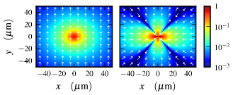
Figure 1: Flow fields of the model swimmers considered in our analytical and numerical calculations. In both plots, the swimmer is oriented upwards and the flow is normalized by the swimming speed. The arrows indicate velocity direction and the colors represent magnitude. (Left) Co-oriented model with $r^{-2}$ decay and (Right) stroke-averaged flow generated by a dipolar “pusher”. Parameters are those of Fig. 2.

We shall focus on two simplified models (see Fig. 1) that can be interpreted as contributions in a general multipole expansion of a flow field. Specifically, we will compare a co-oriented model 2010DuPuZaYe with trivial angular dependence

$$\boldsymbol{u}(\boldsymbol{x}|\Gamma^{\sigma})=(\kappa V)\;\left(\frac{\epsilon^{n}}{|\boldsymbol{R}^{\sigma}|^{n}+\lambda^{n}}\right)\hat{\boldsymbol{\Omega}}^{\sigma}\;,\qquad n\geq 1$$ (4a)

to a more realistic dipolar (or stresslet) flow field 1990PeKe

$$\boldsymbol{u}(\boldsymbol{x}|\Gamma^{\sigma})=(\kappa V)\left(\frac{\epsilon^{2}}{|\boldsymbol{R}^{\sigma}|^{2}+\lambda^{2}}\right)\left[3\left(\hat{\boldsymbol{\Omega}}^{\sigma}\hat{\boldsymbol{R}}^{\sigma}\right)^{2}-1\right]\hat{\boldsymbol{R}}^{\sigma}.$$ (4b)

In Eqs. (4), the vector $\boldsymbol{R}^{\sigma}(t):=\boldsymbol{X}^{\sigma}(t)-\boldsymbol{x}$ connects the swimmer and tracer position at time $t$, $\hat{\boldsymbol{R}}^{\sigma}(t):=\boldsymbol{R}^{\sigma}/|{\boldsymbol{R}}^{\sigma}|$ is the associated unit vector, and $\hat{\boldsymbol{\Omega}}^{\sigma}:=\hat{\boldsymbol{V}}^{\sigma}/V$ defines the swimmer’s orientation and swimming direction. The parameter $\epsilon$ characterizes the swimmer length scale, $\kappa$ is a dimensionless constant that relates the amplitude of the flow field to the swimmer speed, and $\lambda$ regularizes the singularity of the flow field at small distances. The co-oriented model (4a), due to its minimal angular dependence, is useful for pinpointing how the tracer statistics depend on the distance scaling of the flow field. For $n=1$, the scaling is equivalent to that of an “active” colloid or forced swimmer, whereas for $n\geq 2$ the scaling resembles that of various natural swimmers not subjected to an external force. In particular, the case $n=2$ allows us to ascertain the effects of the angular dependence of the flow field structure on tracer diffusion, by comparing against the more realistic dipolar model (4b). The latter is commonly considered as a simple stroke-averaged description for natural microswimmers 2009BaMa_PNAS ; 2002SiRa_PRL . As shown in Ref. 2010DuPuZaYe , stroke-averaged models are able to capture the most important aspects of the tracer dynamics on time scales longer than the swimming stroke of a microorganism.

II Results

We are interested in computing experimentally accessible, statistical properties of the tracer particles, such as their velocity PDF, correlation functions, and position PDF. These quantities are obtained by averaging suitably defined functions with respect to the $N$-swimmer distribution $\Phi_{N}=\prod_{\sigma}\Phi_{1}(\Gamma^{\sigma}_{0})$. A detailed description of the averaging procedure and a number of exact analytical results are given in the Supplementary Material, below we shall restrict ourselves to discussing the main results and their implications.

We begin by considering the equal-time velocity PDF and velocity autocorrelation function at a fixed point in the fluid. Since we are primarily interested in the swimmer contributions, we will focus on the deterministic limit $D_{0}=0$ first. The additive effect of thermal Brownian motion will be taken into account later, when we discuss the position statistics of the tracer. Considering a suspension of $N$ swimmers, confined by a spherical volume of radius $\Lambda$, the equal-time velocity PDF $\phi_{N,\Lambda}(\boldsymbol{v})$ and velocity autocorrelation function $C_{N,\Lambda}(t)$ of the flow field near the center of the container are formally defined by

$$\phi_{N,\Lambda}(\boldsymbol{v}):=\langle\delta(\boldsymbol{v}-\boldsymbol{u}_{N}(0,\boldsymbol{0}))\rangle,$$ (5a)

$$C_{N,\Lambda}(t):=\langle\boldsymbol{u}_{N}(t,\boldsymbol{0})\boldsymbol{u}_{N}(0,\boldsymbol{0})\rangle,$$ (5b)

where the average $\langle\;\cdot\;\rangle$ is taken with respect to the spatially uniform initial distribution of the swimmers. For the models (4), it is possible to determine $\phi_{N,\Lambda}$ and $C_{N,\Lambda}$ analytically.

II.1 Velocity PDF: Slow convergence of the central limit theorem for $\boldsymbol{n\geq 2}$

To elucidate the origin of the unusual velocity statistics in an active suspension, let us consider the tracer velocity PDF when there is a single swimmer present, $\phi_{1,\Lambda}(\boldsymbol{v})$. The tail of this function reflects large tracer velocities generated by close encounters with the swimmer. It is instructive to start with the (unphysical) limit $\lambda=0$, where the interaction diverges at short distances and there is no cutoff for large velocities. In this case, one readily finds from (5a) that asymptotically $\phi_{1,\Lambda}(0,\boldsymbol{v})\propto|\boldsymbol{v}|^{-(3+3/n)}$. This means that the variance of the probability distribution is finite for $n=1$, but infinite for $n\geq 2$. According to Eq. (2), the flow field due to $N$ swimmers is the sum of $N$ independent and identically distributed random variables. Hence, the central limit theorem predicts that, for $\lambda=0$ and $n=1$, the velocity distribution $\phi_{N,\Lambda}$ converges to a Gaussian in the large $N$ limit, whereas for $\lambda=0$ and $n\geq 2$ one expects non-Gaussian behavior due to the infinite variance of $\phi_{1,\Lambda}$.

For a real swimmer, the flow field is strongly increasing in the vicinity of the swimmer 2010DrEtAl_PRL ; 2010GuGo , but remains finite due to lubrication effects and nonzero swimmer size. This corresponds in our model to a positive value of $\lambda$. For $\lambda>0$, the variance of the one-swimmer PDF $\phi_{1,\Lambda}$ remains finite and, formally, the conditions for the central limit theorem are satisfied for all $n\geq 1$. However, for $n\geq 2$ the variance of $\phi_{1,\Lambda}$ remains very large and the convergence to a Gaussian limiting distribution is very slow. Our subsequent analysis demonstrates that the velocity PDF is more accurately described by a tempered Lévy-type distribution.

These statements are illustrated by Fig. 2, which shows velocity PDFs obtained numerically (symbols) and from analytical approximations (solid curves) for the co-oriented model with $n=1$ (A) and $n=2$ (B), and the dipolar model (C) at different swimmer volume fractions $\varphi:=N(\epsilon/\Lambda)^{3}$. As evident from Fig. 2 A, for $n=1$ the velocity PDF indeed converges rapidly to the Gaussian shape, in accordance with the central limit theorem. By contrast, for velocity fields decaying as $r^{-n}$ with $n\geq 2$, the convergence is surprisingly slow and one observes strongly non-Gaussian features at small filling fractions $\varphi$. The arrows highlight this regime, which shows a power-law dependence of the velocity distribution on the magnitude of the velocity, a signature of a Lévy distribution.

The remarkably slow convergence to the Gaussian central limit theorem prediction can be understood quantitatively by considering the characteristic function

$$\chi_{\phi}(\boldsymbol{q}):=\int\mathrm{d}^{3}v\;\exp(-i\boldsymbol{q}\boldsymbol{v})\;\phi(\boldsymbol{v})$$ (6)

of the velocity PDF (5a). A detailed analytical calculation (see Supplementary Material) shows that the exact result for $\chi_{\phi}(\boldsymbol{q})$ can be approximated by

$$\tilde{\chi}_{\phi}(|\boldsymbol{q}|)=\exp\{-[(c\;|\boldsymbol{q}|^{2}+\mu^{2})^{\alpha/2}-\mu^{\alpha}]\}.$$ (7)

This expression, which reduces to a Gaussian for $\alpha=2$, is of the tempered Lévy form, and gives rise to the following tracer velocity moments

$$\langle|\boldsymbol{v}|^{2}\rangle = 3\alpha c\;\mu^{\alpha-2},$$ (8a)

$$\langle|\boldsymbol{v}|^{4}\rangle = 15\alpha c^{2}\mu^{\alpha-4}\left[2+\alpha\left(\mu^{\alpha}-1\right)\right].$$ (8b)

By studying asymptotic behavior in the small cutoff limit $\lambda\to 0$ one finds that, for velocity fields $\boldsymbol{u}$ decaying as $r^{-n}$,

$$n=1\quad\Rightarrow\quad\alpha=2\;,\qquad\quad n\geq 2\quad\Rightarrow\quad\alpha=3/n.$$ (9)

This result confirms that for colloidal-type interactions with $n=1$ the velocity PDF is Gaussian, whereas for $n\geq 2$ deviations from Gaussianity occur in agreement with our numerical results of Fig. 2. In the limit $\mu=0$, Eq. (7) describes the family of Lévy stable distributions. These distributions arise from a generalized central limit theorem 1954GnKo relevant to random variables having an infinite variance. Specifically for $n=2$, one recovers the Holtsmark distribution that describes the statistics of the gravitational force acting on a star in a cluster 1943Ch and of the velocity field created by point vortices in turbulent flows 1984Ta .

However, for realistic non-singular flow fields, corresponding to finite values of $\lambda$, we generally have $\mu>0$. Specifically, by matching the exact velocity moments to those in Eq. (8), one finds that for the co-oriented model (4a) with $n=1$

$$c=\frac{1}{2}N\left(\frac{\epsilon}{\Lambda}\right)^{2}\ (\kappa V)^{2}\;\left[1+\ell+2\ell\log(\ell)\right]$$ (10)

at leading order in $\ell:=\lambda/\Lambda$, whereas for $n=2$

$$c = \frac{1}{3}\left(\frac{5\pi^{4}}{12}\right)^{1/3}\left(\kappa V\right)^{2}\varphi^{4/3},$$ (11a)

$$\ \mu = \left(\frac{10\pi}{3}\right)^{2/3}\left(\frac{\lambda}{\epsilon}\right)^{2}\varphi^{2/3}.$$ (11b)

For the dipolar model (4b), one obtains the same scaling of $(c,\mu)$ with $(\varphi,\lambda)$ as in Eq. (11) but with a slightly different numerical prefactor, yielding in the small cutoff limit $\lambda\to 0$

$$\langle|\boldsymbol{v}|^{2}\rangle = \frac{3\pi}{5}(\kappa V)^{2}\;\varphi\left(\frac{\epsilon}{\lambda}\right),$$ (12a)

$$\langle|\boldsymbol{v}|^{4}\rangle = \frac{9\pi}{70}(\kappa V)^{4}\;\varphi\left(\frac{\epsilon}{\lambda}\right)^{5}.$$ (12b)

Note that Eq. (10) suggests for colloidal-type flow fields with $\boldsymbol{u}\propto r^{-1}$ the appropriate thermodynamic limit is given by $N,\Lambda\to\infty$ such that $N/\Lambda^{2}=\mathit{const.}$, whereas we must fix $\varphi=\mathit{const.}$ if $\boldsymbol{u}\propto r^{-n},n\geq 2$. Furthermore, Eqs. (11b) and (12a) imply that $\mu\to 0$ and $\langle|\boldsymbol{v}|^{2}\rangle\to\infty$ for a vanishing regularization parameter $\lambda\to 0$. This illustrates that Lévy-type behavior becomes more prominent the more “singular” the velocity field in the vicinity of the swimmer.

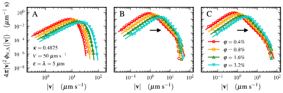
Figure 2: Velocity PDF of a tracer particle in the flow generated by different concentrations of swimmers. The solid curves are based on approximation (7), using the exact second and fourth moments of the velocity PDFs, as shown in the Supplementary Material. (A) For the co-oriented model (4a) with long-range hydrodynamics $n=1$, the velocity PDFs from simulations (symbols) converge rapidly to the Gaussian distribution predicted by the central limit theorem (solid curves), even at low volume fractions $\varphi\simeq 0.4\%$. (B) In contrast, for the co-oriented model with $n=2$, the central limit theorem convergence is very slow and the velocity distribution exhibits strongly non-Gaussian features at volume fractions similar to those realized by recent experiments 2009LeEtAl_Gold . (C) The velocity PDF for the dipolar swimmer model looks very similar to that of our co-oriented model (B), which means the angular dependence does not play an important role for the velocity distribution. Simulation parameters are given in A, the sample size is $4\times 10^{6}$ throughout.

The solid curves in Fig. 2 are based on approximation (7), using the exact second and fourth moments of the velocity PDFs, as given in the Supplementary Material. For $\boldsymbol{u}\propto r^{-2}$, the Gaussian prediction of the central limit theorem becomes accurate only at large volume fractions ($\varphi\gtrsim 25\%$). In the dilute regime $\varphi\ll 1$, the bulk of the probability comes from a Lévy stable distribution before it crosses over to quasi-Gaussian decay, reflected by the (truncated) power-law tails in Fig. 2 B and C. We may thus conclude that the fluid velocity in a dilute swimmer suspension is a biophysical realization of truncated Lévy-type random variables 1994Stanley .

II.2 Flow field autocorrelation

The similarity of Figs. 2 B and C suggests that the angular flow field structure is not important for the equal-time velocity distribution. By contrast, the velocity autocorrelation function $C_{N,\Lambda}(t)$ depends sensitively on the angular details, as illustrated in Fig. 3. For both our co-oriented model (4a) with $n=1,2$ and the dipolar model (4b), the function $C_{N,\Lambda}(t)$ can be determined analytically (see Supplementary Material). From the exact results, one finds that for $n=2$ in the thermodynamic limit at long times $t\gg\tau_{\epsilon}:=\epsilon/V$

$$C_{N,\Lambda}(t)\simeq\frac{3\pi^{2}}{4}\varphi\,(\kappa V)^{2}\,\,\left(\frac{\tau_{\epsilon}}{t}\right).$$ (13)

For comparison, the velocity autocorrelation function for dipolar swimmers can be approximated by

$$C_{N,\Lambda}(t)\simeq\varphi\;(\kappa V)^{2}\left(\frac{\epsilon}{\Lambda}\right)\frac{12}{5}\begin{cases}-1+\frac{1}{\ell_{*}}+\frac{3s^{2}}{7}-\frac{3s^{2}}{7\ell_{*}^{3}},&\ell_{*}\geq s,\\ -1-\frac{3\ell_{*}^{4}}{7s^{5}}+\frac{\ell_{*}^{2}}{s^{3}}+\frac{3s^{2}}{7},&\ell_{*}<s,\end{cases}$$ (14a)

where $$\ell_{*}:={4\ell}/{\pi} s:=tV/\Lambda<1$$ and . The approximation (14a), shown as the dotted line in Fig. 3, becomes exact at long times. In the thermodynamic limit, it reduces to

$$C_{N,\Lambda}(t)\simeq\varphi\;(\kappa V)^{2}\left(\frac{\epsilon}{\lambda}\right)\frac{3\pi}{5}\begin{cases}1-\frac{3t^{2}}{7\tau_{\lambda}^{2}},&t\leq\tau_{\lambda},\\ \frac{\tau_{\lambda}^{3}}{t^{3}}-\frac{3\tau_{\lambda}^{5}}{7t^{5}},&t>\tau_{\lambda},\end{cases}$$ (14b)

where $\tau_{\lambda}:=4\lambda/(\pi V)$. Note that Eq. (14b) predicts an asymptotic $t^{-3}$ decay, which is considerably faster than the $t^{-1}$ decay for the co-oriented model, cf. Eq. (13). This is due to the different angular structure of their respective flow fields. The excellent agreement between simulation data and the exact analytic curves (solid) in Fig. 3 also confirms the validity of our simulation scheme (see Numerical Methods in Supplementary Material).

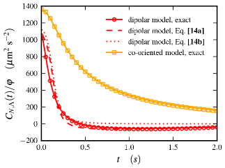
Figure 3: Due to the different flow topologies, the velocity autocorrelation function for dipolar swimmers (4b) decays faster than that for the co-oriented model (4a) with $n=2$. Solid curves indicate the exact analytic solution and symbols correspond to simulation data. Dotted and dashed curves illustrate respectively the long time approximation and its behavior in the thermodynamic limit. Parameters are those of Fig. 2.

II.3 Mean square displacement

Having discussed the velocity statistics, we next analyze the tracer displacements. To that end, we will focus on the practically more relevant dipolar swimmer case, and include the effects of thermal Brownian motion (so $D_{0}>0$). A first quantifier, that can be directly measured in experiments, is the mean square displacement $\langle\Delta[\boldsymbol{x}(t)]^{2}\rangle\simeq\langle\Delta[\boldsymbol{x}(t)]^{2}\rangle_{N}+6D_{0}t$. Assuming spatial homogeneity and spatially decaying correlations, the velocity autocorrelation function can be used to obtain an upper bound for the swimmer contribution

$$\langle\Delta[\boldsymbol{x}(t)]^{2}\rangle_{N} = \int_{0}^{t}\mathrm{d}\tau^{\prime}\int_{0}^{t}\mathrm{d}\tau\;\langle\boldsymbol{u}_{N}(\tau^{\prime},\boldsymbol{x}(\tau^{\prime}))\boldsymbol{u}_{N}(\tau,\boldsymbol{x}(\tau))\rangle$$ (15)

$$\leq \int_{0}^{t}\mathrm{d}\tau^{\prime}\int_{0}^{t}\mathrm{d}\tau\;\langle\boldsymbol{u}_{N}(\tau^{\prime},\boldsymbol{0})\boldsymbol{u}_{N}(\tau,\boldsymbol{0})\rangle.$$

Inserting the approximate result (14b), we find

$$\langle\Delta[\boldsymbol{x}(t)]^{2}\rangle_{N}\leq 6\,\varphi\;\kappa^{2}V\epsilon\;t\begin{cases}\frac{2t}{5\tau_{\lambda}}-\frac{t^{3}}{35\tau_{\lambda}^{3}},&t<\tau_{\lambda},\\ 1-\frac{\tau_{\lambda}}{t}+\frac{2\tau_{\lambda}^{2}}{5t^{2}}-\frac{\tau_{\lambda}^{4}}{35t^{4}},&t\geq\tau_{\lambda}.\end{cases}$$ (16)

Equation (16) implies that tracer diffusion due to the presence of dipolar swimmers is ballistic at short times $t\ll\tau_{\lambda}$ and normal at large times $t\gg\tau_{\lambda}$ (see Fig. 4). Qualitatively, the predicted linear growth $\langle\Delta[\boldsymbol{x}(t)]^{2}\rangle\propto t$ agrees with the experimental results of Leptos et al. 2009LeEtAl_Gold . Generally, the asymptotic diffusion constant will be of the form $D\simeq D_{0}+\nu\varphi\;\kappa^{2}V\epsilon$, where $\nu$ is a numerical prefactor of order unity that encodes spatial correlations neglected in Eq. (15).

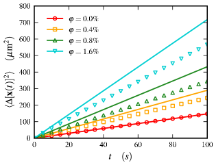
Figure 4: Mean square displacement at different volume fractions. Solid lines are analytic upper bounds, $6(D_{0}+\varphi\kappa^{2}V\epsilon)t\geq\langle\Delta[\boldsymbol{x}(t)]^{2}\rangle$, and symbols display the ensemble average from simulations. Parameters are those of Fig. 2.

II.4 Evolution of the position PDF

The spatial motion of a passive tracer in a fluctuating flow $\boldsymbol{u}(t,\boldsymbol{r})$ is described by the position PDF $P(t,\boldsymbol{r})=\langle\delta(\boldsymbol{r}-\boldsymbol{x}(t))\rangle$. For Gaussian fields, uniquely defined by the two-point correlation function $\langle u_{i}(t,\boldsymbol{r})u_{j}(t^{\prime},\boldsymbol{r}^{\prime})\rangle$, it is possible to characterize $P(t,\boldsymbol{r})$ analytically for some classes of trajectories $\boldsymbol{x}(t)$ 1995HaJu . However, our analysis above indicates that the statistics in an active suspension are neither $\delta$-correlated nor Gaussian, exhibiting features of Lévy processes.

Generally, the hierarchy of correlations in Lévy random fields is poorly understood 1994SaTa . It is therefore unclear how to adapt successful models of random advection by a Gaussian field 1994ShSi or, more generally, extend the understanding of colored Gaussian noise 1995HaJu to colored Lévy processes. These theoretical challenges make it very difficult, if not impossible, to construct an effective diffusion model that bridges the dynamics of $P(t,\boldsymbol{r})$ on all of the time scales. Partial theoretical insight can be gained, however, by considering the asymptotic short and long time behavior.

At short times $t\ll\tau_{\lambda}$, the position PDF combines ballistic transport from constant swimmer advection and diffusive spreading from thermal Brownian effects. For experimentally-relevant parameters 2009LeEtAl_Gold , normal diffusion is much stronger than the advection and, at these times, the dynamics of $P(t,\boldsymbol{r})$ are captured by the normal diffusion equation. If Brownian motion is neglected, we have $P(t,\boldsymbol{r})=t^{-3}\phi_{N,\Lambda}(\boldsymbol{r}/t)$ with $\phi_{N,\Lambda}(\boldsymbol{v})$ as the tempered Lévy velocity PDF. The resulting “ballistic” Lévy distribution is in good agreement with simulation data for $D_{0}=0$ at short times, see inset of Fig. 5 A.

For long times $t\gg\tau_{\lambda}$, after the correlations of the velocity field have vanished (typically after several seconds), we may interpret a tracer diffusing in an active suspension as a realization of an uncorrelated tempered Lévy process. Effectively, this corresponds to replacing $\boldsymbol{u}_{N}(t,\boldsymbol{r})$ from Eq. (1) with a $\delta$-correlated but non-Gaussian random function $\boldsymbol{\zeta}(t)$. To characterize the statistical properties of the swimmer-induced noise $\boldsymbol{\zeta}(t)$, we need to specify its characteristic functional $\mathcal{F}[t;\boldsymbol{k}(s)]$ 2009TouchetteCohen . Our earlier findings, that the asymptotic mean square displacement grows linearly in time and that the velocity field amplitudes follow a tempered Lévy stable distribution, suggest the functional form

$$\mathcal{F}[t;\boldsymbol{k}(s)]=\exp\left\{D_{\alpha}K^{\alpha}t-D_{\alpha}\int_{0}^{t}\mathrm{d}s\,[K^{2}+|\boldsymbol{k}(s)|^{2}]^{\alpha/2}\right\}.$$ (17)

Here, $D_{\alpha}$ is an anomalous diffusion coefficient of dimensions $\mathrm{m}^{\alpha}\mathrm{s}^{-1}$ and the regularization parameter $K$ has dimensions $\mathrm{m}^{-1}$. For $\alpha=2$, $\boldsymbol{\zeta}(t)$ reduces to Gaussian white noise. Using an approach similar to that of Ref. 2004Bu , the Fokker-Planck equation corresponding to Eq. (17) is found to be

$$\frac{\partial}{\partial t}P=\left\{D_{\alpha}\left[K^{\alpha}-(K^{2}-\nabla^{2})^{\alpha/2}\right]+D_{0}\nabla^{2}\right\}P,$$ (18)

where we also included the contribution from normal diffusion. In Fourier space, the solution of Eq. (18) reads

$$\hat{P}(t,\boldsymbol{k})=e^{D_{\alpha}\left[K^{\alpha}-(K^{2}+|\boldsymbol{k}|^{2})^{\alpha/2}\right]t-D_{0}|\boldsymbol{k}|^{2}t}.$$ (19)

Eq. (19) provides a good fit to the the long time simulation data in Figs. 5 C and 6, especially in the asymptotic regime. It is worth emphasizing that, although the motion of the tracers at long times is non-Gaussian and described by a fractional diffusion equation, the asymptotic mean square displacement exhibits normal growth, $\langle\Delta[\boldsymbol{x}(t)]^{2}\rangle\propto t$.

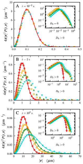
Figure 5: Radial position PDF of a tracer in a dilute suspension of dipolar swimmers at various times. Solid curves represent analytic forms of $P(t,\boldsymbol{r})$ and symbols illustrate histograms determined from simulations. Insets B and C show the same quantities on a log-log scale. Volume fractions and symbols are those of Fig. 4. Parameters are those of Fig. 2 with $D_{0}=0.245\ \mu\mathrm{m}^{2}\ \mathrm{s}^{-1}$. (A) Short time regime. At these times, Brownian motion effectively dominates constant advection for our choice of parameters. In the limit of no thermal noise (inset), the position PDF is the tempered Lévy velocity PDF $\phi_{N,\Lambda}(\boldsymbol{v})$ after a rescaling with $t$. (B) Transient behavior. This period corresponds to an intermediate decay of the velocity autocorrelation. (C) Asymptotic long time regime. Eventually, random advection from many low Reynolds number swimmers becomes equivalent to a tempered Lévy flight. The solution to the fractional diffusion equation (18) is matched against simulations by fitting its coefficients $D_{\alpha}$ and $K$, see also Fig. 6.

On intermediate time scales, when the velocity autocorrelations are already decaying, but still non-neglible due to their $t^{-3}$ scaling (see Fig. 3), the transient behavior of the position PDF can interpreted as a superposition of two distinct components: i) Quasi-ballistic tracer displacements, which are remnants of the short time dynamics and may dominate the tails of the tracer position distribution, and ii) fractional diffusive behavior due to the onset of tracer scattering by multiple swimmers. A quantitative comparison suggests that the measurements of tracer diffusion in Chlamydomonas suspensions by Leptos et al. 2009LeEtAl_Gold , who focused on the range $t\lesssim 2\ \mathrm{s}$, are exploring this intermediate regime.

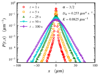
Figure 6: Time evolution of the marginal position PDF at a volume fraction $\varphi=1.6\%$. Solid curves represent Eq. (19) with fitted coefficients (shown only at long times) and symbols illustrate histograms determined from simulations. Parameters are those of Fig. 2 with $D_{0}=0.245\ \mu\mathrm{m}^{2}\ \mathrm{s}^{-1}$. At intermediate times $t\simeq 1\ \mathrm{s}$, our data resemble the measurements from Ref. 2009LeEtAl_Gold .

III Conclusions

Understanding the mixing and swimming strategies of algae and bacteria is essential for deciphering the driving factors behind evolution from unicellular to multicellular life 2010Drescher_PNAS . Recent experiments on tracer diffusion in dilute suspensions of unicellular biflagellate Chlamydomonas reinhardtii algae 2009LeEtAl_Gold have shown that microorganisms are able to significantly alter the flow statistics of the surrounding fluid, which may result in anomalous (non-Gaussian) diffusive transport of nutrients throughout the flow.

Here, we have developed a systematic theoretical description of anomalous tracer diffusion in dilute, active suspension. We demonstrated analytically and by means of GPU-based simulations that, depending on the distance scaling of microflows, qualitatively different flow field statistics can be expected. For colloidal-type flow fields that scale as $r^{-1}$ (due to the presence of an external force), the local velocity fluctuations in the fluid are predominantly Gaussian even at very small volume filling fraction, as expected from the classical central limit theorem. By contrast, flow fields that rise as $r^{-2}$ or faster in the vicinity of the swimmer will exhibit Lévy signatures. Very recent measurements by Rushkin et al. 2010Rushkin appear to confirm this prediction. When the statistics are non-Gaussian, our results show that the asymptotic convergence properties of velocity fluctuations in active swimmer suspensions are well-approximated by truncated Lévy random variables 1994Stanley .

With regard to experimental measurements, it is important to note that the tracer velocity is a well-defined observable only if thermal Brownian is negligible (corresponding to the limit $D_{0}=0$). Otherwise, the associated displacements over a time-interval $\Delta t$ contain a component that scales as $\sqrt{\Delta t}$. This fact must be taken into account, when one attempts to reconstruct velocity distributions from discretized trajectories: If thermal Brownian motion is a relevant contribution in the tracer dynamics, the measured distributions will vary depending on the choice of the discretization interval.

Our analysis further illustrates that, for homogeneous suspensions, the angular shape of the swimmer flow field is not important for the local velocity distribution, which is dominated by the radial flow structure. By contrast, the temporal decay of the velocity correlations sensitively depends on the angular topology of the individual swimmer flow fields. Specifically, our analytic calculations predicts that velocity autocorrelations in a dipolar swimmer suspension vanish algebraically as $t^{-3}$. This prediction could in principle be tested experimentally by monitoring the flow field at a fixed point in the fluid, using a setup similar to that in Ref. 2010Rushkin .

Finally, we propose that the asymptotic tracer dynamics can be approximated by a fractional diffusion equation with linearly growing asymptotic mean square displacement. It would be interesting to learn whether the fractional evolution of the tracer position distributions at long times can be confirmed experimentally. This, however, will require observational time spans that go substantially beyond those considered in Ref. 2009LeEtAl_Gold .

In conclusion, the correct and complete interpretation of experimental data requires an extension of Brownian motion beyond the currently existing approaches 1995HaJu ; 2000MeKl ; 2004MeKl . Although many challenging questions remain – in particular, regarding the consistent formulation of a generalized diffusion theory that combines Lévy-type fluctuations with time correlations – we hope that the present work provides a first step towards a better understanding of present and future experiments.

References

- (1) Hänggi, P & Marchesoni, F. (2005) 100 Years of Brownian Motion. Chaos 15, 026101.
- (2) Ingen-Housz, J. (1784) in Vermischte Schriften physisch-medicinischen Inhalts, ed. Molitor, N. C. (Christian Friderich Wappler, Wien).
- (3) Perrin, J. (1909) Mouvement Brownien et réalité moléculaire. Ann. Chim. Phys. 18, 5–114.
- (4) Sutherland, W. (1905) A dynamical theory of diffusion for non-electrolytes and the molecular mass of albumin. Philos. Mag 9, 781–785.
- (5) Einstein, A. (1905) Über die von der molekularkinetischen Theorie der Wärme geforderten Bewegung von in ruhenden Flüssigkeiten suspendierten Teilchen. Annalen der Physik und Chemie 17, 549–560.
- (6) Leptos, K. C, Guasto, J. S, Gollub, J. P, Pesci, A. I, & Goldstein, R. E. (2009) Dynamics of enhanced tracer diffusion in suspensions of swimming eukaryotic microorganisms. Phys. Rev. Lett. 103, 198103.
- (7) Purcell, E. M. (1977) Life at low Reynolds number. Am. J. Phys. 45, 3–11.
- (8) Han, Y, Alsayed, A. M, Nobili, M, Zhang, J, Lubensky, T. C, & Yodh, A. G. (2006) Brownian motion of an ellipsoid. Science 314, 626–630.
- (9) Li, T, Kheifets, S, Medellin, D, & Raizen, M. G. (2010) Measurement of the instantaneous velocity of a Brownian particle. Science 328, 1673–1675.
- (10) Polin, M, Tuval, I, Drescher, K, Gollub, J. P, & Goldstein, R. E. (2009) Chlamydomonas swims with two ”gears” in a eukaryotic version of run-and-tumble motion. Science 325, 487–490.
- (11) Drescher, K, Goldstein, R. E, & Tuval, I. (2010) Fidelity of adaptive phototaxis. Proc. Nat. Acad. Sci. 107, 11171–11176.
- (12) Sokolov, A, Apodacac, M. M, Grzybowskic, B. A, & Aranson, I. S. (2009) Swimming bacteria power microscopic gears. Proc. Nat. Acad. Sci. 107, 969–974.
- (13) Leonardo, R. D, Angelani, L, Dell’Arciprete, D, Ruocco, G, Iebba, V, Schippa, S, Conte, M. P, Mecarini, F, Angelis, F. D, & Fabrizio, E. D. (2010) Bacterial ratchet motors. Proc. Nat. Acad. Sci. 107, 9541–9545.
- (14) Wu, X.-L & Libchaber, A. (2000) Particle diffusion in a quasi-two-dimensional bacterial bath. Phys. Rev. Lett. 84, 3017.
- (15) Chen, D. T. N, Lau, A. W. C, Hough, L. A, Islam, M. F, Goulian, M, Lubensky, T. C, & Yodh, A. G. (2007) Fluctuations and rheology in active bacterial suspensions. Phys. Rev. Lett. 99, 148302.
- (16) Hernandez-Ortiz, J. P, Stoltz, C. G, & Graham, M. D. (2005) Transport and collective dynamics in suspensions of confined swimming particles. Phys. Rev. Lett. 95, 204501.
- (17) Underhill, P. T, Hernandez-Ortiz, J. P, & Graham, M. D. (2008) Diffusion and spatial correlations in suspensions of swimming particles. Phys. Rev. Lett. 100, 248101.
- (18) Metzler, R & Klafter, J. (2000) The random walk’s guide to anomalous diffusion: A fractional dynamics approach. Phys. Rep. 339, 1–77.
- (19) Metzler, R & Klafter, J. (2004) The restaurant at the end of the random walk: Recent developments in fractional dynamics descriptions of anomalous dynamical processes. J. Phys. A. 37, R161 –R208.
- (20) Mantegna, R. N & Stanley, H. E. (1994) Stochastic process with ultraslow convergence to a Gaussian: The truncated Lévy flight. Phys. Rev. Lett. 73, 2947–2949.
- (21) Drescher, K, Goldstein, R. E, Michel, N, Polin, M, & Tuval, I. (2010) Direct measurement of the flow field around swimming microorganisms. Phys. Rev. Lett. to appear.
- (22) Lauga, E & Powers, T. R. (2009) The hydrodynamics of swimming microorganisms. Rep. Prog. Phys. 72, 1–36.
- (23) Anderson, J. L. (1989) Colloid transport by interfacial forces. Ann. Rev. Fluid Mech. 21, 61–99.
- (24) Dunkel, J, Putz, V. B, Zaid, I. M, & Yeomans, J. M. (2010) Swimmer-tracer scattering at low Reynolds number. Soft Matter 6, 4268–4276.
- (25) Pedley, T. J & Kessler, J. O. (1990) A new continuum model for suspensions of gyrotactic microorganisms. J. Fluid Mech. 212, 155–182.
- (26) Baskaran, A & Marchetti, M. C. (2009) Statistical mechanics and hydrodynamics of bacterial suspensions. Proc. Nat. Acad. Sci. 106, 15567–15572.
- (27) Simha, R. A & Ramaswamy, S. (2002) Hydrodynamic fluctuations and instabilities in ordered suspensions of self-propelled particles. Phys. Rev. Lett. 89, 058101.
- (28) Guasto, J. S, Johnson, K. A, & Gollub, J. P. (2010) Oscillatory flows induced by microorganisms swimming in two-dimensions. arXiv:1008.2535.
- (29) Gnedenko, B. V & Kolmogorov, A. N. (1954) Limit Distributions for Sums of Independent Random Variables. (Addison-Wesley, Cambridge, MA).
- (30) Chandrasekhar, S. (1943) Stochastic problems in physics and astronomy. Rev. Mod. Phys. 15, 1–89.
- (31) Takayasu, H. (1984) Stable distribution and Lévy process in fractal turbulence. Prog. Theor. Phys. 72, 471–479.
- (32) Hänggi, P & Jung, P. (1995) Colored Noise in Dynamical Systems. Adv. Chem. Phys. 89, 239–326.
- (33) Samorodnitsky, G & Taqqu, M. S. (1994) Stable Non-Gaussian Random Processes: Stochastic Models with Infinite Variance. (Chapman & Hall, New York, NY).
- (34) Shraiman, B. I & Siggia, E. D. (1994) Lagrangian path-integrals and fluctuations in random flow. Phys. Rev. E 49, 2912–2927.
- (35) Touchette, H & Cohen, E. G. D. (2009) Anomalous fluctuation properties. Phys. Rev. E 80, 011114.
- (36) Budini, A. A & Cáceres, M. (2004) Functional characterization of generalized Langevin equations. J. Phys. A: Math. Gen. 37, 5959–5981.
- (37) Rushkin, I, Kantsler, V, & Goldstein, R. E. (2010) Fluid velocity fluctuations in a suspension of swimming protists. arXiv:1008.2770.