Robust graphical modeling of gene networks using classical and alternative $\bolds{t}$-distributions

Abstract

Graphical Gaussian models have proven to be useful tools for exploring network structures based on multivariate data. Applications to studies of gene expression have generated substantial interest in these models, and resulting recent progress includes the development of fitting methodology involving penalization of the likelihood function. In this paper we advocate the use of multivariate $t$-distributions for more robust inference of graphs. In particular, we demonstrate that penalized likelihood inference combined with an application of the EM algorithm provides a computationally efficient approach to model selection in the $t$-distribution case. We consider two versions of multivariate $t$-distributions, one of which requires the use of approximation techniques. For this distribution, we describe a Markov chain Monte Carlo EM algorithm based on a Gibbs sampler as well as a simple variational approximation that makes the resulting method feasible in large problems.

and T1Supported by NSF Grant DMS-07-46265. t2Supported by an Alfred P. Sloan Fellowship.

1 Introduction

Graphical Gaussian models have attracted a lot of recent interest. In these models an observed random vector $Y=(Y_{1},\dots,Y_{p})$ is assumed to follow a multivariate normal distribution $\mathcal{N}_{p}(\mu,\Sigma)$, where $\mu$ is the mean vector and $\Sigma$ the positive definite covariance matrix. Each model is associated with an undirected graph $G=(V,E)$ with vertex set $V=\{1,\dots,p\}$, and defined by requiring that for each nonedge $(j,k)\notin E$, the variables $Y_{j}$ and $Y_{k}$ are conditionally independent given all the remaining variables $Y_{\setminus\{j,k\}}$. Here, $\setminus\{j,k\}$ denotes the complement $V\setminus\{j,k\}$. Such pairwise conditional independence holds if and only if $\Sigma_{jk}^{-1}=0$; see Lauritzen (1996) for this fact and general background on graphical models. Therefore, inferring the graph corresponds to inferring the nonzero elements of $\Sigma^{-1}$.

Classical solutions to the model selection problem include constraint-based approaches that test the model-defining conditional independence constraints, and score-based searches that optimize a model score over a set of graphs. A review of this work can be found in Drton and Perlman (2007). Recently, however, penalized likelihood approaches based on the one-norm of the concentration matrix $\Sigma^{-1}$ have become increasingly popular. Meinshausen and Bühlmann 2006 proposed a method that uses lasso regressions of each variable $Y_{j}$ on the remaining variables $Y_{\setminus j}:=Y_{\setminus\{j\}}$. In subsequent work, Yuan and Lin (2007) and Banerjee, El Ghaoui and d’Aspremont (2008) discuss the computation of the exact solution to the convex optimization problem arising from the likelihood penalization. Finally, Friedman, Hastie and Tibshirani (2008) developed the graphical lasso (glasso), which is a computationally efficient algorithm that maximizes the penalized log-likelihood function through coordinate-descent. The theory that accompanies these algorithmic developments supplies high-dimensional consistency properties under assumptions of graph sparsity; see, for example, Ravikumar et al. (2009).

Inference of a graph can be significantly impacted, however, by deviations from normality. In particular, contamination of a handful of variables in a few experiments can lead to a drastically wrong graph. Applied work thus often proceeds by identifying and removing such experiments before data analysis, but such outlier screening can become difficult with large data sets. More importantly, removing entire experiments as outliers may discard useful information from the uncontaminated variables they may contain.

The existing literature on robust inference in graphical models is fairly limited. One line of work concerns constraint-based approaches and adopts robustified statistical tests [Kalisch and Bühlmann (2008)]. An approach for fitting the model associated with a given graph using a robustified likelihood function is described in Miyamura and Kano (2006). In some cases simple transformations of the data may be effective at minimizing the effect of outliers or contaminated data on a small scale. A normal quantile transformation, in particular, appears to be effective in many cases.

In this paper we extend the scope of robust inference by providing a tool for robust model selection that can be applied with highly multivariate data. We build upon the glasso of Friedman, Hastie and Tibshirani (2008), but model the data using multivariate $t$-distributions. Using the EM algorithm, the tlasso methods we propose are only slightly less computationally efficient than the glasso but cope rather well with contaminated data.

The paper is organized as follows. In Section 2 we review maximization of the penalized Gaussian log-likelihood function using the glasso. In Section 3 we introduce the classical multivariate $t$-distribution and describe maximization of the (unpenalized) log-likelihood using the EM algorithm. In Section 4 we combine the two techniques into the tlasso to maximize the penalized log-likelihood in the multivariate $t$ case. In Section 5 we introduce an alternative multivariate $t$-distribution and describe how inference can be done using stochastic and variational EM. In Section 6 we compare the glasso to our $t$-based methods on simulated data. Finally, in Section 7 we analyze two different gene expression data sets using the competing methods. Our findings are summarized in Section 8.

2 Graphical Gaussian models and the graphical lasso

Suppose we observe a sample of $n$ independent random vectors $Y_{1},\dots,Y_{n}\in\mathbb{R}^{p}$ that are distributed according to the multivariate normal distribution $\mathcal{N}_{p}(\mu,\Sigma)$. Likelihood inference about the covariance matrix $\Sigma$ is based on the log-likelihood function

$$\ell(\Sigma)=-\frac{np}{2}\log(2\pi)-\frac{n}{2}\log\det(\Sigma)-\frac{n}{2}\operatorname{tr}(S\Sigma^{-1}),\vspace*{-2pt}$$

where the empirical covariance matrix

$$S=(s_{jk})=\frac{1}{n}\sum_{i=1}^{n}(Y_{i}-\bar{Y})(Y_{i}-\bar{Y})^{T}\vspace*{-2pt}$$

is defined based on deviations from the sample mean $\bar{Y}$. Let $\Theta=(\theta_{jk})=\Sigma^{-1}$ denote the ($p\times p$)-concentration matrix. In penalized likelihood methods a one-norm penalty is added to the log-likelihood function, which effectively performs model selection because the resulting estimates of $\Theta$ may have entries that are exactly zero. Omitting irrelevant factors and constants, we are led to the problem of maximizing the function

$$\log\det(\Theta)-\operatorname{tr}(S\Theta)-\rho\|\Theta\|_{1}$$ (1)

over the cone of positive definite matrices, where $\|\Theta\|_{1}$ is the sum of the absolute values of the entries of $\Theta$. The multiplier $\rho$ is a positive tuning parameter. Larger values of $\rho$ lead to more entries of $\Theta$ being estimated as zero. Cross-validation or information criteria can be used to tune $\rho$.

The glasso is an iterative method for solving the convex optimization problem with the objective function in (1). Its updates operate on the covariance matrix $\Sigma$. In each step one row (and column) of the symmetric matrix $\Sigma$ is updated based on a partial maximization of (1) in which all but the considered row (and column) of $\Theta$ are held fixed. This partial maximization is solved via coordinate-descent as briefly reviewed next.

Partition off the last row and column of $\Sigma=(\sigma_{jk})$ and $S$ as

$$\Sigma=\pmatrix{\Sigma_{\setminus p,\setminus p}&\Sigma_{\setminus p,p}\vspace*{1pt}\cr\Sigma_{\setminus p,p}^{T}&\sigma_{pp}},\qquad S=\pmatrix{S_{\setminus p,\setminus p}&S_{\setminus p,p}\vspace*{1pt}\cr S_{\setminus p,p}^{T}&s_{pp}}.$$

Then, as shown in Banerjee, El Ghaoui and d’Aspremont (2008), partially maximizing $\Sigma_{\setminus p,p}$ with $\Sigma_{\setminus p,\setminus p}$ held fixed yields $\Sigma_{\setminus p,p}=\Sigma_{\setminus p,\setminus p}\beta^{*}$, where $\beta^{*}$ minimizes

$$\|(\Sigma_{\setminus p,\setminus p})^{1/2}\beta-(\Sigma_{\setminus p,\setminus p})^{-1/2}S_{\setminus p,p}\|^{2}+\rho\|\beta\|_{1}$$

with respect to $\beta\in\mathbb{R}^{p-1}$. The glasso finds $\beta^{*}$ by coordinate descent in each of the coordinates $j=1,\dots,p-1$, using the updates

$$\beta^{*}_{j}=\frac{T(s_{jp}-\sum_{k<p,k\neq j}\sigma_{kj}\beta^{*}_{k},\rho)}{\sigma_{jj}},$$

where $T(x,t)=\operatorname{sgn}(x)(|x|-t)_{+}$. The algorithm then cycles through the rows and columns of $\Sigma$ and $S$ until convergence. The diagonal elements are simply $\sigma_{pp}=s_{pp}+\rho$. See Friedman, Hastie and Tibshirani (2008) for more details on the method.

3 Graphical models based on the $t$-distribution

3.1 Classical multivariate $t$-distribution

The classical multivariate $t$-distribution $t_{p,\nu}(\mu,\Psi)$ on $\mathbb{R}^{p}$ has Lebesgue density

$$f_{\nu}(y;\mu,\Psi)=\frac{\Gamma((\nu+p)/2)|\Psi|^{-1/2}}{(\pi\nu)^{p/2}\Gamma(\nu/2)[1+\delta_{y}(\mu,\Psi)/\nu]^{(\nu+p)/2}}$$ (2)

with $\delta_{y}(\mu,\Psi)=(y-\mu)^{T}\Psi^{-1}(y-\mu)$ and $y\in\mathbb{R}^{p}$. The vector $\mu\in\mathbb{R}^{p}$ and the positive definite matrix $\Psi=(\psi_{jk})$ determine the first two moments of the distribution. If $Y\sim t_{p,\nu}(\mu,\Psi)$ with $\nu>2$ degrees of freedom, then the expectation is $\mathbb{E}[Y]=\mu$ and the covariance matrix is $\mathbb{V}[Y]=\nu/(\nu-2)\cdot\Psi$. From here on we will always assume $\nu>2$ for the covariance matrix to exist. For notational convenience and to illustrate the parallels with the Gaussian model, we define $\Theta=(\theta_{jk})=\Psi^{-1}$.

Figure 1: Graph representing the process generating a multivariate $t$-random vector $Y$ from a latent Gaussian random vector $X$ and a single latent Gamma-divisor.

If $X\sim\mathcal{N}_{p}(0,\Psi)$ is a multivariate normal random vector independent of the Gamma-random variable $\tau\sim\Gamma(\nu/2,\nu/2)$, then $Y=\mu+X/\sqrt{\tau}$ is distributed according to $t_{p,\nu}(\mu,\Psi)$; see Kotz and Nadarajah (2004), Chapter 1. This scale-mixture representation, illustrated in Figure 1, allows for easy sampling. It also clarifies how the use of $t$-distributions leads to more robust inference because extreme observations can arise from small values of $\tau$. An additional useful fact is that the conditional distribution of $\tau$ given $Y$ is again a Gamma-distribution, namely,

$$(\tau|Y)\sim\Gamma\biggl{(}\frac{\nu+p}{2},\frac{\nu+\delta_{Y}(\mu,\Psi)}{2}\biggr{)}.$$ (3)

Let $G=(V,E)$ be a graph with vertex set $V=\{1,\dots,p\}$. We define the associated graphical model for the $t$-distribution by requiring that $\theta_{jk}=0$ for indices $j\not=k$ corresponding to a nonedge $(j,k)\notin E$. This mimics the Gaussian model in that zero constraints are imposed on the inverse of the covariance matrix. However, in a $t$-distribution this no longer corresponds to conditional independence, and the density $f_{\nu}(y;\mu,\Psi)$ does not factor according to the graph. The conditional dependence manifests itself, in particular, in conditional variances in that even if $\theta_{jk}=0$,

$$\mathbb{V}[Y_{j}|Y_{\setminus j}]\not=\mathbb{V}\bigl{[}Y_{j}|Y_{\setminus\{j,k\}}\bigr{]}.\vspace*{-1pt}$$

For a simple illustration of this inequality, let $\Psi$ be a diagonal matrix. Then

$$\mathbb{V}[Y_{j}|Y_{\setminus j}]=\mathbb{E}[X_{j}^{2}/\tau|Y_{\setminus j}]=\frac{1}{\theta_{jj}}\cdot\mathbb{E}[\tau^{-1}|Y_{\setminus j}]=\frac{1}{\theta_{jj}}\cdot\frac{\nu+\delta_{Y_{\setminus j}}(\mu_{\setminus j},\Psi_{\setminus j,\setminus j})}{\nu+p-3},\vspace*{-2pt}$$

which can be shown by taking iterated conditional expectations, and using that

$$\mathbb{E}[X_{j}^{2}|Y_{\setminus j},\tau]=\mathbb{E}[X_{j}^{2}|X_{\setminus j},\tau]=\mathbb{V}[X_{j}|X_{\setminus j}]=\frac{1}{\theta_{jj}}\vspace*{-2pt}$$

and that $\tau$ given $Y_{\setminus j}$ has a Gamma-distribution; recall (3). Clearly, $\mathbb{V}[Y_{j}|Y_{\setminus j}]$ depends on all $Y_{k}$, $k\not=j$.

Despite the lack of conditional independence, the following property still holds (proved in the Appendix).

Proposition 1

Let $X\sim\mathcal{N}_{p}(0,\Theta^{-1})$, where $\theta_{jk}=0$ for pairs of indices $j\not=k$ that correspond to nonedges in the graph $G$. Let $\tau$ be independent of $X$ and follow any distribution on the positive real numbers with $\mathbb{E}[1/\tau]<\infty$ and define $Y=\mu+X/\sqrt{\tau}$. If two nodes $j$ and $k$ are separated by a set of nodes $C$ in $G$, then $Y_{j}$ and $Y_{k}$ are conditionally uncorrelated given $Y_{C}$.

The edges in the graph indicate the allowed conditional independencies in the latent Gaussian vector $X$. According to Proposition 1, however, we may also interpret the graph in terms of the observed variables $Y_{j}$. The zero conditional correlations entail that mean-square error optimal prediction of variable $Y_{j}$ can be based on the variables $Y_{k}$ that correspond to neighbors of the node $j$ in the graph, which is a very appealing property.

3.2 EM algorithm for estimation

The lack of density factorization properties complicates likelihood inference with $t$-distributions. However, the EM algorithm provides a way to circumvent this issue. Equipped with the normal-Gamma construction, we treat $\tau$ as a hidden variable and use that the conditional distribution of $Y$ given $\tau$ is $\mathcal{N}_{p}(\mu,\Psi/\tau)$. We now outline the EM algorithm for the $t$-distribution assuming the degrees of freedom $\nu$ to be known. If desired, $\nu$ could also be estimated in a line search that is best based on the actual $t$-likelihood [Liu and Rubin 1995].

Consider an $n$-sample $Y_{1},\dots,Y_{n}$ drawn from $t_{p,\nu}(\mu,\Psi)$. Let $\tau_{1},\dots,\tau_{n}$ be an associated sequence of hidden Gamma-random variables. Observation of the $\tau_{i}$ would lead to the following complete-data log-likelihood function for $\mu$ and $\Theta=\Psi^{-1}$:

$$\ell_{\mathrm{h}id}(\mu,\Theta|Y,\tau) \propto \frac{n}{2}\log\det(\Theta)-\frac{1}{2}\operatorname{tr}\Biggl{(}\Theta\sum_{i=1}^{n}\tau_{i}Y_{i}Y_{i}^{T}\Biggr{)}$$

$${}+\mu^{T}\Theta\sum_{i=1}^{n}\tau_{i}Y_{i}-\frac{1}{2}\mu^{T}\Theta\mu\sum_{i=1}^{n}\tau_{i},\vspace*{-2pt}$$

where, with some abuse, the symbol $\propto$ indicates that irrelevant additive constants are omitted. The complete-data sufficient statistics

$$S_{\tau}=\sum_{i=1}^{n}\tau_{i},\qquad S_{\tau Y}=\sum_{i=1}^{n}\tau_{i}Y_{i},\qquad S_{\tau YY}=\sum_{i=1}^{n}\tau_{i}Y_{i}Y_{i}^{T}\vspace*{-2pt}$$

are thus linear in $\tau$. We obtain the following EM algorithm for computing the maximum likelihood estimates of $\mu$ and $\Psi$:

E-step:

The E-step is simple because

$$\mathbb{E}[\tau|Y]=\frac{\nu+p}{\nu+\delta_{Y}(\mu,\Psi)}.\vspace*{-2pt}$$ (5)

Given current estimates $\mu^{(t)}$ and $\Psi^{(t)}$, we compute in the $(t+1)$st iteration

$$\tau_{i}^{(t+1)}=\frac{\nu+p}{\nu+\delta_{Y}(\mu^{(t)},\Psi^{(t)})}.\vspace*{-2pt}$$

M-step:

Calculate the updated estimates

$$\mu^{(t+1)} = \frac{\sum_{i=1}^{n}\tau_{i}^{(t+1)}Y_{i}}{\sum_{i=1}^{n}\tau_{i}^{(t+1)}},$$ (6)

$$\Psi^{(t+1)} = \frac{1}{n}\sum_{i=1}^{n}\tau_{i}^{(t+1)}\bigl{[}Y_{i}-\mu^{(t+1)}\bigr{]}\bigl{[}Y_{i}-\mu^{(t+1)}\bigr{]}^{T}.\vspace*{-1pt}$$ (7)

4 Penalized inference in $t$-distribution models

Model selection in graphical $t$-models can be performed, in principle, by any of the classical constraint- and score-based methods. In score-based searches through the set of all undirected graphs on $p$ nodes, however, each model would have to be refit using an iterative method such as the algorithm from Section 3.2. The penalized likelihood approach avoids this problem.

Like in the Gaussian case, we put a one-norm penalty on the elements of $\Theta$ and wish to maximize the penalized log-likelihood function

$$\ell_{\rho,\mathrm{obs}}(\mu,\Theta|Y)=\sum_{i=1}^{n}\log f_{\nu}(Y_{i};\mu,\Theta^{-1})-\rho\|\Theta\|_{1},$$ (8)

where $f_{\nu}$ is the $t$-density from (2). To achieve this, we will use a modified version of the EM algorithm taking into account the one-norm penalty.

We treat $\tau$ as missing data. In the E-step of our algorithm, we calculate the conditional expectation of the penalized complete-data log-likelihood

$$\ell_{\rho,\mathrm{hid}}(\mu,\Theta|Y,\tau)\propto\frac{n}{2}\log|\Theta|-\frac{n}{2}\operatorname{tr}(\Theta S_{\tau YY}(\mu))-\rho\|\Theta\|_{1}$$ (9)

with

$$S_{\tau YY}(\mu)=\frac{1}{n}\sum_{i=1}^{n}\tau_{i}(Y_{i}-\mu)(Y_{i}-\mu)^{T}.$$

Since $\ell_{\rho,\mathrm{hid}}(\mu,\Theta|Y,\tau)$ is again linear in $\tau$, the E-step takes the same form as in Section 3.2. Let $\mu^{(t)}$ and $\Theta^{(t)}$ be the estimates after the $t$th iteration, and $\tau_{i}^{(t+1)}$ the conditional expectation of $\tau_{i}$ calculated in the $(t+1)$st E-step. Then in the M-step of our algorithm we wish to maximize

$$\frac{n}{2}\log|\Theta|-\frac{n}{2}\operatorname{tr}\bigl{(}\Theta S_{\tau^{(t+1)}YY}(\mu)\bigr{)}-\rho\|\Theta\|_{1}$$

with respect to $\mu$ and $\Theta$. Differentiation with respect to $\mu$ yields $\mu^{(t+1)}$ from (6) for any value of $\Theta$. Therefore, $\Theta^{(t+1)}$ is found by maximizing

$$\frac{n}{2}\log|\Theta|-\frac{n}{2}\operatorname{tr}\bigl{(}\Theta S_{\tau^{(t+1)}YY}\bigl{(}\mu^{(t+1)}\bigr{)}\bigr{)}-\rho\|\Theta\|_{1}.$$ (10)

The quantity in (10), however, is exactly the objective function maximized by the glasso.

Iterating the E- and M-steps just described, we obtain what we call the tlasso algorithm. Since the one-norm penalty forces some elements of $\Theta$ exactly to zero, the tlasso performs model selection and parameter estimation in a way that is similar to structural EM algorithms [Friedman (1997)]. Convergence to a stationary point is guaranteed in the penalized version of the EM algorithm [McLachlan and Krishnan (1997), Chapter 1.6]; typically a local maximum is found. Note also that the maximized log-likelihood function is not concave, and so one finds oneself in the usual situation of not being able to give any guarantees about having obtained a global maximum.

5 Alternative model

5.1 Specification of the alternative $t$-model

The tlasso from Section 4 performs particularly well when a small fraction of the observations are contaminated (or otherwise extreme). In this case, these observations are downweighted in entirety, and the gain from reducing the effect of contaminated nodes outweighs the loss from throwing away good data from other nodes. In high-dimensional data sets, however, the contamination, or other deviation form normality, may be in small parts of many observations. Downweighting entire observations may then no longer achieve the desired results. We will demonstrate this later in simulations (see the bottom panel of Figure 4).

To handle the above situation better, we consider an alternative extension of the univariate $t$-distribution, illustrated in Figure 2. Instead of one divisor $\tau$ per $p$-variate observation, we draw $p$ divisors $\tau_{j}$. For $j=1,\ldots,p$, let $\tau_{j}\sim\Gamma(\nu/2,\nu/2)$ be independent of each other and of $X\sim\mathcal{N}_{p}(0,\Psi)$. We then say that the random vector $Y$ with coordinates $Y_{j}=\mu_{j}+X_{j}/\sqrt{\tau_{j}}$ follows an alternative multivariate $t$-distribution; in symbols $Y\sim t^{*}_{p,\nu}(\mu,\Psi)$.

Figure 2: Graph representing the process generating a $t^{*}$-random vector $Y$ from a latent Gaussian random vector $X$ and independent latent Gamma-divisors.

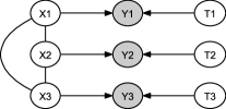
Unlike for the classical multivariate $t$-distribution, the covariance matrix $\mathbb{V}[Y]$ is no longer a constant multiple of $\Psi=(\psi_{jk})$ when $Y\sim t^{*}_{p,\nu}(\mu,\Psi)$. Clearly, the coordinate variances are still the same, namely,

$$\mathbb{V}[Y_{j}]=\frac{\nu}{\nu-2}\cdot\psi_{jj},$$

but the covariance between $Y_{j}$ and $Y_{k}$ with $j\not=k$ is now

$$\frac{\nu\Gamma((\nu-1)/2)^{2}}{2\Gamma(\nu/2)^{2}}\cdot\psi_{jk}\leq\frac{\nu}{\nu-2}\cdot\psi_{jk}.$$

The same matrix $\Psi$ thus implies smaller correlations (by the same constant multiple) in the $t^{*}$-distribution. This reduced dependence is not surprising in light of the fact that now different and independent divisors appear in the different coordinates. Despite the decrease in marginal correlations, the result of Proposition 1 does not hold for conditional correlations in the alternative model. That is, $\Psi^{-1}_{jk}=0$ does not imply $Y_{j}$ and $Y_{k}$ are conditionally uncorrelated given $Y_{\setminus\{j,k\}}$. Interpretation of the graph in the alternative model is thus limited to considering edges to represent the allowed conditional dependencies in the latent multivariate normal distribution.

Figure 3: Sample correlation of $Y_{1}$ and $Y_{2}$ for observations with $Y_{3}$ in a window of size 0.01.

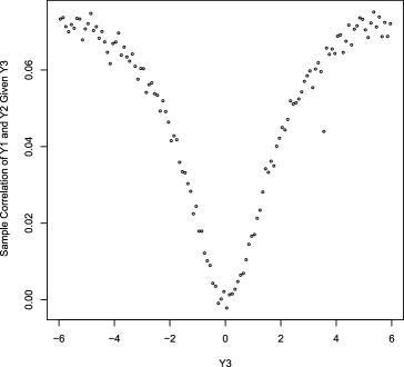
The following simulation confirms the result and illustrates the effect. We consider a $t^{*}_{3,3}(0,\Theta^{-1})$ distribution with

$$\Theta=\left[\matrix{1&0&-0.5\cr 0&1&-0.5\cr-0.5&-0.5&1\cr}\right]$$

and draw independent samples until we have 500,000 observations with $x<Y_{3}<x+0.01$ for $120$ values of $x$ in the range $(-6,6)$. The sample correlations of $Y_{1}$ and $Y_{2}$ given the varying values of $Y_{3}$ are shown in Figure 3.

5.2 Alternative tlasso

Inference in the alternative model presents some difficulties because the likelihood function is not available explicitly. The complete-data log-likelihood function $\ell^{*}_{\rho,\mathrm{hid}}(\mu,\Theta|Y,\tau)$, however, is simply the product of the evaluations of $p$ Gamma-densities ($\tau$ being a vector now) and a multivariate normal density. We can thus implement an EM-type procedure if we are able to compute the conditional expectation of $\ell^{*}_{\rho,\mathrm{hid}}(\mu,\Theta|Y,\tau)$ given $Y=(Y_{1},\dots,Y_{n})$. This time we treat the $p$ random variables $(\tau_{i1},\ldots,\tau_{ip})$ as hidden for each observation $i=1,\dots,n$. Unfortunately, the conditional expectation is intractable. It can be estimated, however, using Markov Chain Monte Carlo.

The complete-data log-likelihood function is equal to

$$\ell^{*}_{\rho,\mathrm{hid}}(\mu,\Theta,|Y,\tau)\propto\frac{n}{2}\log|\Theta|-\frac{n}{2}\operatorname{tr}(\Theta S^{*}_{\tau YY}(\mu))-\rho\|\Theta\|_{1},$$ (11)

where

$$S^{*}_{\tau YY}(\mu)=\frac{1}{n}\sum_{i=1}^{n}D\bigl{(}\sqrt{\tau_{i}}\bigr{)}(Y_{i}-\mu)(Y_{i}-\mu)^{T}D\bigl{(}\sqrt{\tau_{i}}\bigr{)}$$

and $D(\sqrt{\tau_{i}})$ is the diagonal matrix with $\sqrt{\tau_{i}}=\sqrt{\tau_{i1}},\ldots,\sqrt{\tau_{ip}}$ along the diagonal. The trace in (11) is linear in the entries of the matrix $\sqrt{\tau_{i}}\sqrt{\tau_{i}}^{T}$. A Gibbs sampler for estimating the conditional expectation of this matrix given $Y$ cycles through the coordinates indexed by $j=1,\ldots,p$ and draws, in its $m$th iteration, a number $\tau_{ij}^{(m)}$ from the conditional distribution of $\tau_{ij}$ given $(\tau_{i\setminus j},Y)$. This full conditional has density

$$f(\tau_{ij}|\tau_{i\setminus j},Y_{i})=C(\alpha,\beta,\gamma)\cdot\tau_{ij}^{\alpha-1}\exp\bigl{\{}-\tau_{ij}\beta-\sqrt{\tau_{ij}}\gamma\bigr{\}}$$ (12)

with

$$\hskip 30.0pt\alpha=\frac{\nu+1}{2},\qquad\beta=\frac{\nu+(Y_{ij}-\mu_{j})^{2}\theta_{jj}}{2},\qquad\gamma=(Y_{ij}-\mu_{j})\Theta_{j\setminus j}X_{i\setminus j},$$ (13)

and normalizing constant $C(\alpha,\beta,\gamma)$. This constant can always be expressed using hypergeometric functions, but, as we detail below, much simpler formulas can be obtained for the small integer degrees of freedom $\nu$ that are of interest in practice. The simpler formulas are obtained by partial integration.

From $\beta$ and $\gamma$ in (13), form the ratio $\gamma^{\prime}=\gamma/(2\sqrt{\beta})$. In order to sample from the distribution in (12), we may draw from

$$f_{\alpha,\gamma^{\prime}}(t)=C(\alpha,\gamma^{\prime})\cdot t^{\alpha-1}\exp\bigl{\{}-t-\sqrt{t}2\gamma^{\prime}\bigr{\}}$$ (14)

and divide the result by $\beta$. For our default of $\nu=3$, that is, $\alpha=2$, we thus need to sample from

$$f_{\gamma}(t)=C(\gamma)\cdot t\exp\bigl{\{}-t-\sqrt{t}2\gamma\bigr{\}}.$$ (15)

Writing $\Phi$ for the cumulative distribution function of the standard normal distribution, the normalizing constant becomes

$$1/C(\gamma)=1+\gamma^{2}-\gamma(2\gamma^{2}+3)\sqrt{\pi}\exp\{\gamma^{2}\}\bigl{(}1-\Phi\bigl{(}\gamma\sqrt{2}\bigr{)}\bigr{)}.$$ (16)

For $\gamma=0$, the density $f_{\gamma}(t)$ is a $\Gamma(2,1)$ density. For moderate $\gamma$, we are thus led to the following rejection sampling procedure to draw from $f_{\gamma}$.

Let $g_{\delta}$ be the density of a $\Gamma(2,\delta)$ distribution. Rejection sampling using the family of densities $g_{\delta}$ as instrumental densities proceeds by drawing a proposal $T\sim\Gamma(2,\delta)$ and a uniform random variable $U\sim\mathcal{U}(0,1)$ and either accept if $U\leq f(T)/(M_{\delta}g_{\delta}(T))$ or repeat the process until acceptance. Here, $M_{\delta}$ is a suitable multiplier such that $f(t)\leq M_{\delta}g_{\delta}(t)$ for all $t\geq 0$.

An important ingredient to the rejection sampler is the parameter $\delta$, which we choose as follows. In the case $\gamma<0$, the density $g_{\delta}$ has a heavier tail than $f$ provided that $\delta<1$. Focusing on the case $\alpha=2$, we have that for a given $\delta<1$ the smallest $M$ such that $f(t)\leq Mg_{\delta}(t)$ for all $t\geq 0$ is

$$M_{\delta}=C\cdot\frac{1}{\delta^{2}}\exp\biggl{\{}\frac{\gamma^{2}}{(1-\delta)}\biggr{\}}.$$

Varying $\delta$, the multiplier $M_{\delta}$ is minimized at

$$\delta=1+\frac{\gamma^{2}-\sqrt{\gamma^{4}+8\gamma^{2}}}{4}.$$

If $\gamma>0$, then setting $\delta=1$ yields a heavy enough tail and $M_{\delta}=C$.

The rejection sampling performs draws from the exact conditional distribution $f(\tau_{ij}|\tau_{i\setminus j},Y)$. We find it works very well for data with not too extreme contamination such as, for instance, in the original as well as bootstrap data from the application discussed in Section 7.2. When applied to data with very extreme observations $Y_{ij}$, however, one is faced with larger positive values of $\gamma$. In this case the instrumental densities $g_{\delta}$ provide a poor approximation to the target density $f_{\gamma}$, and the acceptance probabilities in the rejection sampling step become impractically low.

For $\gamma>1$, we thus use an alternative rejection procedure. Make the transformation $s=\sqrt{t}$. We then wish to sample from

$$h_{\gamma}(s)=2C(\gamma)\cdot s^{3}\exp\{-s^{2}-s2\gamma\}.$$

Any $\Gamma(\alpha,\delta)$ distribution has a heavier tail than the target distribution $h_{\gamma}(s)$. While it is not possible to find an analytical solution for the optimal $\alpha$ and $\delta$, letting $\alpha=1$ and $\delta=(\gamma+1)/2$ yields acceptance probabilities between $40\%$ and $50\%$ for most plausible values of $\gamma$. Since this alternative procedure will only be needed occasionally, these acceptance problems are adequate. Using this hybrid approach yields overall acceptance probabilities greater than $98\%$ for the data with extreme contamination described in Section 7.1.

Returning to the iterations of the overall sampler, we calculate $\sqrt{\tau_{i}}\sqrt{\tau_{i}}^{T}$ at the end of each cycle through the $p$ nodes, and then take the average over $M$ iterations. This solves the problem of carrying out one E-step, and we obtain the following stochastic penalized EM algorithm, which we call the Monte Carlo $t^{*}$-lasso (or $t^{*}_{\mathrm{M}C}$-lasso for short):

E-step:

Given current estimates $\mu^{(t)}$ and $\Psi^{(t)}$, compute ${(\sqrt{\tau_{i}}\sqrt{\tau_{i}}^{T})}^{(t+1)}$ by averaging the matrices obtained in some large number $M$ of Gibbs sampler iterations, as described above.

M-step:

Calculate the updated estimates

$$\mu_{j}^{(t+1)}=\frac{\sum_{i=1}^{n}\tau_{ij}^{(t+1)}Y_{ij}}{\sum_{i=1}^{n}\tau_{ij}^{(t+1)}}.$$

Use these and ${(\sqrt{\tau_{i}}\sqrt{\tau_{i}}^{T})}^{(t+1)}$ to compute the matrix $S^{*}_{\tau^{(t+1)}YY}(\mu^{(t+1)})$ to be plugged into the trace term in (11). Maximize the resulting penalized log-likelihood function using the glasso.

5.3 Variational approximation

The above Monte Carlo procedure loses much of the computational efficiency of the classical tlasso from Section 4, however, and can be prohibitively expensive for large $p$. For large problems, we turn instead to variational approximations of the conditional density $f(\tau_{i}|Y_{i})$ of the vector $\tau_{i}$ given the observed vector $Y_{i}$.

The variational approach proceeds by approximating the conditional density $f(\tau_{ij}|Y_{i})$ by a factoring distribution. In our context, however, it is easier to approximate the joint density $f(\tau_{i},Y_{i})=f(\tau_{i})f(Y_{i}|\tau_{i})$ instead. The first term is already in product form because we are assuming the individual divisor $\tau_{ij}$ to be independent in the model formulation, and the second term is the density of the multivariate normal distribution

$$\mathcal{N}_{p}\bigl{(}\mu,D\bigl{(}1/\sqrt{\tau_{i}}\bigr{)}\Theta^{-1}D\bigl{(}1/\sqrt{\tau_{i}}\bigr{)}\bigr{)}.$$

We approximate this normal distribution by a member of the set of multivariate normal distributions with diagonal covariance matrix. Application of this naive mean field procedure, that is, choosing a distribution by minimizing Kullback–Leibler divergence, leads to the approximating distribution

$$\mathcal{N}_{p}\bigl{(}\mu,D\bigl{(}1/\sqrt{\tau}\bigr{)}\bar{\Theta}^{-1}D\bigl{(}1/\sqrt{\tau}\bigr{)}\bigr{)},$$ (17)

where $\bar{\Theta}$ is the diagonal matrix with the same diagonal elements as $\Theta$ [Wainwright and Jordan (2008), Chapter 5]. Writing $q^{*}(Y|\tau)$ for the density of the distribution in (17), our approximation thus has the fully factoring form $q^{*}_{\tau_{i},Y_{i}}(\tau_{i},Y_{i})=f(\tau_{i})q^{*}(Y_{i}|\tau_{i})$. The resulting conditional distribution also factors as

$$q^{*}(\tau_{i}|Y_{i})=\prod_{j=1}^{p}g(\tau_{ij}|Y_{ij}),$$

where $g(\tau_{ij}|Y_{ij})$ is the density of the Gamma-distribution $\Gamma(\alpha_{ij},\beta_{ij})$, with its parameters corresponding to the quantities $\alpha$ and $\beta$ in (13).

In conclusion, the variational E-step consists of calculating, for each observation $Y_{i}$, the expectations

$$\mathbb{E}_{g}[\tau_{ij}|Y_{ij}]=\frac{\alpha_{ij}}{\beta_{ij}},\qquad\mathbb{E}_{g}\bigl{[}\sqrt{\tau_{ij}}|Y_{ij}\bigr{]}=\frac{\Gamma(\alpha_{ij}+1/2)}{\Gamma(\alpha_{ij})\sqrt{\beta_{ij}}},$$

and $\mathbb{E}[\sqrt{\tau_{j}}\sqrt{\tau_{k}}|Y_{i}]=\mathbb{E}_{g}[\sqrt{\tau_{j}}|Y_{ij}]\mathbb{E}_{g}[\sqrt{\tau_{k}}|Y_{ik}]$. These values are then substituted into (11). The M-step is the same as in the $t^{*}_{\mathrm{MC}}$-lasso.

The effect of the variational approximation is that the weight for node $j$ in observation $i$ is based solely on the squared deviation from the mean, $(Y_{ij}-\mu_{j})^{2}$ and the conditional variance $1/\theta_{jj}$. For a given deviation from the mean, the larger the conditional variance of the node, the smaller the weight given to that node in that observation. But unlike in the $t^{*}_{\mathrm{MC}}$-lasso, no consideration is given to deviation from the conditional mean of the node in question given the rest. Some relevant information is therefore not being used, but in our simulations the effect was not noticeable.

The resulting variational $t^{*}$-lasso ($t^{*}_{\mathrm{var}}$-lasso) is only slightly more expensive than the tlasso and, despite the relatively crude approximation in the variational E-step, performs well compared with the $t^{*}_{\mathrm{MC}}$-lasso. Because of this, we will use exclusively the $t^{*}_{\mathrm{var}}$-lasso when considering the alternative model in the simulations in the next section.

6 Simulation results

6.1 Procedure

We used simulated data to compare the three procedures glasso, tlasso and $t^{*}_{\mathrm{var}}$-lasso as follows. We generated a random $100\times 100$ sparse inverse covariance (or dispersion) matrix $\Theta$ according to the following procedure:

1. [(a)]

2. Choose each lower-triangular element of $\Theta$ independently to be $-1$, $0$ or $1$ with probability $1\%$, $98\%$ and $1\%$, respectively.

3. For $j>k$ set $\theta_{kj}=\theta_{jk}$.

4. Define $\theta_{kk}=1+h$ where $h$ is the number of nonzero elements in the $k$th row of $\Theta$.

The final step ensures a strictly diagonally dominant, and thus positive-definite matrix. To strengthen the partial correlations, we reduced the diagonal elements by a common factor. We made this factor as large as possible while maintaining positive-definiteness and stability for inversion. For these particular matrices, fixing a minimum eigenvalue of $0.6$ worked well.

We then generated $n=50$ observations from the $\mathcal{N}_{100}(0,\Theta^{-1})$ distribution and ran each of the three procedures with a range of values for the one-norm tuning parameter $\rho$. To compare how well the competing methods recovered the true edges, we drew ROC curves. We ran this whole process 250 times and then repeated the entire computation, drawing data from $t_{100,3}(0,\Theta^{-1})$ and then $t^{*}_{100,3}(0,\Theta^{-1})$ distributions.

Simulating from $t$-distributions produces extreme observations, but a more realistic setting might be one in which normal data is contaminated in some fashion. For instance, consider broken probes or misread observations in a large gene expression microarray. Suppose the contaminated data are not so extreme as to be manually screened or otherwise identified as obvious outliers. To simulate this phenomenon, we generate normal data as above, but randomly contaminated $2\%$ of the values with data generated from independent univariate $\mathcal{N}(\mu^{*},0.2)$ random variables, where $\mu^{*}$ is equal to $2.5$ times the largest diagonal element of $\Theta^{-1}$. These contaminated values will be similar in magnitude to the $2\%$ tail of the original $\mathcal{N}_{100}(0,\Theta^{-1})$ distribution and therefore difficult to identify.

Finally, we would like to compare our developed $t$-procedures with simpler approaches to robust inference. There are many ways to obtain robust estimates of the covariance matrix, but these usually require $n>p$. Instead we obtain a robust estimate for the marginal covariances and variances using the procedure of Kalisch and Bühlmann (2008). Since this is not guaranteed to result in a positive definite matrix, we add a constant, $c$, to the diagonal elements of the matrix, where $c$ is the minimum constant necessary to ensure the resulting matrix is nonnegative definite. We then use this robust estimate of the covariance matrix as input into the glasso and refer to this procedure as the robust glasso.

6.2 Results

Our tlasso and $t^{*}_{\mathrm{var}}$-lasso are computationally more expensive, since they call the glasso at each M-step. But in our simulations, the algorithms converge quickly. If we run through multiple increasing values of the tuning parameter $\rho$ for the one-norm penalty, it may take about $15$–$30$ EM iterations for the initial small value of $\rho$, but only 2 or 3 iterations for later values, as we can “warm start” at the previous output. But even in the initial run, two iterations typically lead to a drastic improvement (in the $t$ likelihood) over the glasso.

The only caveat is that the function being maximized by the tlasso methods is not guaranteed to be unimodal. We thus started in several places, and let the algorithm run for longer than probably necessary in practice. We did not observe drastically different results from different starting places. Nonetheless, since we are not guaranteed to find a global maximum, the statistical performances of the tlasso and $t^{*}_{\mathrm{var}}$-lasso may, in principle, be understated here (and, of course, the computational efficiency overstated).

Figure 4: ROC curves depicting the performances of the four methods under four different types of data. Each curve is an average over 250 simulations.

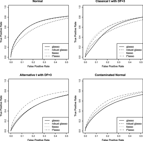
In the worst case scenario for our procedures relative to the glasso—when the data is normal and we assume $t$-distributions with $3$ degrees of freedom—almost no statistical efficiency is lost. In the numerous simulations we have run using normal data, the tlasso and glasso do an essentially equally good job of recovering the true graph (see Figure 4). The $t^{*}_{\mathrm{var}}$-lasso performs surprisingly well at small to moderate false discovery rates. The robust glasso is based on a less efficient estimator and does not perform as well as the other procedures.

For data generated from a classical $t$-distribution with $3$ degrees of freedom, the tlasso provides drastic improvement over the glasso at the low false positive rates that are of practical interest. The assumed normality and the occasional extreme observation lead to numerous false positives when using the glasso. Therefore, there is very little computational—and little or no statistical—downside to assuming $t$-distributions, but significant statistical upside. Interestingly, the $t^{*}_{\mathrm{var}}$-lasso performs about as well as the tlasso. The robust glasso outperforms the purely Gaussian procedure at low false positive rates, since it is less susceptible to the most extreme observations.

In the third case, with data generated from the alternative $t$-distribution with $3$ degrees of freedom, only the $t^{*}_{\mathrm{var}}$-lasso is able to recover useful information without substantial noise. The occasional large values are too extreme for the normal model to explain and downweighting entire observations, as is done by the tlasso, discards too much information when there are extreme values scattered throughout the data. The robust glasso offers only a small improvement over the glasso.

With the contaminated data, the $t^{*}_{\mathrm{var}}$-lasso does not perform as well in this case as it does with $t^{*}$ data. The extreme values are not downweighted as much and, thus, the signals are noisier. It still performs far better, however, than either of the other methods, and is able to recover valuable information in a case where manual screening of outliers would be very difficult. The robust glasso does not perform as well as the $t^{*}_{\mathrm{var}}$-lasso, but offers a clear improvement over the glasso and might be a useful alternative.

6.3 Notes on simulation

The simulations show that the tlasso performs very similarly to the glasso even with normal data. While one would expect a model based on the $t$-distribution to fare better with normal data than a normal model would with $t$ data, the fact that there is almost no statistical loss from the model misspecification is at first a bit surprising. The similarity of the results can be explained, however, by comparing the two procedures. In effect, the only difference is that the tlasso inputs a weighted sample covariance matrix into the glasso procedure; one can then think of the glasso as the tlasso with all weights set to one.

As noted in Section 3.2, these weights are the conditional expectations of $\tau$, which are, from equation (5),

$$\tau_{i}^{(t+1)}=\mathbb{E}[\tau_{i}|Y_{i}]=\frac{\hat{\nu}+p}{\hat{\nu}+\delta_{Y_{i}}(\mu^{(t)},\Psi^{(t)})},$$ (18)

where $\hat{\nu}$ is our estimate or assumption of the unknown degrees of freedom. If $Y\sim t_{p,\nu}(\mu,\Psi)$ and $\nu>4$, then $\delta_{Y}(\mu,\Psi)/p$ is distributed according to the $\mathcal{F}_{p,\nu}$ distribution [Kotz and Nadarajah (2004), Chapter 3]. Thus, starting with the true values of $\mu$ and $\psi$, the variance of the inverse weights is

$$\mathbb{V}\biggl{[}\frac{\hat{\nu}+\delta_{Y}(\mu,\Psi)}{\hat{\nu}+p}\biggr{]}=\frac{2p\nu^{2}(p+\nu-2)}{(\nu-2)^{2}(\nu-4)(\hat{\nu}+p)^{2}}.$$

For normal data (i.e., $\nu=\infty$), the variance is $2p/(\hat{\nu}+p)^{2}$ and goes to $0$ very quickly as $p$ gets large, no matter the assumed value of $\hat{\nu}$. If our current estimate of $\Theta$ is reasonably close to the true $\Theta$, then the observations will likely have very similar weights and the weighted covariance matrix will be very close to the sample covariance matrix. For $t$ data, the above variance tends to $2\nu^{2}/(\nu-2)^{2}(\nu-4)$ for large $p$; so no matter how many variables we have, the distribution of the inverse weights will have positive variance and the tlasso and glasso estimates are less likely to agree.

7 Gene expression data

7.1 Galactose utilization

We consider data from microarray experiments with yeast strands [Gasch et al. (2000)]. As in Drton and Richardson (2008), we limit this illustration to $8$ genes involved in galactose utilization. An assumption of normality is brought into question, in particular, by the fact that in $11$ out of $136$ experiments with data for all 8 genes, the measurements for 4 of the genes were abnormally large negative values. In order to assess the impact of this handful of outliers, we run each algorithm, adjusting the penalty term $\rho$ such that a graph with a given number of edges is inferred. Somewhat arbitrarily we focus on the top 9 edges. We do this once with all 136 experiments and then again excluding the $11$ potential outliers.

As seen in Figure 5, the glasso infers very different graphs, with only 3 edges in common. When the “outliers” are included, the glasso estimate in Figure 5(a) has the 4 nodes in question fully connected; when they are excluded, no edges among the 4 nodes are inferred. The tlasso does not exhibit this extreme behavior. As seen in Figure 5(b), it recovers almost the same graph in each case (7 out of 9 edges shared). When run with all the data, the $\tau$ estimate is very small (${\sim}0.04$) for each of the $11$ questionable observations compared with the average $\tau$ estimate of $1.2$. The graph in Figure 5(c) shows the results from the $t^{*}_{\mathrm{MC}}$-lasso which performs just as well as the tlasso. The $t^{*}_{\mathrm{var}}$-lasso also recovered 7 edges in both graphs (not shown) and infers relationships similar to those found by the $t^{*}_{\mathrm{MC}}$-lasso.

Figure 5: Top 9 recovered edges: (a) glasso, (b) tlasso, (c) $t^{*}_{\mathrm{MC}}$-lasso. Dashed edges were recovered only when including the outliers; dotted only when excluding them; solid in both cases.

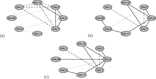
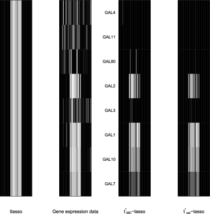
Figure 6 illustrates the flexibility of the weighting schemes of the various procedures. Both $t^{*}$ procedures downweight the 11 potential outliers observations for the 4 nodes in question, but not for the other nodes. Thus, the alternative version is able to extract information from the “uncontaminated” part of the $11$ observations while downweighting the rest. In this particular case, with 125 other observations, downweighting the outliers is of primary importance, and, thus, the increased flexibility of the $t^{*}_{\mathrm{MC}}$-lasso over the tlasso does not make much of a difference in the inferred graphs. This might not be the case with a higher contamination level.

7.2 Isoprenoid pathway

We next consider gene expression data for the isoprenoid pathways of Arabidopsis thaliana discussed in Wille et al. (2004). Gene expressions were measured in 118 Affymetrix microarrays for 39 genes. While the data set described in the above section had clear deviations from normality, the data described in this section has no obvious deviations that stand out in exploratory plots.

Figure 6: From left to right, inverse weights from tlasso, followed by normalized gene expression data, and inverse weights from $t^{*}_{\mathrm{MC}}$-lasso and $t^{*}_{\mathrm{var}}$-lasso. Rows correspond to genes and columns to observations. Lighter shades indicate larger values. The tlasso uses only one weight per observation and so must weight each gene the same. All plots show the same subset of data including $11$ potential outliers.

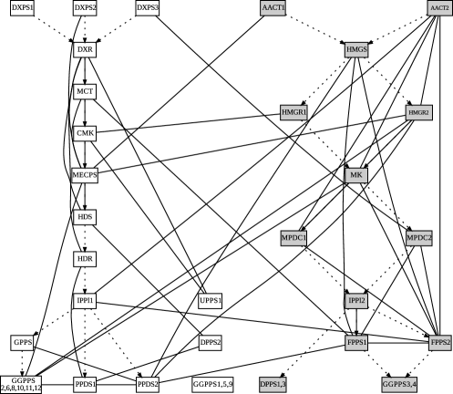
Two approaches were considered in Wille et al. (2004). The first (GGM1) fit a Gaussian graphical model using BIC and backward selection to obtain a network with 178 edges. This number was deemed too large for interpretation, and the authors considered instead only the 31 edges found in at least $80\%$ of bootstrapped samples. The second approach (GGM2) tests the conditional independence of each pair of genes given a third gene. An edge is drawn only if a test of conditional independence is rejected for each other gene in the network. This approach is advocated in the paper and appears to find a network with better biological interpretation. The graph is shown in Figure 7, where shaded nodes indicate the so-called MEP pathway.

Figure 7: A reproduction of the graph produced by Wille et al. Solid undirected edges are those found by the model selection procedure; dotted arrows show the metabolic pathway.

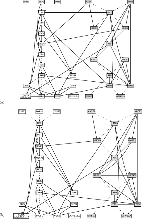
Our approach is modeled after GGM1. We used the $t^{*}_{\mathrm{var}}$-lasso and increasing values or $\rho$ to find a path of models to test. For each chosen model, we ran the $t^{*}_{\mathrm{var}}$-lasso again, but this time without penalty on the allowed edges. Since the $t^{*}$ likelihood is unavailable, we use leave-one-out cross-validation to find the model with the lowest mean squared prediction error. Since the exact conditionals from the alternative distribution are not available in explicit form, we perform the cross-validation as follows:

1. [(b)]

2. Estimate $\Theta$ using all but one observation.

3. In the remaining observation, estimate the values of the latent normal variables for all but one of the coordinates in the same manner as the variational E-step of Section 5.3.

4. Predict the remaining normal value.

5. Scale the normal value by the expectation of $1/\sqrt{\tau}$.

We remark that we also experimented with leaving out a larger fraction of the observations as suggested in the work of Shao (1993), but this led to similar conclusions in the present example.

The cross-validation procedure gave a network with 122 edges. To reduce to the graph size found by GGM2, we took 500 bootstrapped samples of the data, fixing the parameter $\rho$ found in cross-validation, and only included those edges found in more than $98.5\%$ of the samples. For comparison, we also ran the above procedure using the glasso, but keeping $98\%$ of the samples to obtain the same-sized graph.

We believe our procedure infers a graph that compares favorably (in terms of biological interpretation) with that found by GGM2. Like GGM2, we find a connection between AACT2 and the group MK, MPDC1 and FPPS2; GGM1 found AACT2 to be disconnected from the rest of the graph despite its high correlation with these three genes. In the MEP pathway, our approach and GGM2 find similar structure; compare Figures 7 and 8.

While our approach finds the key relationships identified in Wille et al., it achieves this with fewer “cross-talk” edges between the two pathways. The authors discuss plausible interpretations for such interactions between the pathways, but a graph with less cross-talk might be closer to the scientists’ original expectation (Figures 7 and 8). It is worth noting that the glasso procedure performs better than GGM1, with edge inclusion being far less sensitive to the particular bootstrapped sample. The glasso also finds the key relationships of GGM2. We also ran the tlasso, which gave results similar to the glasso and with the $t^{*}_{\mathrm{MC}}$-lasso, which behaved similar to the $t^{*}_{\mathrm{var}}$-lasso. We do not show these results here.

Figure 8: Graphs recovered by bootstrapping procedure with target graph size of 43 using (a) the glasso and (b) $t^{*}_{\mathrm{var}}$-lasso. The graph shows the key relationships identified previously, but with fewer “cross-talk” edges.

8 Discussion

Our proposed tlasso and $t^{*}_{\mathrm{var}}$-lasso algorithms are simple and effective methods for robust inference in graphical models. Only slightly more computationally expensive than the glasso, they can offer great gains in statistical efficiency. The alternative t distribution is more flexible than the classical $t$ and is generally preferred. We find that the simple variational E-step is an efficient way to estimate the graph in the alternative case, but also explored more sophisticated Monte Carlo approximations.

We assumed $\nu=3$ degrees of freedom in our various tlasso and $t^{*}$-lasso runs. As suggested in prior work on $t$-distribution models, estimation of the degrees of freedom can be done efficiently by a line search based on the observed log-likelihood function in the classical model.

Figure 9: The alternative $t$ model places an upper bound on the correlation between two variables. This bound increases with $\nu$, but is fairly restrictive for the small degrees of freedom we consider.

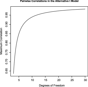
In the alternative model, the choice of $\nu$ puts an explicit upper bound on the maximum correlation between two variables, the upper bound increasing quickly with $\nu$ (see Figure 9). This makes inference of the degrees of freedom potentially more relevant than with the classical model, as an alternative model with small $\nu$ might not be a good fit for highly correlated variables. In order to select $\nu$, a line search based on the hidden log-likelihood function can be employed. For further flexibility, we may also allow the degrees of freedom to vary with each node. That is, we could let the divisors $\tau_{j}\sim\Gamma(\nu_{j}/2,\nu_{j}/2)$ be independent $\Gamma$-divisors with possible different degrees of freedom $\nu_{j}$. This leads to similar conditionals in the Gibbs sampler and the resulting procedure is thus no more complicated. Nevertheless, for the purposes of graph estimation, our experience and related literature suggest that not much is lost by considering only a few small values for the degrees of freedom. For instance, running the $t^{*}_{\mathrm{var}}$-lasso procedure in Section 7.2 using $\nu=5$ produces a very similar result with one additional cross-talk edge.

In the last section we used cross-validation to choose the one-norm tuning parameter $\rho$. The likelihood is not available explicitly for the $t^{*}$-distribution and so we cannot easily use information criteria for the $t^{*}$-lasso. Cross-validation often tends to pick more edges than is desirable, however, when the goal is inference of the graph and not optimal prediction. An interesting but potentially difficult problem for future research would be to develop rules for choosing $\rho$ that control an edge inclusion error rate; compare Banerjee, El Ghaoui and d’Aspremont (2008); Meinshausen and Bühlmann (2006).

Throughout the paper, we have penalized all the elements of $\Theta$. One alternative is to remove the penalty from the diagonal elements of $\Theta$, since we expect all these to be nonzero. This leads to smaller estimated partial correlations, and we found it to result in less stable behavior of the tlasso in the sense of the number of edges decreasing rather suddenly as $\rho$ increases.

Finally, we remark that other normal scale-mixture models could be treated in a similar fashion as the $t$-distribution models we considered in this paper. However, the use of $t$-distributions is particularly convenient in that it is rather robust to various types of misspecification, involves only the choice of the degrees of freedom parameters for the distribution of Gamma-divisors, and maintains good efficiency when data are Gaussian.

Appendix

Proof of Proposition 1 According to standard graphical model theory [Lauritzen (1996)], it suffices to show that $Y_{j}$ and $Y_{k}$ are conditionally uncorrelated given $Y_{V\setminus\{j,k\}}$. Partition $V$ into $a=\{j,k\}$ and $b=V\setminus\{j,k\}$. For a given value of $\tau$,

$$(Y_{a}|Y_{b},\tau)\sim N_{2}\bigl{(}\mu_{a}-\Theta_{a,a}^{-1}\Theta_{a,b}(Y_{b}-\mu_{b}),\Theta_{a,a}^{-1}/\tau\bigr{)}$$

and

$$(Y_{j}|Y_{k\,\cup\,b},\tau)\sim N\bigl{(}\mu_{i}-\theta_{jj}^{-1}\Theta_{j,k\,\cup\,b}(Y_{k\,\cup\,b}-\mu_{k\,\cup\,b}),\theta_{jj}^{-1}/\tau\bigr{)}.$$

Since $\theta_{jk}=0$,

$$\mathbb{E}[Y_{j}|Y_{k\,\cup\,b},\tau]=\mu_{j}-\theta_{jj}^{-1}\Theta_{j,b}(Y_{b}-\mu_{b})=\mathbb{E}[Y_{j}|Y_{b},\tau]$$

for any value of $\tau$. Therefore,

$$\mathbb{E}[Y_{j}|Y_{k\,\cup\,b}]=\mathbb{E}[\mathbb{E}[Y_{j}|Y_{k\,\cup\,b},\tau]|Y_{k\,\cup\,b}]=\mathbb{E}[\mathbb{E}[Y_{j}|Y_{b},\tau]|Y_{b}]=\mathbb{E}[Y_{j}|Y_{b}],$$

which implies that $Y_{j}$ and $Y_{k}$ are conditionally uncorrelated given $Y_{b}$.

References

- Banerjee, El Ghaoui and d’Aspremont (2008) {barticle}[author] \bauthor\bsnmBanerjee, \bfnmO.\binitsO., \bauthor\bsnmEl Ghaoui, \bfnmL.\binitsL. and \bauthor\bsnmd’Aspremont, \bfnmA.\binitsA. (\byear2008). \btitleModel selection through sparse maximum likelihood estimation for multivariate Gaussian or binary data. \bjournalJ. Mach. Learn. Res. \bvolume9 \bpages485–516. \MR2417243 \endbibitem
- Drton and Perlman (2007) {barticle}[author] \bauthor\bsnmDrton, \bfnmM.\binitsM. and \bauthor\bsnmPerlman, \bfnmD.\binitsD. (\byear2007). \btitleMultiple testing and error control in Gaussian graphical model selection. \bjournalStatist. Sci. \bvolume22 \bpages430–449. \MR2416818 \endbibitem
- Drton and Richardson (2008) {barticle}[author] \bauthor\bsnmDrton, \bfnmM.\binitsM. and \bauthor\bsnmRichardson, \bfnmT.\binitsT. (\byear2008). \btitleGraphical methods for efficient likelihood inference in Gaussian covariance models. \bjournalJ. Mach. Learn. Res. \bvolume9 \bpages893–914. \MR2417257 \endbibitem
- Friedman (1997) {binproceedings}[author] \bauthor\bsnmFriedman, \bfnmN.\binitsN. (\byear1997). \btitleLearning belief networks in the presence of missing values and hidden variables. In \bbooktitleProceedings of the Fourteenth International Conference on Machine Learning, \bpublisherNashville, TN. \endbibitem
- Friedman, Hastie and Tibshirani (2008) {barticle}[author] \bauthor\bsnmFriedman, \bfnmJ.\binitsJ., \bauthor\bsnmHastie, \bfnmT.\binitsT. and \bauthor\bsnmTibshirani, \bfnmR.\binitsR. (\byear2008). \btitleSparse inverse covariance estimation with the graphical lasso. \bjournalBiostatistics \bvolume9 \bpages432–441. \endbibitem
- Gasch et al. (2000) {barticle}[author] \bauthor\bsnmGasch, \bfnmA. P.\binitsA. P., \bauthor\bsnmSpellman, \bfnmP. T.\binitsP. T., \bauthor\bsnmKao, \bfnmC. M.\binitsC. M., \bauthor\bsnmCarmel-Harel, \bfnmO.\binitsO., \bauthor\bsnmEisen, \bfnmM. B.\binitsM. B., \bauthor\bsnmStorz, \bfnmS.\binitsG., \bauthor\bsnmBotstein, \bfnmD.\binitsD. and \bauthor\bsnmBrown, \bfnmP. O.\binitsP. O. (\byear2000). \btitleGenomic expression programs in the response of yeast cells to environmental changes. \bjournalMolecular Biology of the Cell \bvolume11 \bpages4241–4257. \endbibitem
- Kalisch and Bühlmann (2008) {barticle}[author] \bauthor\bsnmKalisch, \bfnmM.\binitsM. and \bauthor\bsnmBühlmann, \bfnmP.\binitsP. (\byear2008). \btitleRobustification of the PC-algorithm for directed acyclic graphs. \bjournalJ. Comput. Graph. Statist. \bvolume17 \bpages773–789. \MR2649066 \endbibitem
- Kotz and Nadarajah (2004) {bbook}[author] \bauthor\bsnmKotz, \bfnmS.\binitsS. and \bauthor\bsnmNadarajah, \bfnmS.\binitsS. (\byear2004). \btitleMultivariate -Distributions and Their Applications. \bpublisherCambridge Univ. Press, Cambridge. \MR2038227 \endbibitem
- Lauritzen (1996) {bbook}[author] \bauthor\bsnmLauritzen, \bfnmSteffen L.\binitsS. L. (\byear1996). \btitleGraphical Models. \bpublisherOxford Univ. Press, New York. \MR1419991 \endbibitem
- Liu and Rubin (1995) {barticle}[author] \bauthor\bsnmLiu, \bfnmC.\binitsC. and \bauthor\bsnmRubin, \bfnmD. B.\binitsD. B. (\byear1995). \btitleML estimation of the distribution using EM and its extensions, ECM and ECME. \bjournalStatist. Sinica \bvolume5 \bpages19–39. \MR1329287 \endbibitem
- McLachlan and Krishnan (1997) {bbook}[author] \bauthor\bsnmMcLachlan, \bfnmG.\binitsG. and \bauthor\bsnmKrishnan, \bfnmT.\binitsT. (\byear1997). \btitleThe EM Algorithm and Extensions. \bpublisherWiley, New York. \MR1417721 \endbibitem
- Meinshausen and Bühlmann (2006) {barticle}[author] \bauthor\bsnmMeinshausen, \bfnmN.\binitsN. and \bauthor\bsnmBühlmann, \bfnmP.\binitsP. (\byear2006). \btitleHigh dimensional graphs and variable selection with the lasso. \bjournalAnn. Statist. \bvolume34 \bpages1436–1462. \MR2278363 \endbibitem
- Miyamura and Kano (2006) {barticle}[author] \bauthor\bsnmMiyamura, \bfnmM.\binitsM. and \bauthor\bsnmKano, \bfnmY.\binitsY. (\byear2006). \btitleRobust Gaussian graphical modeling. \bjournalJ. Multivariate Anal. \bvolume97 \bpages1525–1550. \MR2275418 \endbibitem
- Ravikumar et al. (2009) {bincollection}[author] \bauthor\bsnmRavikumar, \bfnmP.\binitsP., \bauthor\bsnmRaskutti, \bfnmG.\binitsG., \bauthor\bsnmWainwright, \bfnmM. J.\binitsM. J. and \bauthor\bsnmYu, \bfnmB.\binitsB. (\byear2009). \btitleModel selection in Gaussian graphical models: High-dimensional consistency of -regularized MLE. In \bbooktitleAdvances in Neural Information Processing Systems (NIPS) (\beditorD. Koller, D. Schuurmans, Y. Bengio and L. Botto, eds.) \bvolume21 \bpages1329–1336. \endbibitem
- Shao (1993) {barticle}[author] \bauthor\bsnmShao, \bfnmJ.\binitsJ. (\byear1993). \btitleLinear model selection by cross-validation. \bjournalJ. Amer. Statist. Assoc. \bvolume88 \bpages486–494. \MR1224373 \endbibitem
- Wainwright and Jordan (2008) {barticle}[author] \bauthor\bsnmWainwright, \bfnmM. J.\binitsM. J. and \bauthor\bsnmJordan, \bfnmM. I.\binitsM. I. (\byear2008). \btitleGraphical models, exponential families, and variational inference. \bjournalFoundations and Trends\tsup® in Machine Learning \bvolume1 \bpages1–305. \endbibitem
- Wille et al. (2004) {barticle}[author] \bauthor\bsnmWille, \bfnmAnja\binitsA., \bauthor\bsnmZimmermann, \bfnmPhilip\binitsP., \bauthor\bsnmVranova, \bfnmEva\binitsE., \bauthor\bsnmFurholz, \bfnmAndreas\binitsA., \bauthor\bsnmLaule, \bfnmOliver\binitsO., \bauthor\bsnmBleuler, \bfnmStefan\binitsS., \bauthor\bsnmHennig, \bfnmLars\binitsL., \bauthor\bsnmPrelic, \bfnmAmela\binitsA., \bauthor\bparticlevon \bsnmRohr, \bfnmPeter\binitsP., \bauthor\bsnmThiele, \bfnmLothar\binitsL., \bauthor\bsnmZitzler, \bfnmEckart\binitsE., \bauthor\bsnmGruissem, \bfnmWilhelm\binitsW. and \bauthor\bsnmBühlmann, \bfnmPeter\binitsP. (\byear2004). \btitleSparse graphical Gaussian modeling of the isoprenoid gene network in Arabidopsis thaliana. \bjournalGenome Biology \bvolume5 \bpagesR92.
- Yuan and Lin (2007) {barticle}[author] \bauthor\bsnmYuan, \bfnmM.\binitsM. and \bauthor\bsnmLin, \bfnmY.\binitsY. (\byear2007). \btitleModel selection and estimation in the Gaussian graphical model. \bjournalBiometrika \bvolume94 \bpages19–35. \MR2367824 \endbibitem