Chirikov Diffusion in the Asteroidal Three-Body Resonance $\left(5,-2,-2\right)$

Abstract

The theory of diffusion in many-dimensional Hamiltonian system is applied to asteroidal dynamics. The general formulations developed by Chirikov is applied to the Nesvorný-Morbidelli analytic model of three-body (three-orbit) mean-motion resonances (Jupiter-Saturn-asteroid system). In particular, we investigate the diffusion along and across the separatrices of the $\left(5,-2,-2\right)$ resonance of the (490) Veritas asteroidal family and their relationship to diffusion in semi-major axis and eccentricity. The estimations of diffusion were obtained using the Melnikov integral, a Hadjidemetriou-type sympletic map and numerical integrations for times up to $10^{8}$ years.

1 Introduction

The application of chaotic dynamics concepts to asteroidal dynamics led to the understanding of the main structural characteristics of asteroids distribution within the solar system. It was verified that chaotic region are generally devoid of larger asteroids while, in contrast, regular regions exhibit a great number of them (see for instance, Berry 1978, Wisdom 1982, Dermott and Murray 1983, Hadjidemetriou and Ichtiaroglou 1984, Ferraz-Mello et al. 1997, Tsiganis et al. 2002b, Knežević 2004, Varvoglis 2004) It was soon accepted that chaos was related inevitably to instability, which may be local or global. Subsequent investigations searched for initial conditions leading to instabilities in relatively short time. In many applications, the determination of Lyapunov exponent on a grid of initial conditions was used to get quantitative informations on stability. The inverse of the largest Lyapunov exponent, called Lyapunov time, should be in some way linked to the characteristic time for the onset of chaos (Morbidelli and Froeschlé, 1996).

However, some investigations have shown that many asteroids exhibit intermediary behavior between chaos and regularity. The first registered case was the asteroid (522) Helga (Milani and Nobili, 1992). This asteroid was in chaotic orbit with a Lyapunov time inch shorter than the age of the solar system, but it exhibited a long period stability. No significant evolution was observed in the orbital elements of (522) Helga for times up to one thousand times its Lyapunov time. Since then, other asteroids have been shown to have Lyapunov times much shorter than the stability times unraveled by simulations (e.g., Trojans, cf. Milani 1993). Currently, this behavior is known in literature as stable chaos (Milani et al. 1997, Tsiganis et al. 2002a, Tsiganis et al. 2002b). Indeed, there is strong evidence that local instability does not mean chaotic diffusion, in the sense that nothing can be said about how much global or local integrals (or orbital elements) could change in a chaotic domain, even when a linear stability analysis shows rather short Lyapunov times (see Giordano and Cincotta, 2004, Cincotta and Giordano 2008).

Nesvorný and Morbidelli (1998, 1999) demonstrated that one source of stable chaos is related with three-body (three-orbit) mean-motion resonances (Jupiter-Saturn-asteroid system). They observed that asteroids in these resonances exhibit a slow diffusion in eccentricity and inclination, but no diffusion in the semi-major axis. According to the estimates of Nesvorný and Morbidelli (1998), about 1500 among the first numbered asteroids are affected by three-body mean-motion resonances.

The three-body mean-motion resonances are very narrow since they appear at second order in planetary masses, their typical width being $\sim 10^{-3}$ AU, but they are much more dense (in phase space) than standard two-body mean-motion resonances of similar size. Nesvorný and Morbidelli (1999) developed a detailed model for the three-body mean-motion resonance and presented analytical and numerical evidence that most of them exhibit a highly chaotic dynamics (at moderate-to-low-eccentricities) which may be explained in terms of an overlap of their associated multiplets. By multiplet, we refer to all resonances for which the time-derivative of the resonant angle, $\sigma_{p,p_{J},p_{S}}$, satisfies

$$\dot{\sigma}_{p,p_{J},p_{S}}=m_{J}\dot{\lambda}_{J}+m_{S}\dot{\lambda}_{S}+m\dot{\lambda}+p\dot{\varpi}+p_{J}\dot{\varpi}_{J}+p_{S}\dot{\varpi}_{S}\simeq 0,$$ (1)

for given $\left(m_{J},m_{S},m\right)\in\mathbb{Z}^{3}/\{0\}$. In (1) the $\lambda$’s and $\varpi$’s denote, as usual, the mean longitudes and perihelion longitudes, respectively; $\left(p,p_{J},p_{S}\right)\in\mathbb{Z}^{3}$ are integers such that $\sum_{i}\left(m_{i}+p_{i}\right)=0$ for i ranging over three bodies (Jupiter, Saturn and the asteroid).

We will be dealing in this paper with the case $\left(m_{J},m_{S},m\right)=\left(5,-2,-2\right)$. This three-body resonance seems to dominate the dynamics of, for instance, the asteroids (3460) Ashkova, (2039) Payne-Gaposchkin and (490) Veritas (see Nesvorný and Morbidelli 1999). In the case of the first two of those asteroids (with relatively large eccentricity, $\sim 0.15-0.20$), their behavior looks regular over comparatively long time-scales (typically $\sim 1-10\times 10^{3}$ years) while in case of (490) Veritas (with eccentricity, $\sim 0.06$) its dynamics looks rather chaotic over similar time-scales. The determination of the age of (490) Veritas family has been the concern of some authors who studied stable chaos (Milani and Farinella 1994, Knežević 1999, Knežević et al. 2002, Knežević 2003, Knežević et al. 2004, Tsiganis et al. 2007, Knežević 2007, Novaković et al. 2009).

Herein, we investigate chaotic diffusion along (and also across) the above mentioned three-body mean-motion resonance by means of a classical diffusion approach. We use (partially) the formulations given by Chirikov (1979). That formulation are developed to study specifically Arnold diffusion or some kind of diffusion that geometrically resembles it initially called Fast-Arnold diffusion by Chirikov and Vecheslavov (1989, 1993), as well as the so called modulational diffusion (Chirikov et. al, 1985). However, although from the purely mathematical point of view several restrictions should be imposed, there are many unsolved aspects regarding general phase space diffusion (see for instance Lochak 1999, Cincotta 2002, Cincotta and Giordano 2008).

The structure of the Hamiltonian used by Chirikov in his first formulation is similar to the Hamiltonians obtained with the perturbations theories of Celestial Mechanics. In particular, the Hamiltonians of analytic models of the three-body mean-motion resonances are directly adaptable, with some restrictions, to Chirikov’s formulations.

Let us mention that some progress has been done in the study of Arnold diffusion, particularly when applied to simple dynamical systems, like maps, the latest ones are for instance, the works of Guzzo et. al (2009a),(2009b), Lega (2009). However the link between strictly Arnold diffusion and general diffusion in phase space is still an open matter. Indeed, Arnold diffusion requires a rather small perturbation, when the measure of the regular component of phase space is close to one. Thus, as far as we know, almost all investigations regarding Arnold diffusion involves relatively simple dynamical systems like quasi–integrable maps. In more real systems, like the one investigated in this paper, the scenario is much more complex in the sense that the domain of the three body resonance is almost completely chaotic.

Finally, this work is justified by the fact that an application of all those theories to real astronomical models is still needed.

In Sect. 2, we summarize the general problem of computation of the diffusion rate along the resonance and we discuss the limitations and difficulties to follow Chirikov approach in case of this particular three-body mean-motion resonance. Section 3 is devoted to the resonant Hamiltonian (given in Nesvorný and Morbidelli (1999)) and its application to the $\left(5,-2,-2\right)$ resonance. In Sect. 4, we construct the simplified (or two-resonance) and complete (or three-resonance) numerical models used in our investigations. Moreover, informations about the algorithms and initial conditions used for numerical integrations and the procedure for estimation of the diffusion are also considered in this section. In Sect. 5, we discuss the numerical results on diffusion in the $\left(5,-2,-2\right)$ resonance. In this application of the Chirikov theory, we are concerned with the role of the perturbing resonances in the diffusion across and along the $\left(5,-2,-2\right)$ resonance and their relationship to diffusion in semi-major axis and eccentricity. Finally, in Sect. 6, we investigate the behavior of the asymptotic diffusion decreasing the intensity of the perturbations in the $\left(5,-2,-2\right)$ resonance. In this case, we are interested in the study of the diffusion under the action of an arbitrarily weak perturbation considering scenarios close to that of the Arnold diffusion.

2 Chirikov’s Diffusion Theory

In this section we give Chirikov’s (1979) as well as Cincotta’s (2002) description of diffusion theory in phase space in order to provide a self-consistent presentation of the subject. Since most of the results and discussions given here are included in at least these two reviews, we just address the basic theoretical aspects.

Let us consider a Hamiltonian system having several periodic perturbations that can create resonances. The initial conditions are chosen such that the system is in the domain of a main resonance, called guiding resonance. The term of perturbation corresponding to the guiding resonance is separated from the others, which will be called of perturbing resonances. The Hamiltonian has the following form

$$H=H_{0}\left(\mathbf{I}\right)+\epsilon V_{G}\left(\mathbf{I}\right)\cos\left(\mathbf{m}_{G}\cdot\boldsymbol{\theta}\right)+\epsilon V\left(\mathbf{I},\boldsymbol{\theta}\right),$$ (2)

with

$$\epsilon V=\epsilon\sum_{\mathbf{m}\neq\mathbf{m}_{G}}V_{\mathbf{m}}\left(\mathbf{I}\right)\cos\left(\mathbf{m}\cdot\boldsymbol{\theta}\right),$$ (3)

where $V_{G}$ and $\mathbf{\mathbf{m}}_{G}$ are, respectively, the amplitude and resonant vector of the guiding resonance, $V_{\mathbf{m}}$ and $\mathbf{m}$ are, respectively, the amplitude and resonant vectors of perturbing resonances. Here $\left(\mathbf{I},\boldsymbol{\theta}\right)$ are the usual N-dimensional action-angle coordinates for the unperturbed Hamiltonian $H_{0}\left(N\geq 3\right)$, the vectors $\mathbf{m}_{G}$, $\mathbf{m}\in\mathbb{Z}^{N}/\{0\}$ and $V_{G}$, $V_{\mathbf{m}}$ are real functions. The small parameter perturbation, $\epsilon$, is a real number such that $\epsilon\ll 1$. The resonance condition is fixed by

$$S\left(\mathbf{I}^{r}\right)\mathbf{=}\mathbf{m}_{G}\cdot\mathbf{\boldsymbol{\omega}}\left(\mathbf{I}^{r}\right)=0.$$ (4)

The surface $S\left(\mathbf{I}^{r}\right)=0$ in the action space, is called resonant surface.

2.1 Dynamics of the guiding resonance in the actions space

Let us first consider the simple case of one single resonance, that is, let us assume that all $V_{\mathbf{m}}=0$ for $\mathbf{m}\neq\mathbf{m}_{G}$, and we chose initial conditions close to the separatrix of the guiding resonance. In the $\boldsymbol{\omega}$-space, the resonance condition $\mathbf{m}_{G}\cdot\boldsymbol{\omega}^{r}=0$ has a very simple structure, just a $\left(N-1\right)$-dimensional plane the normal of which is the resonant vector $\mathbf{m}_{G}$. In the $\mathbf{I}$-space, $\mathbf{m}_{G}\cdot\boldsymbol{\omega}^{r}=0$ leads to the $\left(N-1\right)$-dimensional resonant surface $S\left(\mathbf{I}^{r}\right)=0$, whose local normal at the point $\mathbf{I}=\mathbf{I}^{r}$ is

$$\mathbf{n}^{r}=\left(\frac{\partial}{\partial\mathbf{I}}\left[\mathbf{m}_{G}\cdot\boldsymbol{\omega}\left(\mathbf{I}\right)\right]\right)_{\mathbf{I=}\mathbf{I}^{r}}$$ (5)

In addition, we consider the $\left(N-1\right)$-dimensional surface $H_{0}\left(\mathbf{I}\right)=E$ (in $\mathbf{I}$-space) and, if we suppose that $\boldsymbol{\omega}\left(\mathbf{I}^{r}\right)$ is an one-to-one application, we can also write $\widetilde{H}_{0}(\boldsymbol{\omega})=H_{0}\left(\mathbf{I}\left(\boldsymbol{\omega}\right)\right)=E$ (in $\boldsymbol{\omega}$-space).

The manifolds defined by the intersection of both resonant and energy surfaces has, in general, dimension $N-2.$ By definition, the frequency vector $\boldsymbol{\omega}$ is normal to the energy surface in $\mathbf{I}$-space, since it is the $\mathbf{I}$-gradient of $H_{0}.$ The latter condition, together with the resonance condition Eqn. (4), shows that the resonant vector $\mathbf{m}_{G}$ lies on a plane tangent to the energy surface at $\mathbf{I}=\mathbf{I}^{r}$. Furthermore, the equations of motion (only with $H_{0}$ and the guiding resonant term) show that $\mathbf{\dot{\mathbf{I}}}$ is parallel to the constant vector $\mathbf{m}_{G}$. Thus the motion under a single resonant perturbation lies on the tangent plane to the energy surface at the point $\mathbf{I}=\mathbf{I}^{r}$ in the direction of the resonant vector.

2.2 Local change of basis

Now, let us introduce a canonical transformation $\left(\mathbf{I},\boldsymbol{\theta}\right)\rightarrow\left(\mathbf{p},\boldsymbol{\psi}\right)$ by means of a generating function

$$F\left(\mathbf{p},\boldsymbol{\theta}\right)=\sum\limits_{i=1}^{N}\left(I_{i}^{r}+\sum\limits_{k=1}^{N}p_{k}\mu_{ki}\right)\theta_{i},$$ (6)

where $\mu_{ik}$ is a $N\times N$ matrix with $\mu_{1i}=\left(\mathbf{m}_{G}\right)_{i}$. The transform action equations are

$$I_{i}=I_{i}^{r}+\sum\limits_{k=1}^{N}p_{k}\mu_{ki};\qquad\psi_{k}=\sum\limits_{\ell=1}^{N}\mu_{k\ell}\theta_{\ell}.$$ (7)

The phases $\psi_{k},k=1,\ldots,N$ are supposed to be non degenerate, i.e., $\tfrac{\partial H_{0}}{\partial I_{k}}\neq 0$. As Cincotta (2002) has shown, this transformation should better be thought as a local change of basis rather than as a local change of coordinates. The action vector whose components are $\left(I_{j}-I_{j}^{r}\right)$ in the original basis $\left\{u_{j},j=1,\ldots,N\right\}$, has components $p_{j}$ in the new basis $\left\{\mu_{j},j=1,\ldots,N\right\}$ constructed taking advantage of the particular geometry of resonances in action space.

We choose, $\mathbf{\boldsymbol{\mu}}_{1}=\mathbf{m}_{1}\equiv\mathbf{m}_{G}$ and since the vector $\mathbf{m}_{G}$ is orthogonal to the frequency vector $\boldsymbol{\mathbf{\omega}}^{r}$ (due to the resonance condition), it seems natural to take $\mathbf{\boldsymbol{\mu}}_{2}=\boldsymbol{\mathbf{\omega}}^{r}/\left|\boldsymbol{\mathbf{\omega}}^{r}\right|.$ The remaining vectors of the basis are $\boldsymbol{\mathbf{\mu}}_{k}=\mathbf{e}_{k},k=3,\ldots,N,$ the vectors $\mathbf{e}_{k}$ are orthonormal to each other and to $\boldsymbol{\mathbf{\mu}}_{2}.$ Let us define one of the $\mathbf{e}_{k}$, say $\mathbf{e}_{s}$, orthogonal to the normal $\mathbf{n}^{r}$ to the guiding resonance surface. In general, all the vectors $\mathbf{e}_{k}$ will be orthogonal also to $\boldsymbol{\mathbf{\mu}}_{1}$, except $\mathbf{e}_{s}$. In general, $\mathbf{e}_{s}$ will not be orthogonal to $\mathbf{m}_{G}$. Then, considering $N=3$ and since $\mathbf{p}=p_{i}\boldsymbol{\mathbf{\mu}}_{i},i=1,\ldots,3,$ we can say that $p_{1}$ measures the deviations of the actual motion from the resonant point across the guiding resonance surface, $p_{3}$ measures the deviation from the resonant value along the guiding resonance, while $p_{2}$ measures the variations in the unperturbed energy.

For $N\geq 3$ degrees of freedom the subspace of intersection of the two surfaces leads to a manifold of $N-2$ dimensions. Following Chirikov (1979), this subspace is called diffusion manifold. The $N-2$ vectors $\mathbf{e}_{k}$ locally span (at the resonant value) a tangent plane to the diffusion manifold called the diffusion plane. Then, in the new basis, the action vector may be written as: $\mathbf{p}=p_{1}\mathbf{m}_{G}+p_{2}\boldsymbol{\mathbf{\omega}}^{r}/\left|\boldsymbol{\mathbf{\omega}}^{r}\right|+\mathbf{q}$, where $\mathbf{q}$ is confined to the diffusion plane $\mathbf{q}=\sum_{k}q_{k}\mathbf{e}_{k}$ with $q_{k}=p_{k}$ for $k=3,\ldots,N$.

We write now the Hamiltonian (2) in terms of the new components of the action. Expanding up to second order in $p_{k}$, using the orthogonal properties of the new basis, recalling that $\psi_{1}$ is the resonant phase and neglecting the constant terms, we obtain for $\left(k,\ell\right)\neq\left(1,1\right)$

$$H\left(\mathbf{p},\boldsymbol{\mathbf{\psi}}\right)\approx\frac{p_{1}^{2}}{2M_{G}}+\epsilon V_{G}\cos\psi_{1}+\left|\omega^{r}\right|p_{2}+\sum\limits_{k=1}^{N}\sum\limits_{\ell=1}^{N}\frac{p_{k}p_{\ell}}{2M_{k\ell}}+\epsilon V\left(\boldsymbol{\psi}\right),$$ (8)

with

$$\frac{1}{M_{k\ell}}=\sum\limits_{i=1}^{N}\sum\limits_{j=1}^{N}\mu_{ki}\frac{\partial\omega_{i}^{r}}{\partial I_{j}}\mu_{\ell j},$$ (9)

$$\frac{1}{M_{G}}=\frac{1}{M_{11}}=m_{Gi}\frac{\partial\omega_{i}^{r}}{\partial I_{j}}m_{Gj};$$ (10)

where we have written $V_{G},V\left(\boldsymbol{\psi}\right)$ instead of $V_{G}\left(\mathbf{p}\right),V\left(\mathbf{p},\mathbf{\boldsymbol{\psi}}\right)$. These functions are evaluated at the point $\mathbf{I}=\mathbf{I}^{\mathit{r}}\textrm{ or }\mathbf{p=0}$.

In absence of perturbation $\left(V=0\right)$, the components $p_{k},k=2,\ldots,N$ are integrals of motion, which we set equal to zero so that $\mathbf{I}^{r}$ is a point of the orbit. Then the Hamiltonian (8) reduces to

$$H\left(\mathbf{p,}\boldsymbol{\mathbf{\psi}}\right)\approx H_{1}\left(p_{1},\psi_{1}\right)+\epsilon V\left(\boldsymbol{\psi}\right),$$ (11)

where

$$H_{1}=\frac{p_{1}^{2}}{2M_{G}}+\epsilon V_{G}\cos\psi_{1}$$ (12)

is the resonant Hamiltonian associated to the guiding resonance. It is a simple pendulum. Note that the stable equilibrium point of the pendulum is $\psi_{1}=\pi$ if $M_{G}V_{G}>0$, or $\psi_{1}=0$ if $M_{G}V_{G}<0$.

To transform the phase variables, we take into account that the dot product is invariant under a change of basis. Recalling that $\psi_{k}=\sum_{\ell}\mu_{k\ell}\theta_{\ell}$, then if $\mathbf{\boldsymbol{\nu}}$ denotes the vector $\mathbf{m}$ in the new basis, we have: $\varphi_{\mathbf{m}}\equiv\mathbf{m}\boldsymbol{\cdot\mathbf{\theta}}=\boldsymbol{\mathbf{\nu}\cdot\mathbf{\psi}}$, where $m_{k}=\sum_{\ell}\nu_{\ell}\mu_{\ell k}$. As we can see, while the $m_{k}$ are integers, the quantities $\nu_{k}$ are, in general, non-integer numbers, due to the scaling of the phase variables.

2.3 Changes due to perturbation

As mentioned above, for $V=0$ the $p_{k}$ are integrals of motion and since $H_{1}$ is also an integral, we have the full set of $N$ unperturbed integrals: $H_{1},p_{2},q_{k},k=3,\ldots,N.$ But if we switch on the perturbation, these quantities will change with time. This can be seen using the equations of motion for the Hamiltonian (8), where $\dot{\psi}_{j}=\partial H/\partial p_{j},j=1,\ldots,N$. Performing derivatives and integrating, considering that for $V=0$, $p_{\ell}\left(\ell\neq 2\right)$ are constants and $p_{1}=M_{G}\dot{\psi}_{1}-\sum_{\ell=2}^{N}\frac{M_{G}}{M_{1\ell}}p_{\ell}$, we obtain

$$\begin{array}[]{ccc}\psi_{k}\left(t\right)=\left|\boldsymbol{\omega}^{r}\right|t\delta_{2k}+\sum\limits_{\ell=2}^{N}\left(\frac{1}{M_{k\ell}}-\frac{M_{G}}{M_{k\ell}M_{1\ell}}\right)p_{\ell}t+\frac{M_{G}}{M_{k1}}\psi_{1}\left(t\right)+\psi_{k0},&&k>1\end{array}$$ (13)

where $\delta_{ij}$ is the Kronecker’s delta and $\psi_{j0}$ is a constant. To get $\varphi_{\mathbf{m}}\left(t\right)$, we evaluate the dot product $\sum_{i}\nu_{i}\psi_{i}$

$$\varphi_{\mathbf{m}}=\mathbf{m}\cdot\boldsymbol{\mathbf{\theta}}=\boldsymbol{\mathbf{\nu}}\cdot\boldsymbol{\mathbf{\psi}}=\xi_{\mathbf{m}}\psi_{1}\left(t\right)+\omega_{\mathbf{m}}t+\beta_{\mathbf{m}}+K_{\mathbf{m}},$$ (14)

where

$$\xi_{\mathbf{m}}=\sum\limits_{k=1}^{N}\nu_{k}\left(\mathbf{m}\right)\frac{M_{G}}{M_{k1}},\qquad\omega_{\mathbf{m}}=\mathbf{\mathbf{m}}\cdot\mathbf{\boldsymbol{\omega}}^{r},$$ (15)

and $\beta_{\mathbf{m}}$ is a constant and

$$K_{\mathbf{m}}=\sum_{\ell=2}^{N}\nu_{k}\left(\mathbf{m}\right)\left(\frac{1}{M_{k\ell}}-\frac{M_{G}}{M_{k\ell}M_{1\ell}}\right)p_{\ell}t.$$ (16)

The second relation of (12) is obtained taking into account that

$$\mathbf{m}\cdot\boldsymbol{\mathbf{\omega}}^{r}=\left(\sum_{i}\nu_{i}\left(\mathbf{m}\right)\boldsymbol{\mathbf{\mu}}_{i}\right)\cdot\left(\boldsymbol{\mathbf{\mu}}_{2}\left|\boldsymbol{\mathbf{\omega}}^{r}\right|\right)$$ (17)

and the fact that, since $\mathbf{\boldsymbol{\mu}}_{2}$ is orthogonal to all $\boldsymbol{\mathbf{\mu}}_{i},i\neq 2$ and $\mu_{2}\cdot\mu_{2}=1$, the dot product only contributes to $i=2$. Then,

$$\mathbf{\omega_{\mathbf{m}}=m}\cdot\boldsymbol{\mathbf{\omega}}^{r}=\nu_{2}\left(\mathbf{m}\right)\left|\mathbf{\boldsymbol{\omega}}^{r}\right|.$$ (18)

We are now ready to compute the time variation of the unperturbed integrals. From (11) and (3), for $\dot{p}_{k}=-\partial H/\partial\psi_{k},k\neq 1$, we easily find

$$\dot{p}_{k}\left(t\right)\approx\epsilon\sum\limits_{\mathbf{m\neq\mathbf{m}}_{G}}\nu_{k}\left(\mathbf{m}\right)V_{\mathbf{m}}^{r}\sin\varphi_{\mathbf{m}}\left(t\right).$$ (19)

where $V_{\mathbf{m}}^{r}=V_{\mathbf{m}}\left(\mathbf{I}^{r}\right).$ This equation holds for every component of the momentum $\mathbf{p}$, except for $p_{1}$. Since $p_{1}$ is not an integral, we use $H_{1}$, instead of $p_{1}$.

Chirikov (1979) calculated the total variation of $H_{1}$ with the aim of constructing a whisker map to describe the Arnold diffusion. However, instead of it, we prefer, in the study of three-body resonances, to compute the evolution of the components of the momentum $\mathbf{p}$ by means of numerical integrations or, alternatively, by mean of a Hadjidemetriou-type sympletic map (see Sect. 4). However, we use a variation of Chirikov’s construction to obtain a theoretical estimate of the slow diffusion. We then proceed and compute the total variation of $p_{k}$. For details about the construction of the whisker map we refer to Chirikov (1979, Sect. 7.3) (see also Cincotta 2002 and the Appendix B of Ferraz-Mello 2007).

If $\epsilon$ is small enough, the phase space domains associated with all resonances present in (3) do not overlap. Then a standard procedure is to replace $\psi_{1}\left(t\right)$ and $\dot{\psi}_{1}\left(t\right)$ by the values on the unperturbed separatrix and to solve analytically (19). We make first the integration of (19) over a complete trajectory inside the stochastic layer assuming that $\psi_{1}=\psi_{1}^{sx}$ and $K_{m}=0$. Indeed, as mentioned previously for $V=0$ the $p_{\ell}\left(\ell\neq 1\right)$ are integrals of motion and the phases $\varphi_{\mathbf{m}}$ can be estimated considering $p_{\ell}\left(\ell\neq 1\right)=0$, such that $K_{\mathbf{m}}=0$. Then, the total variations of the $p_{k}$’s are given by

$$\Delta p_{k}\left(t\right)\approx\epsilon\sum\limits_{\mathbf{m\neq\mathbf{m}}_{G}}\nu_{k}\left(\mathbf{m}\right)V_{\mathbf{m}}^{r}\int_{{}_{-\infty}}^{{}^{+\infty}}\sin\varphi_{\mathbf{m}}^{sx}\left(t\right)dt,$$ (20)

where $\varphi_{\mathbf{m}}^{sx}\left(t\right)=\xi_{\mathbf{m}}\psi_{1}^{sx}\left(t\right)+\omega_{\mathbf{m}}t+\beta_{\mathbf{m}}$. The estimate of integral into (20) is done considering the known solutions for the phase $\psi_{1}^{sx}\left(t\right)$ obtained near both branches of unperturbed separatrix of the pendulum $H_{1}$. More details about these calculations are given in the appendix of this paper. Here we only described the main steps and the final result for $\Delta p_{k}\left(t\right)$.

Chirikov shown that the contributions of integral in (20) in both branches of separatrix are described in terms of the Melnikov integral with arguments

$$\pm\left|\lambda_{\mathbf{m}}\right|=\pm\left|\frac{\omega_{\mathbf{m}}}{\Omega_{G}}\right|,$$ (21)

where the double sign indicates the both separatrix branches and $\Omega_{G}$ is the proper frequency of the pendulum Hamiltonian $H_{1}$. In order to simplify the calculations, Chirikov considered only even perturbing resonances and the contribution of Melnikov integral with negative argument was neglected under the condition $\left|\lambda_{\mathbf{m}}\right|\gg 1$. In contrast, the perturbations in the three-body mean-motion resonance model are non even and the arguments are small. Moreover, the asymmetry in the Nesvorný-Morbidelli model implies that the time of permanence of the motion near each separatrix is different. Thus, we introduce the factor $R_{T}$ which takes into account the difference in the time of permanence of the motion in each separatrix branch. Hence, after some algebraic manipulations the Eqn. (20) is rewritten as

$$\Delta p_{k}\approx\frac{\epsilon}{\Omega_{G}}\sum\limits_{\mathbf{m}\neq\mathbf{m}_{G}}\nu_{k}\left(\mathbf{m}\right)Q_{\mathbf{m}}\sin\varphi_{\mathbf{m}}^{0},$$ (22)

with

$$Q_{\mathbf{m}}=V_{\mathbf{m}}^{r}\left[R_{T}A_{2\left|\xi_{\mathbf{m}}\right|}\left(\left|\lambda_{\mathbf{m}}\right|\right)+\left(1-R_{T}\right)A_{2\left|\xi_{\mathbf{m}}\right|}\left(-\left|\lambda_{\mathbf{m}}\right|\right)\right],$$ (23)

where $\varphi_{\mathbf{m}}^{0}=\varphi_{\mathbf{m}}^{sx}\left(t=t^{0}\right)$ with $\psi_{1}^{sx}\left(t=t^{0}\right)=\pi$. Equation (22) is a theoretical estimate for the total variation of the momenta $p_{k}$’s inside the stochastic layer around of separatrix of the pendulum Hamiltonian $H_{1}$, and it is valid for non-even perturbation and for small $\lambda_{\mathbf{m}}$. Estimations of the Melnikov integral, $A_{2\left|\xi_{\mathbf{m}}\right|}\left(\left|\lambda_{\mathbf{m}}\right|\right)$, in terms of ordinary function can be obtained from the values of $\left|\lambda_{\mathbf{m}}\right|$ and $\left|\xi_{\mathbf{m}}\right|$. On the other hand, the factor $R_{T}$ can be estimated from numerical experiments.

2.4 The diffusion rate

In Chirikov’s theory of slow diffusion, each resonance has a role in the dynamics of system. The main resonance, that is the guiding resonance, defines the domain where diffusion occurs. The stronger perturbing resonance is called layer resonance. That resonance perturbs the guiding resonance separatrix and it generates the stochastic layer and its properties (width, KS-entropy, etc.). Thus, the layer resonance controls the dynamics across the stochastic layer. The weaker perturbing resonances are called driving resonances. They perturb the stochastic layer and control the dynamics along the stochastic layer. Then, the driving resonances are responsible for the drift along the stochastic layer, i.e., the slow diffusion. We are interested in obtaining an analytical estimate for the slow diffusion. To fulfill this task, we will estimate the diffusion in the actions whose direction is given along the stochastic layer.

We introduced the slow diffusion tensor

$$D_{ij}=\frac{\overline{\Delta p_{i}\left(t\right)\Delta p_{j}\left(t\right)}}{T_{a}}\qquad i,j=3,\ldots N,$$ (24)

where $T_{a}=\ln\left(32e/w_{s}\right)/\Omega_{G}$ is the characteristic time of the motion within the stochastic layer of the guiding resonance (equal to half the period of libration or to one period of circulation of $\psi_{1}$ near the separatrix) and the average in the numerator is done over successive values of $\varphi_{\mathbf{m}}^{0}$. Here $w_{s}$ is the width of the stochastic layer given by

$$w_{s}=-\frac{\left|\boldsymbol{\omega}^{r}\right|}{\Omega_{G}^{2}}\omega_{\mathbf{\mathbf{m}}_{L}}\frac{\nu_{\mathnormal{1}}\left(\mathbf{\mathbf{m}}_{L}\right)\nu_{\boldsymbol{2}}\left(\mathbf{\mathbf{m}}_{L}\right)}{\xi_{\mathbf{\mathbf{m}}_{L}}}Q_{\mathbf{m}_{L}}>0.$$ (25)

(see Sects. 6.2 and 7.3 of Chirikov 1979). In the last equation, the subscript $L$ indicate the layer resonance. The components of the diffusion tensor (24) are estimated using the Eqn. (22). Hence, because of dependence with the phase $\varphi_{\mathbf{m}_{{\it D}}}^{0}$, the average in (24) depends: (1) of the correlation between successive values $\varphi_{\mathbf{m}_{{\it D}}}^{0}$ when the system approaches the edges of the layer; (2) of the possible interferences of several driving resonances. However, the analysis done by Chirikov shown that the terms that contribute to the diffusion must have the same phase $\varphi_{\mathbf{m}_{{\it D}}}^{0}$ (see Sect. 7.5 of Chirikov 1979 and Cincotta 2002 for more details). Hence, using (22) the diffusion tensor components in (24) are described as

$$D_{ij}=\frac{\epsilon^{2}}{T_{a}\Omega_{G}^{2}}\sum\limits_{\mathbf{m}_{D}}\nu_{i}\left(\mathbf{m}_{D}\right)\nu_{j}\left(\mathbf{m}_{D}\right)Q_{\mathbf{m}_{D}}^{2}\overline{\sin^{2}\varphi_{\mathbf{m}_{D}}^{0}}.$$ (26)

Terms with different $\mathbf{m}_{D}$ are averaged out.

Now, there still remains the problem of estimating $\overline{\sin^{2}\varphi_{\mathbf{m}_{D}}^{0}}$. To solve this problem we need to consider that the structure of the stochastic layer affects the motion of the system. In fact, studies of the slow diffusion theories have shown that the stochastic layer is formed by two different regions. The first, more central, near the unperturbed separatrix, is totally chaotic. The second, more external, near the edge of the stochastic layer, includes domains of regular motion forming stability islands. When the solution approaches the edge of the stochastic layer, it could remain rather close to the neighborhood of those stability islands for long times. This phenomenon, called stickiness, leads to a reduction in the diffusion rate (for more details about the stickiness phenomenon see the recent work of Sun and Zhou 2009 and references therein). Thus, near stability islands some correlations in the phases arise, which dominate the motion across and along the stochastic layer. In this case, the evolution of phases $\varphi_{\mathbf{m}_{L}}^{0}$ and $\varphi_{\mathbf{m}_{D}}^{0}$ cannot be random simultaneously, and their correlation decreases the diffusion rate (see Chirikov 1979, Cincotta 2002).

In order to estimate the correlation between $\overline{\sin^{2}\varphi_{\mathbf{m}_{D}}^{0}}$ and $\overline{\sin^{2}\varphi_{\mathbf{m}_{L}}^{0}}$, we use the so called reduced stochasticity approximation, introduced by Chirikov (1979) like an additional hypothesis. Hence, the theoretical rate of diffusion given by (26) may be now evaluated and has the form

$$D_{ij}=\frac{\epsilon^{2}}{2\Omega_{G}^{2}T_{a}}\sum\limits_{\mathbf{m}_{D}}R_{\mathbf{m}_{D}}\nu_{i}\left(\mathbf{m}_{D}\right)\nu_{j}\left(\mathbf{m}_{D}\right)Q_{\mathbf{m}_{D}}^{2}\qquad i,j=3,\ldots,N.$$ (27)

The Eqn. (27) is an estimate for the theoretical diffusion inside the stochastic layer. The diffusion coefficient includes two parameters that reduce the diffusion rate: $R_{T}$due to non-even perturbations and $R_{\mathbf{m}_{D}}$ due to the reduced stochasticity approximation. The expression given here for the diffusion tensor is different of that given by Chirikov because of the introduction of the parameter $R_{T}$ and by the possibility of having a small argument in the Melnikov integral. Moreover, we have considered that the reduction factor due the reduced stochasticity approximation is different for each driving resonance, while Chirikov considers the same value for all of them.

3 Application to 3-body mean-motion resonance

The Hamiltonian, in the extended phase space, associated to a given $\left(m_{J},m_{S},m\right)$ resonance, in Delaunay action-angles variables, is

$$H=-\frac{1}{2L^{2}}+n_{J}\Lambda_{J}+n_{S}\Lambda_{S}+v_{J}\Pi_{J}+v_{S}\Pi_{S}+\mathcal{P}_{\text{sec}}+\mathcal{P}_{\text{res}},$$ (28)

where

$$\lambda,\varpi,\lambda_{J},\varpi_{J},\lambda_{S},\varpi_{S}$$ (29)

are the mean longitudes and longitudes of the perihelions of the asteroid, Jupiter and Saturn, respectively, and

$$L=\sqrt{a};\Pi=\sqrt{a}\left(\sqrt{1-e^{2}}-1\right),\Lambda_{J},\Pi_{J},\Lambda_{S},\Pi_{S}$$ (30)

are the actions conjugated to them. The frequencies $n_{J},v_{J},n_{S},v_{S}$ are the mean-motion and perihelion motions of Jupiter and Saturn, respectively.

The first term in (28) describes the Keplerian motion of the asteroid and the terms proportional to the planetary actions extend the phase space to incorporate the motion of the angles $\lambda,\varpi,\lambda_{J},\varpi_{J},\lambda_{S},\varpi_{S}$ in the unperturbed Hamiltonian. Details concerning the derivation of this Hamiltonian are given by Nesvorný and Morbidelli (1999), whose main results and formula are used in this paper. Note that this Hamiltonian does not satisfy the convexity condition, however, this fact should not be a restriction for the application of Chirikov’s diffusion theory.

The perturbing function, following Nesvorný and Morbidelli (1999), has been splitted into its secular and resonant parts

$$\mathcal{P}_{\text{sec}}=\frac{\mu_{J}}{a_{J}}\sum\limits_{k_{J},k_{S},k,i_{J},i_{S},i}P_{\text{sec}}\left(\alpha_{\text{res}}\right)e^{k}e_{J}^{k_{J}}e_{S}^{k_{S}}\cos\left(i_{J}\varpi_{J}+i_{S}\varpi_{S}+i\varpi\right)$$ (31)

$$\mathcal{P}_{\text{res}}=\frac{\mu_{J}}{a_{J}}\sum\limits_{k_{J},k_{S},k,p_{J},p_{S},p}P_{\text{res}}\left(\alpha_{\text{res}}\right)e^{k}e_{J}^{k_{J}}e_{S}^{k_{S}}\cos\left(\sigma_{p,p_{J},p_{S}}\right)$$ (32)

where, $\alpha_{\text{res}}=a_{\text{res}}/a_{J}$ is the semi-major axis corresponding to the exact resonance, $\sigma_{p,p_{J},p_{S}}=m_{J}\lambda_{J}+m_{S}\lambda_{S}+m\lambda+p\varpi+p_{J}\varpi_{J}+p_{S}\varpi_{S},$ $\mu_{J}$ is Jupiter’s mass, $e$, $e_{J}$, $e_{S}$ are the asteroid, Jupiter and Saturn’s eccentricities, respectively, and $P_{\text{sec}}\left(\alpha_{\text{res}}\right)$, $P_{\text{res}}\left(\alpha_{\text{res}}\right)$ are given functions that are linear in Saturn’s mass (see bellow). The harmonic coefficients satisfy d’Alembert rules, $i_{J}+i_{S}+i=0$, $m_{J}+m_{S}+m+p+p_{J}+p_{S}=0$ and the series are truncated at some order in $\left|k_{J}\right|+\left|k_{S}\right|+\left|k\right|$, $\left|i_{J}\right|+\left|i_{S}\right|+\left|i\right|$ and $\left|m_{J}\right|+\left|m_{S}\right|+\left|m\right|+\left|p\right|+\left|p_{J}\right|+\left|p_{S}\right|$. Next, we reduce the secular part (31) to the quadratic term in asteroid’s eccentricity in order to break the degeneracy of the unperturbed Hamiltonian, and introduce in (28) the new action-angle variables, $\left(\mathbf{I^{\prime}},\boldsymbol{\mathbf{\theta}^{\prime}}\right)$:

$$\mathbf{I^{\prime}}\boldsymbol{=}\left(N,N_{J},N_{S},\Pi,\Pi_{J},\Pi_{S}\right)\qquad\textrm{(actions)}$$ (33)

$$\boldsymbol{\mathbf{\theta}^{\prime}=}\left(\nu,\tilde{\nu}_{J},\tilde{\nu}_{S},\varpi,\varpi_{J},\varpi_{S}\right)\qquad\textrm{(angles)}$$ (34)

defined by

$$\nu=m_{J}\lambda_{J}+m_{S}\lambda_{S}+m\lambda,\qquad\tilde{\nu}_{J}=\lambda_{J},\qquad\tilde{\nu}_{S}=\lambda_{S},$$ (35)

and

$$L=mN,\qquad\Lambda_{J}=m_{J}N+N_{J},\qquad\Lambda_{S}=m_{S}N+N_{S}.$$ (36)

The variables ($\Pi_{J},\varpi_{J},\Pi_{S},\varpi_{S}$) remain unchanged. We recall that the resonant perturbation (32) does not depend on $\tilde{\nu}_{J}$ and $\tilde{\nu}_{S}$ (so that $N_{J},N_{S}$ are constant that we can take as equal to zero). Let us write

$$\mathbf{I}\boldsymbol{\equiv}\left(N,\Pi,\Pi_{J},\Pi_{S}\right),\qquad\boldsymbol{\mathbf{\theta}\equiv}\left(\nu,\varpi,\varpi_{J},\varpi_{S}\right).$$ (37)

Eliminating the constant terms, the Hamiltonian (28) may be written

$$H\left(\mathbf{I,}\boldsymbol{\mathbf{\theta}}\right)=H_{0}\left(\mathbf{I}\right)+\tilde{V}\left(\mathbf{I,}\boldsymbol{\mathbf{\theta}}\right),$$ (38)

where

$$H_{0}\left(\mathbf{I}\right)=-\frac{1}{2m^{2}N^{2}}-\beta_{0}\left(1+\frac{\Pi}{mN}\right)^{2}+\left(m_{J}n_{J}+m_{S}n_{S}\right)N+\nu_{J}\Pi_{J}+\nu_{S}\Pi_{S},$$ (39)

is the unperturbed Hamiltonian and the perturbation is described by

$$\tilde{V}\left(\mathbf{I,}\boldsymbol{\mathbf{\theta}}\right)=\sum\limits_{\mathbf{m}}\beta_{\mathbf{m}}\left(\mathbf{I}\right)\cos\left(\mathbf{m}\boldsymbol{\cdot\mathbf{\theta}}\right),$$ (40)

with

$$\mathbf{m}=\left(1,p,p_{J},p_{S}\right),$$ (41)

and

$$\beta_{\mathbf{m}}\left(\mathbf{I}\right)=\frac{\mu_{J}}{a_{J}}\sum\limits_{k_{J},k_{S},k}P_{\text{res}}\left(\alpha_{\text{res}}\right)e^{k}e_{J}^{k_{J}}e_{S}^{k_{S}}.$$ (42)

Nesvorný developed a procedure allowing to obtain the coefficients (42) in terms of power series of the asteroid eccentricity only. In the last column of Table 1 are the coefficients calculated by Nesvorný for the guiding (G), layer (L) and driving (D) resonances used in our numerical experiments.

We have considered the guiding resonance, defined by the vector $\mathbf{m}_{G}=\left(1,-1,0,0\right)$, the layer resonance, defined by the vector $\mathbf{m}_{L}=\left(1,0,-1,0\right)$ and the driving resonance defined by vector $\mathbf{m}_{D}=\left(1,0,0,-1\right)$. The unperturbed separatrices of those resonances in the plane $a-e$ are shown in Fig. (1).

The next step is to introduce the Chirikov variables $\left(\mathbf{p,}\boldsymbol{\psi}\right)$ allowing to have a separate representation of the actions across and along the resonance within the stochastic domain of the guiding resonance. The canonical transformation, is performed by the generating function (6), with a transformation matrix, $\mathbf{\boldsymbol{\mu}}$, given by

$$\boldsymbol{\mathbf{\mu}}=\left(\begin{array}[]{cccc}1&-1&0&0\\ \displaystyle{\frac{\omega_{2}^{r}}{\left|\boldsymbol{\omega}^{r}\right|}}&\displaystyle{\frac{\omega_{2}^{r}}{\left|\boldsymbol{\omega}^{r}\right|}}&\displaystyle{\frac{\nu_{J}}{\left|\boldsymbol{\omega}^{r}\right|}}&\displaystyle{\frac{\nu_{S}}{\left|\boldsymbol{\omega}^{r}\right|}}\\ \displaystyle{-\frac{2v_{S}n_{2}^{r}\omega_{2}^{r}}{\left|\mathbf{q}^{r}\right|}}&\displaystyle{\frac{2v_{S}n_{1}^{r}\omega_{2}^{r}}{\left|\mathbf{q}^{r}\right|}}&\displaystyle{-\frac{\nu_{J}v_{S}\left(n_{2}^{r}-n_{1}^{r}\right)}{\left|\mathbf{q}^{r}\right|}}&\displaystyle{\frac{\left|\mathbf{v}\right|^{2}\left(n_{2}^{r}-n_{1}^{r}\right)}{\left|\mathbf{q}^{r}\right|}}\\ \displaystyle{\frac{\sqrt{2}v_{J}}{2\left|\mathbf{v}\right|}}&\displaystyle{\frac{\sqrt{2}v_{J}}{2\left|\mathbf{v}\right|}}&\displaystyle{-\frac{\sqrt{2}\omega_{2}^{r}}{\left|\mathbf{v}\right|}}&0\end{array}\right)$$ (43)

where

$$\left|\mathbf{q}^{r}\right|=\sqrt{\left(v_{J}^{2}v_{S}^{2}+\left|\mathbf{v}\right|^{4}\right)\left(n_{2}^{r}-n_{1}^{r}\right)^{2}+4\nu_{S}^{2}\omega_{2}^{r2}\left|\mathbf{n}^{r}\right|^{2}},$$

$$\left|\mathbf{\mathbf{n}}^{r}\right|=\sqrt{\left(n_{1}^{r}\right)^{2}+\left(n_{2}^{r}\right)^{2}},\qquad\left|\mathbf{v}\right|=\sqrt{\nu_{J}^{2}+2\left(\omega_{2}^{r}\right)^{2}}.$$

Table 1: Old and new resonant vectors, and coefficients of the guiding (G), layer (L) and driving (D) resonances (The coefficients were taken from Nesvorný and Morbidelli, 1999).

	vectors $\mathbf{m}$	vectors $\mathbf{\boldsymbol{\nu}}$	coefficients $\widetilde{\beta}_{\mathbf{m}}\left(\times 10^{-8}\right)$
G	$\left(1,-1,0,0\right)$	$(1,0,0,0)$	$45.59e-32.24e^{3}$
L	$\left(1,0,-1,0\right)$	$(0.55,0.66,0.76,0.70)$	$-2.76+0.93e^{2}$
D	$\left(1,0,0,-1\right)$	$(0.68,0.47,0.92,-0.70)$	$1.18-0.38e^{2}$

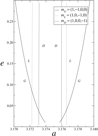
Figure 1: Unperturbed separatrices of guiding, layer and driving resonances in the plane $(a,e)$. (Nesvorný and Morbidelli, 1999)

Once the matrix of the transformation is defined, the new variables $\left(\mathbf{p,}\boldsymbol{\mathbf{\psi}}\right)$ can be rapidly obtained using the relations (7). In the new basis the arguments of the periodic terms change. The new vectors $\mathbf{\boldsymbol{\nu}}$ defined by $\mathbf{m}\cdot\mathbf{\boldsymbol{\theta}}=\boldsymbol{\mathbf{\nu}}\cdot\boldsymbol{\mathbf{\psi}}$ are shown in Table 1, in addition to the resonant vectors $\mathbf{m}$ and their respective coefficients.

The procedure of previous section was applied in the Nesvorný-Morbidelli model, and leads to the Hamiltonian (8) with $N=4$. The three perturbation coefficients $\beta_{G}$, $\beta_{L}$ and $\beta_{D}$ of the guiding, layer and driving resonances, respectively, are calculated at the resonant values $\mathbf{I}^{r}$, which satisfies (4). In the plane $N\Pi$ the resonant condition (4) leads to a curve satisfying to

$$\Pi^{r^{2}}+C_{1}\Pi^{r}+C_{2}=0,$$ (44)

where $C_{1}\left(N^{r}\right)$ and $C_{2}\left(N^{r}\right)$ are given in terms of $N^{r}$. Then, the solutions of (44) can be obtained analytically for a fixed value of $N^{r}$. However, in Nesvorný-Morbidelli model the coefficients $\tilde{\beta}_{\mathbf{m}}$’s are given as functions of the asteroid eccentricity (see Table 1). Therefore, we must use the definitions of Delaunay variables (30) to determinate $(a^{r},e^{r})$. The resonant eccentricity is determined through $e^{r}=\sqrt{1-\left(1+\Pi^{r}/N^{r}\right)^{2}},$ where $\left(N^{r},\Pi^{r}\right)$ satisfies (4). The resonant semi-major axis is determinate using $a^{r}=\left(N^{r}/2\right)^{2}.$

4 Numerical Experiments

In this section, we describe the numerical experiments done to investigate the diffusion across and along the stochastic layer of the three-body mean-motion resonance $\left(m_{J},m_{S},m\right)=(5,-2,-2)$ and its relations with the diffusion in semi-major axis and eccentricity. In these investigations the diffusion across will be described by the actions $(p_{1},p_{2})$ and the diffusion along by the actions $(p_{3},p_{4})$. In order to determine the time evolution of each action $\mathbf{p}$, we use the equations of motion obtained from Hamiltonian (8) with $N=4$. Then, for each value $p_{k}(t)$, we use the equations of transformation (7) to obtain the respective values of $N(t)$ and $\Pi(t)$ and the definition of the Delaunay actions in (30) to obtain $a(t)$ and $e(t)$.

Two main models were considered in the numerical experiments: (i) simplified (or two-resonance model) and (ii) complete (or three-resonance model). In the first one, only one term of the perturbation - the layer resonance - is considered. In the complete model, two terms are considered: the layer and one driving resonance. In both cases the guiding resonance is given by $\mathbf{m}_{G}=\left(1,-1,0,0\right)$.

Two different techniques were used to construct the solutions. In a first set of experiments, the equations of motion of the Hamiltonian (8) were numerically integrated using the Burlish-Stöer method, for times in the interval $10^{2}\leq t_{int}\leq 10^{8}$ years. The results of these simulations were sampled with an output time step of 10 years. The simulations were done for the eccentricities 0.05 and 0.25 with the initial conditions given on the separatrix of the guiding resonance $(p_{10}=2\sqrt{\left|M_{G}\beta_{G}^{r}\right|},p_{20}=0,p_{30}=0,p_{40}=0,\boldsymbol{\psi}=0)$. The main goal in these experiments was the study of the variation of the rate of diffusion across and along as a function of the total time of the simulations. Moreover, we investigate the correlations between the diffusion in the Chirikov actions $\mathbf{p}$ and the diffusion in semi-axis major and eccentricity.

In the other set of experiments, the simulations were done using an Hadjidemetriou-type sympletic mapping (Hadjidemetriou 1986, 1988, 1991, 1993; Ferraz-Mello 1997; Roig and Ferraz-Mello 1999, Lhotka 2009) defined by the canonical transformation $\left(\mathbf{p}^{n},\mathbf{\boldsymbol{\psi}}^{n}\right)\rightarrow\left(\mathbf{p}^{n+1},\mathbf{\boldsymbol{\psi}}^{n+1}\right),$ whose generating function is given by

$$S\left(\mathbf{p}^{n+1},\mathbf{\boldsymbol{\psi}}^{n}\right)=\sum\limits_{i=1}^{3}\psi_{i}^{n}p_{i}^{n+1}+\eta H\left(\mathbf{p}^{n+1},\mathbf{\boldsymbol{\psi}}^{n}\right),$$ (45)

where $\eta$ is the mapping step and the Hamiltonian is given by (8). The mapping equations are

$$p_{i}^{n+1}=p_{i}^{n}-\eta\frac{\partial H\left(\mathbf{p}^{n+1},\mathbf{\boldsymbol{\psi}}^{n}\right)}{\partial\psi_{i}^{n}}$$ (46)

$$\psi_{i}^{n+1}=\psi_{i}^{n}+\eta\frac{\partial H\left(\mathbf{p}^{n+1},\mathbf{\boldsymbol{\psi}}^{n}\right)}{\partial p_{i}^{n+1}}\qquad i=1,2,3.$$ (47)

The procedure to determinate the semi-major axis and eccentricity for each point $(p_{i}^{n+1},\psi_{i}^{n+1})$ of the trajectory is analogous to that discussed above. The goal of these experiments is to obtain the diffusion contour plots in the region of the 5,-2,-2 resonance in the plane $(a,e)$ (that plane is shown in Fig. 1) for the two models considered. In this case, the total time of integration used is the $10^{8}$ years with $\eta=10$ years. The initial conditions are defined by the knots of a grid in the plane $(a,e)$, on the rectangle $\left(3.17\leq a_{0}\leq 3.18\right)$U.A., $\left(0.01\leq e_{0}\leq 0.30\right)$. The initial condition of the state vector $\mathbf{p}_{0}$, for each point of the grid, was obtained using the transformation equations (7) and the definitions of Delaunay variables. The initial condition for the phases is $\psi_{k0}=0,k=1,\ldots 4$. The use of the Hadjidemetriou map was instrumental allowing the computation of the solutions starting on each point of the grid which, otherwise, would demand an excessively large amount of CPU-time. The comparison of results provided by the map with those obtained by integrating the Hamiltonian flow, do not show significant differences in the numerical computation of the diffusion coefficient (see below), at least for the two values of the eccentricity used (0.05 and 0.25).

Finally, we need a numerical procedure to estimate the diffusion coefficient of each element of the set $(p_{1},p_{2},p_{3},p_{4},a,e)$. In his investigations, Chirikov (1979, et al. 1979, 1985) used a particular method to determine the diffusion coefficient of the total energy $H$ of the system. After Chirikov (1979), this procedure allows the processes that are really stochastic to be separated from those associated to bounded oscillations of periodic nature. Chirikov’s procedure for experimental determination of the diffusion coefficient consist in dividing the total time of simulation $t_{int}$ in $N_{k}$ sub-intervals of length $\left(\Delta t\right)_{k}$ and the calculation of the mean value, $\bar{p}_{i}$, for every sub-interval. The contribution to the diffusion rate for a given pair $\bar{p}_{i_{m}}$, separated by interval of time $\left(m-\ell\right)\left(\Delta t\right)_{k}$, is given by $\left(\bar{p}_{i_{m}}-\bar{p}_{i_{\ell}}\right)^{2}/\left|m-\ell\right|\left(\Delta t\right)_{k}$. To obtain the rate of diffusion, the contributions of the considered pairs are averaged over all the combinations $m\neq\ell$. That is,

$$D_{i}^{k}=\frac{2}{N_{k}\left(N_{k}-1\right)}\sum_{m>\ell}\frac{\left(\bar{p}_{i_{m}}-\bar{p}_{i_{\ell}}\right)^{2}}{\left(\Delta t\right)_{k}\left(m-\ell\right)}.$$ (48)

The sub-intervals, used to estimate the mean values of quantities $\bar{p}_{i}$, were obtained with $k=10$ and the length $(\Delta t)_{10}=t_{int}/10$.

The same procedure was used to determine the diffusion of the semi-major axis, $D_{a}^{k}$, and of the eccentricity, $D_{e}^{k}$. We have also estimated the eccentricity variation in these experiments using a definition of diffusion rate of the random walking type (see for example Eqn. (24)):

$$\delta e\sim\sqrt{D_{e}^{k}t_{int}}.$$ (49)

5 Results and discussion

In this sections, we discuss the results obtained in the numerical experiments described above. In the discussion we will call action across to $(p_{1},p_{2})$, and across diffusion to $(D_{1},D_{2})$, where we suppressed the superscript $k$. In the same way we call action along to $(p_{3},p_{4})$ and along diffusion to $(D_{3},D_{4})$.

5.1 The role of number of the perturbing resonances in the diffusion

In his theory, Chirikov showed that the number of perturbing resonances is important for the dynamics of systems with many-dimensional Hamiltonians. The results, in this case, repeat what is know from the general theory of Hamiltonian systems. In a system with two degrees of freedom, the resonances may be isolated by KAM tori, but for $(N>3)$ the dimensionality may allows, in principle, a solution to visit the whole phase space when $t\to\infty$.

Several experiments, using the Burlish-Stöer integrator, were done see the way in which the number of perturbing resonances in the diffusion behavior. Figure 2 shows the results for the diffusion coefficients $D_{i},i=1,2,3,4$ in the simplified and complete models as function of total integration time for eccentricities equal to 0.05 and 0.25, . In the plots of Fig. 2, we see that the estimated diffusion increases in the low eccentricities up to a maximum reached for $10^{3}-10^{4}$ years. This behavior is explained by the fact that the solution needs to fill the stochastic domain in the direction across to it. After that maximum, in the simplified model the diffusion coefficients for all actions decrease continuously. This decrease indicates that the variation of the momenta in both directions, across and along the stochastic layer are bounded (as the total time increase, only the denominator of (48) grows making the result to decrease). As predicted by Chirikov’s theory of slow diffusion, the actions $p_{3}$ and $p_{4}$ along the resonance do not evolve, notwithstanding the absence of topological barriers for its evolution. Without a driving resonance, there is no long-period evolution of the solution along the stochastic domain. In our experiments, a very distinctive reduction in the diffusion is observed in the case $e=0.25$ after $t_{int}\sim 10^{7}$ years. This behavior is likely due to a sticking of the solution to some regular domain.

The behavior of the diffusion in the complete model is more complicated. In the experiment with $e=0.05$, the diffusion coefficients for the actions across the stochastic domain after $10^{8}$ years are smaller than for the actions along it. This difference reaches approximately four orders of magnitude in this case and is due, probably, to the limitation of the motion across the stochastic layer imposed by its width. For $e=0.25$ (right plot of Fig. 2), the diffusion coefficients in the two models present almost the same characteristics observed for $e=0.05$, except by the fact that, now, the diffusion in the actions along the stochastic layer, present a slow reduction with the integration time after $10^{4}$ years. This behavior is likely due to the absence of overlapping of resonance at high eccentricities, in contrast with the case of low eccentricities, where the three resonances overlap (see Fig. 1).

Figure 2: Diffusion coefficients of the actions associated with motion across and along the guiding resonance, in experiments over times from $10^{2}-10^{8}$ years for two different initial eccentricities.

5.2 Diffusion in semi-major axis and eccentricity in the complete model

The study of the previous section was completed with the computation of the diffusion coefficients for the orbital elements: semi-major axis and eccentricity in the complete model. Figure 3 presents the results. The results for the actions shown in this figure are the same shown in Fig. 2, but with a magnified scale. We see that, for large total times, there exist a correspondence between the diffusion coefficients of the actions across $(p_{1},p_{2})$ and of the semi-major axis, and between the diffusion coefficients of the actions along the resonance $(p_{3},p_{4})$ and of the eccentricity. This behavior can be understood observing the geometry of resonance $\left(5,-2,-2\right)$ shown in the Fig. 1. The separatrices of resonances are straight lines and the motion, along one of these separatrices, has constant semi-major axis and variable eccentricity. Following the discussion presented in Sect. 5.1, and the comparison done in the previous section for the simplified and completed models, we know that the drift along the separatrices only occurs if there is at least one driving resonance. Hence, the eccentricity diffusion is due to the driving resonance.

As a complement to the previous discussion, we note that the variations in semi-major axis occurs in the horizontal direction, the same direction of the actions $(p_{1},p_{2})$. The behavior of the diffusion in semi-major axis is similar to the diffusion of the actions across the resonance $(p_{1},p_{2})$ and is bounded by the width of the stochastic domain. A consequence of this fact is that the diffusion coefficient in the semi-major axis is smaller than that for the eccentricity (in the complete model, the diffusion along is not bounded).

The Fig. 4 shows the variation of the eccentricity calculated using initial conditions forming a grid in the plane $(a,e)$ (the same grid of Fig. 5) in $t_{int}=10^{8}$ years. The results for the simplified model are shown in Fig. 4(a). In this case, the larger variations in eccentricity occur for small values of the eccentricity. Two shallow maximums are formed, which are likely related with the eccentricity value at the intersection of the separatrices of the guiding and layer resonances (the only secondary resonance considered in the simplified model). The results for the complete model are shown in Fig. 4(b). In this case, the eccentricity variation reaches high values in the domain of low eccentricities - between $0.01$and $0.125$ - with a maximum for $<e>\sim 0.05$. This maximum is certainly a result of the overlapping of the resonances in low eccentricities, forcing the actions along the resonance.

In this model for mean eccentricities between 0.125 and 0.20 the variations are of the same order. The distributions observed in the Fig. 4(b) is in agreement with Nesvorný’s unpublished data for 45 numbered asteroids of the $(5,-2,-2)$ resonance (see the Table 2 in Nesvorný and Morbidelli 1998). The use of the models with only one perturbing resonance does not allow to get the distribution of the eccentricity variation observed in Fig. 4(b).

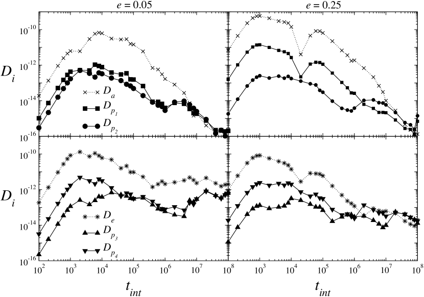
Figure 3: Diffusion Coefficient for actions across and along, semi-major axis and eccentricity in experiments, obtained for complete model, for times from $10^{2}$ up to $10^{8}$ years. Each point is one experiment with initial conditions upon the unperturbed separatrix of the guiding resonance.

Figure 4: Variation of the eccentricity versus mean eccentricity for (a) simplified model and (b) complete model on a net of points in the plane $(a,e)$.

5.3 The stochastic domain in the plane (a,e). Dependence on the initial conditions

The diffusion coefficients were calculated on a large set of initial conditions to assess the domain where the solutions present stochastic behavior. The analysis was done using simulations over $t_{int}\sim 10^{8}$ years, on the points of a grid of initial conditions in plane $(a,e)$. A Hadjidemetriou-type sympletic mapping was used instead of expensive numerical integration to allow a large number of simulations. Figure 5 shows the contour plots of the diffusion coefficients of $p_{4}$. It shows the stochastic domain of the guiding resonance (the light gray areas in Fig. 5). Note that the stochastic domain follows the geometry of the unperturbed separatrix of Fig. 1. Also note that the results for the complete model show a stochastic domain $(a,e)$ larger than that observed for the simplified model.

These differences are easily understood if we note the overlapping of the three resonances in the considered range of eccentricities. Figure 1 shows that the separatrices of the layer and driving resonances are, for almost all eccentricities, interior to the domain of the guiding resonance. At low eccentricities, however, the separatrices cross one another. Thus, in low eccentricities, one solution crossing the chaotic neighborhood of the separatrix of the guiding resonance, also cross the separatrices of the layer and driving resonances. The driving resonance acts pushing the actions along the guiding resonance. The magnitude of the push is determined by the phase $\varphi_{\mathbf{m}_{D}}$ and amplitude $\beta_{\mathbf{m}_{D}}$.

At variance with the complete model, the simplified model presents very low diffusion, in low eccentricities, as seen in Fig. 2. In this case, the absence of the driving resonance (only the guiding and layer are considered in the simplified model) implies in the absence of evolution along the guiding resonance.

A remarkable feature in both results is the formation of a wide region, in the central part of the domain of the guiding resonance, where the diffusion is negligible. The motion appears regular for initial conditions inside that region even when considering very long time spans. This result confirms what Nesvorný and Morbidelli (1999) observed in surface of sections for eccentricity $0.20$ using this same analytic model reduced to two degrees of freedom and two resonances. This is different from the situation observed in low eccentricities, where the separatrices of the resonances overlap.

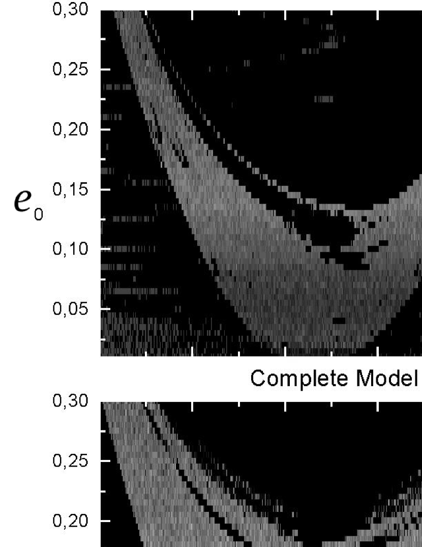
Figure 5: Diffusion coefficients for action along $p_{4}$ for initial conditions in the interval $3.17<a_{0}<3.18$ U.A. for semi-major axis and $0.01<e_{0}<0.30$ for eccentricity for both simplified and complete models. The results were obtained for total integration time equal to $10^{8}$ years.

6 Asymptotic behavior

Chirikov theory of slow diffusion was constructed to study the diffusion under the action of an arbitrarily weak perturbations, and the diffusion coefficient was computed there using the asymptotic estimate of Melnikov’s Integral. The asymptotic behavior of the three-body resonance model of Nesvorný and Morbidelli was studied using the same technique devised by Chirikov. Figure 6 shows the variation of the diffusion coefficients along the resonance, for two different initial eccentricities (0.05 and 0.2), as functions of the parameter $\lambda_{\mathbf{m}_{D}}=\omega_{\mathbf{m}_{D}}/\Omega_{G}$ appearing as argument of the Melnikov integrals in Sect. 2.3 in the case the driving resonance $\mathbf{m}=\left(1,0,0,-1\right)$. Small values of $\lambda_{\mathbf{m}_{D}}$ are obtained decreasing the intensity of the guiding and perturbing resonances.

The Hadjidemetriou-like mapping was used to allow us to compute the solutions over $10^{10}$ years for a great deal of different conditions. The diffusion coefficient was calculated for initial conditions over the separatrix of the guiding resonance. A background value $D_{b}$, to be used as reference, was also obtained with initial conditions in the central part of the guiding resonance, far from the separatrices. For small values of the perturbation, the motion in the central part of the resonance domain is regular and the background diffusion appear as smaller than the diffusion shown by solution starting on the separatrices. For high values of the perturbation intensity, the motion is chaotic over the whole domain and the diffusion coefficients in the central part are not different form those of solutions starting on the separatrices.

Figure 6 shows the diffusion coefficient $D_{3}$ for $e=0.2$ and for the low eccentricity case $e=0.05$. The figures for the coefficient $D_{4}$ are not shown since they are almost identical to those shown for $D_{3}$. Figure 6 shows the 3 different possibilities.

1. The first section of the figures, corresponding roughly to $\lambda_{\mathbf{m}_{D}}\lesssim 2$, is characterized by complete chaos. For the smallest $\lambda_{\mathbf{m}_{D}}$, one sees the same phenomenon discussed in Sect. 5.1: the background diffusion appear small for some shorter runs because they do not cover the time necessary to allow the solution to fill the chaotic layer; but when time span grows, the diffusion values increase as expected. In this section, in general the diffusion coefficients for solutions starting in the central part or on the separatrices are equal showing that the whole resonance domain is chaotic. A few exceptions appear, as shown in Fig. 6(b). In addition we may see in this figure, for $\lambda_{\mathbf{m}_{D}}\sim 1$, a sudden decrease of the background diffusion indicating that the corresponding solution stuck to some regularity island during its evolution. However this sticking is not permanent and the background diffusion grows when longer time spans are considered. The background values are shown in Fig. 6(a) only for the time span $10^{10}$ years to allow a better comparison of the numerical results with the dashed lines representing results from Chirikov’s model,

2. For $\lambda_{\mathbf{m}_{D}}\sim 2$, the background diffusion shows a discontinuity which, for the longest runs, reaches up to 14 orders of magnitude. This means that the center of the resonance domain becomes regular and the stochasticity remains confined to layers around the separatrix. This is the domain where Chirikov’s slow diffusion theories are valid and where the results may be compared to the theoretical results obtained in Sect. 2.4. The integration time is a crucial factor in the detection of the slow diffusion. For instance, one may see that for simulations over only $10^{5}$ years, the diffusion near separatrix is equal to the background diffusion for values of $\lambda_{\mathbf{m}_{D}}$ close to 1, while for simulations over $10^{10}$ years, the equality is reached only for $\lambda_{\mathbf{m}_{D}}=9$.

3. In the last section of the Figs. 6 the solutions starting close to the separatrices show a diffusion equal to the background diffusion. The interpretations is that the stochastic layer is this case is so thin that the used initial conditions are no longer within them. (For that sake, the locus of the separatrices should be computed with very large precision. See e.g. Froeschlé et al. 2006). One striking feature in this section is that an increase in the time span by a factor 10 means a decrease in the background diffusion by a factor $10^{3}$. This is a clue for the fact that the solutions are dominated by periodic terms. Indeed, if we consider one periodic term with amplitude proportional to $\epsilon$ and frequency $\omega$, its contribution to the average momentum in an interval $\left[a,b\right]$ is proportional to

   $$\frac{1}{\Delta t}\intop_{a}^{b}\epsilon\mbox{cos}\omega tdt$$

   where $\Delta t=b-a$. This integral is elementary and the integration of the result over all frequencies below a upper limit $\omega_{\text{lim}}$, gives

   $$\frac{\epsilon}{\Delta t}\left[\mbox{si}\left(b\omega_{\text{lim}}\right)-\mbox{si}\left(a\omega_{\text{lim}}\right)\right]$$

   where si is the sine-integral function. The diffusion coefficients are given by the square of the average variation of the momentum divided by the total time (see Eqn. 24) and then $D\sim\Delta t^{-3}$. We also have $D\varpropto\epsilon^{2}\sim\Omega_{G}^{-2}\sim\lambda_{D}^{-4}$. The inclination -4 of the straight lines in the log-log plots can be easily checked.

The diffusion of the solutions in the neighborhood of the separatrix may be determined from Eqn. 27. This equation involves the intensity of the perturbation (related to $\lambda_{\mathbf{m}_{D}}$) and two unknown parameters: the factor of reduction $R_{\mathbf{m}_{D}}$ and the factor of odd perturbations $R_{T}$. The factor of reduction corresponds to Chirikov’s hypothesis of reduced stochasticity (due to holes, the solution does not fill the strip around the separatrix); the other factor comes from the fact that the perturbation is not even and thus the values of the diffusion coefficient are not the same for solutions in both separatrices (the solution may remain circulating near one of the separatrices at time different of the time it remain near the other).

The results obtained with Chirikov are shown in Figs. 6 by dashed lines. In Figs. 6(a) tree different solutions are shown (calculated with the reduction factors indicated in the figure). The better agreement is obtained with $R_{\mathbf{m}_{D}}=0.25$. The two values used for $R_{T}$ (0.6 and 0.9) give almost the same result, showing that the motion near deviation for the weakest perturbation (larger $\lambda_{\mathbf{m}_{D}}$). In the other two figures, only the two solutions with $R_{\mathbf{m}_{D}}=0.25$ are shown.

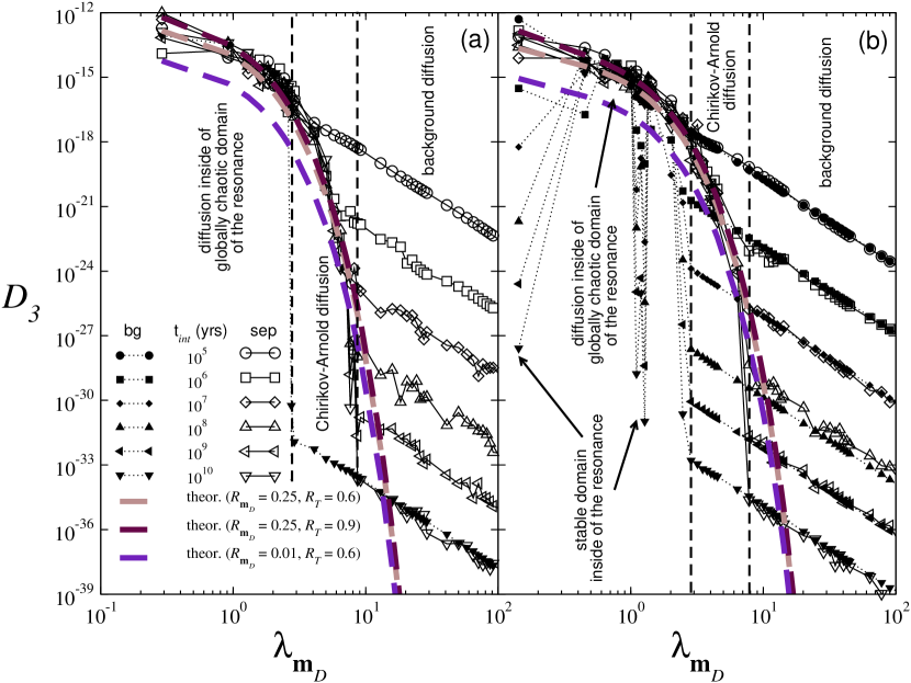
Figure 6: Asymptotic behavior of the diffusion coefficient $D_{3}$ for initial conditions over the separatrix and on the central part of the guiding resonance for (a) $e=0.05$ and (b) $e=0.20$. The dashed lines show the behavior predicted with Chirikov’s theory.

7 Conclusion

Chirikov’s theories provide heuristic tools to understand the diffusion observed in both eccentricity and semi-major axis of asteroids inside the $\left(5,-2,-2\right)$ resonance. The multi-dimensional Hamiltonians of the three-body (three orbit) mean-motion resonances may be studied with the theories developed by Chirikov and collaborators, mainly because of the particular geometry of those resonances in the plane $\left(a,e\right)$. The results obtained in this paper for the $\left(5,-2,-2\right)$ three-body mean-motion resonance confirms the role of the resonances in the raising of diffusion across and along the main resonance as foreseen in Chirikov’s theories.

The diffusion calculations presented in this paper show that diffusion in semi-major axis is related with the diffusion in the across actions $(p_{1},p_{2})$ while the diffusion in eccentricity is related with the diffusion in the along actions $(p_{3},p_{4})$. The diffusion coefficient for the semi-major axis tends to small values showing that the variation of the semi-major axis remains small. It indicates the existence of barriers on both sides of the stochastic layer limiting the motion across the resonance.

The comparison between simplified and complete model results shown that the diffusion in eccentricity is presumably due to the presence of at least one resonance driving the motion along the guiding resonance. This behavior is similar to the expected behavior of the Arnold diffusion, but, differently of it, the diffusion here is well apparent and the diffusion coefficients remain high. For this reason it was sometimes called Fast Arnold Diffusion (Chirikov and Vecheslavov 1989, 1993).

The structure of the $\left(5,-2,-2\right)$ resonance is formed by several overlapping resonances, particularly at low eccentricities. Thus, diffusion across $\left(5,-2,-2\right)$ resonance may be no longer limited to the thin chaotic layers (stochastic layers), but it fills the whole resonance zone. The diffusion along the resonance could be due to a multiplet. In this scenario, we have a random motion across the resonance, due to the overlap of several resonances belonging to a multiplet, and another, likely due to weaker resonances, which drive the diffusion along the guiding resonance. Arnold diffusion might occur inside the stochastic layer formed around the separatrix of the guiding resonance under the action of sufficiently weak perturbations. At variance, thick layer diffusion can appear for perturbation parameters in a broad interval. Although this mechanism show a similar exponential dependence of diffusion rate as a function of some system parameters, the mean rate of thick layer diffusion is generally larger than any theoretical estimation of Arnold diffusion. Therefore, it seems that for the real problem would be more appropriate to call the diffusion with another name - asymptotic diffusion of Chirikov-Arnold - due to the fact that this keeps some features of the Arnold diffusion, but late very well characterized by Chirikov like some distinct.

As we mentioned before, we believe that the connection between rigorous investigations concerning strictly Arnold diffusion and that observed in real physical systems like this, is still an open subject. As Lochak (1999) pointed out, the global instability properties of near–integrable Hamiltonian systems are far from well–understood. It could almost be said that little progress has been made after pioneering work Arnold, and new ideas are definitely called for.

Finally, the good results showed that the Chirikov slow diffusion theory can be used in broader investigations considering more resonances for $\left(5,-2,-2\right)$, as well applied for the others three-body (three orbit) mean motion resonances and also can include the inclination of the asteroid orbit.

Appendix A Estimate of total variation of the momenta $p_{k}$’s

To estimate the integral in (20 we use the approach done by Chirikov (1979). In fact, the unperturbed separatrix is defined by

$$\psi_{1}^{sx}\left(t\right)=4\textrm{arctan}\left(e^{\pm\Omega_{G}\left(t-t^{0}\right)}\right),$$ (50)

$$p_{1}^{sx}=\pm 2\left|M_{G}\right|\Omega_{G}\textrm{sin}\frac{\psi_{1}^{sx}}{2},$$ (51)

where

$$\Omega_{G}=\sqrt{\epsilon\left|\frac{V_{G}}{M_{G}}\right|}$$ (52)

is the proper frequency of the pendulum Hamiltonian $H_{1}$. The double sign indicates the two separatrix branches: The positive sign correspond to the upper separatrix $\left(0\leq\psi_{1}^{sx}<2\pi\right)$, and the negative corresponds to the lower separatrix $\left(-2\pi\leq\psi_{1}^{sx}<0\right)$. The stable equilibrium points lie at $\psi_{1}=\pm\pi$, respectively. (This non usual separation of the intervals where the two branches are considered allows $\psi_{1}$ and $p_{1}$ to have the same signal in each separatrix and simplifies the next calculations. For the usual presentation, the reader is referred to the study of the motions near the separatrix of pendulum in the Appendix B of Ferraz-Mello, 2007.)

We introduce a time variable change $\tau=\Omega_{G}\left(t-t^{0}\right)$, with $\psi_{1}^{sx}\left(t^{0}\right)=\psi_{1}^{0}=\pm\pi$. Then, to $\psi_{1}^{s}>0$ (lower separatrix), we have

$$\sin\varphi_{\mathbf{m}}^{sx}\left(t\right)=\sin\left(\xi_{\mathbf{m}}\psi_{1}^{sx}\left(\tau\right)+\lambda_{\mathbf{m}}\tau+\varphi_{\mathbf{m}}^{0}\right),$$ (53)

where $\varphi_{\mathbf{m}}^{0}=\xi_{\mathbf{m}}\psi_{1}^{0}+\omega_{\mathbf{m}}t^{0}+\beta_{\mathbf{m}}$, with $\psi_{1}^{0}=\pi$, and

$$\lambda_{\mathbf{m}}=\frac{\omega_{\mathbf{m}}}{\Omega_{G}}.$$ (54)

Or, after expansion of the right-hand side,

$$\sin\varphi_{\mathbf{m}}^{sx}\left(t\right)=\sin\left(\xi_{\mathbf{m}}\psi_{1}^{sx}\left(\tau\right)+\lambda_{\mathbf{m}}\tau\right)\cos\varphi_{\mathbf{m}}^{0}+\cos\left(\xi_{\mathbf{m}}\psi_{1}^{sx}\left(\tau\right)+\lambda_{\mathbf{m}}\tau\right)\sin\varphi_{\mathbf{m}}^{0}.$$ (55)

When (55) is substituted into (20), the first term does not give contribution since, by symmetry,

$$\int_{{}_{-\infty}}^{{}^{+\infty}}\sin\left[\xi_{\mathbf{m}}\psi_{1}^{sx}\left(\tau\right)+\lambda_{\mathbf{m}}\tau\right]d\tau=0.$$ (56)

The contribution of the second term of (55) is determined by the relative signs of $\xi_{\mathbf{m}}$ and $\lambda_{\mathbf{m}}$. Using the absolute values to $\xi_{\mathbf{m}}$ and $\lambda_{\mathbf{m}}$, we can introduce the Melnikov integral in the form

$$\int_{{}_{-\infty}}^{{}^{+\infty}}\cos\left(\left|\xi_{\mathbf{m}}\right|\psi_{1}^{sx}\left(\tau\right)\pm\left|\lambda_{\mathbf{m}}\right|\tau\right)d\tau=\frac{1}{\Omega_{G}}A_{2\left|\xi_{\mathbf{m}}\right|}\left(\mp\left|\lambda_{\mathbf{m}}\right|\right),$$ (57)

where $A_{2\left|\xi_{\mathbf{m}}\right|}$ is the Melnikov integral with argument $\pm\left|\lambda_{\mathbf{m}}\right|$. Then, the integral in (20) is

$$\int_{{}_{-\infty}}^{{}^{+\infty}}\sin\varphi_{\mathbf{m}}^{sx}\left(t\right)dt=\frac{1}{\Omega_{G}}\textrm{sin$\varphi_{\mathbf{m}}^{0}$}A_{2\left|\xi_{\mathbf{m}}\right|}\left(\mp\left|\lambda_{\mathbf{m}}\right|\right).$$ (58)

In the other branch of the separatrix, $\psi_{1}^{sx}$ has the signal changed, but the particular symmetry of this equation makes it invariant to the sign change of $\psi_{1}^{sx}$ and, thus, one obtains the same result (58). Indeed, if $\psi_{1}^{sx}<0$ the parity of cosine makes the integral (57) to be

$$\int_{{}_{-\infty}}^{{}^{+\infty}}\cos\left(\left|\xi_{\mathbf{m}}\right|\left|\psi_{1}^{sx}\left(\tau\right)\right|\mp\left|\lambda_{\mathbf{m}}\right|\tau\right)d\tau=\frac{1}{\Omega_{G}}A_{2\left|\xi_{\mathbf{m}}\right|}\left(\pm\left|\lambda_{\mathbf{m}}\right|\right),$$ (59)

where we used $\psi_{1}^{sx}\left(\tau\right)=-\left|\psi_{1}^{sx}\left(\tau\right)\right|$. Then, the variations in the actions $p_{k}$ can be obtained introducing the result (59) into (20):

$$\Delta p_{k}\left(t\right)\approx\frac{\epsilon}{\Omega_{G}}\sum\limits_{\mathbf{m\neq\mathbf{m}}_{G}}\nu_{k}\left(\mathbf{m}\right)V_{\mathbf{m}}^{r}\textrm{sin$\varphi_{\mathbf{m}}^{0}$}\left[A_{2\left|\xi_{\mathbf{m}}\right|}\left(\left|\lambda_{\mathbf{m}}\right|\right)+A_{2\left|\xi_{\mathbf{m}}\right|}\left(-\left|\lambda_{\mathbf{m}}\right|\right)\right].$$ (60)

Chirikov (1979) estimated the diffusion using the result of the last equation. In order to simplify the theoretical estimate of the diffusion, Chirikov considered only even perturbing resonances and neglected the contribution of the perturbation with negative argument under the condition $\left|\lambda_{\mathbf{m}}\right|\gg 1$.

In the case of the three-body mean-motion resonance model, the perturbation are non even and it is not possible to neglect the contribution of perturbations for which $\left|\lambda_{\mathbf{m}}\right|$ is small. Then, each perturbation contributes differently when the motion lies close to a separatrix where $\lambda_{\mathbf{m}}>0$ or $\lambda_{\mathbf{m}}<0$. Moreover, the odd perturbations in the Nesvorný-Morbidelli model makes necessary to take into account that the times of permanence of the motion near each separatrix are not equal. This is done by considering that the solution lies only a fraction of total time near the separatrix with $\lambda_{\mathbf{m}}>0$. To take into account this asymmetry we introduce the factor $R_{T}$

$$R_{T}=\frac{T_{\lambda}}{T},$$ (61)

where $T_{\lambda}$ is the time that the solution stay in the neighborhood of separatrix with $\lambda_{\mathbf{m}}>0$ and $T$ is the total time. Then, the Eqn. (60) is rewritten as

$$\Delta p_{k}\approx\frac{\epsilon}{\Omega_{G}}\sum\limits_{\mathbf{m}\neq\mathbf{m}_{G}}\nu_{k}\left(\mathbf{m}\right)Q_{\mathbf{m}}\sin\varphi_{\mathbf{m}}^{0},$$ (62)

with

$$Q_{\mathbf{m}}=V_{\mathbf{m}}^{r}\left[R_{T}A_{2\left|\xi_{\mathbf{m}}\right|}\left(\left|\lambda_{\mathbf{m}}\right|\right)+\left(1-R_{T}\right)A_{2\left|\xi_{\mathbf{m}}\right|}\left(-\left|\lambda_{\mathbf{m}}\right|\right)\right].$$ (63)

Equation (62) is valid for non-even perturbation and for small $\lambda_{\mathbf{m}}$. In order to obtain estimation of (62) in terms of ordinary functions we must know the values of $\left|\lambda_{\mathbf{m}}\right|$ and $\left|\xi_{\mathbf{m}}\right|$. In general, the relations to $A_{2\left|\xi_{\mathbf{m}}\right|}$ depend on the exponential term with argument $\left|\lambda_{\mathbf{m}}\right|$ (see Appendix A in Chirikov 1979).

References

- (1) Benettin, G., and Gallavotti, G.: Stability of Motions near Resonances in Quasi-Integrable Hamiltonian Systems, J. Stat. Phys. 44, 293-338 (1986).
- (2) Berry, M.: in Topics in nonlinear dynamics: A tribute to Sir Edward Bullard New York, American Institute of Physics, 1978, p. 16-120 (1978)
- (3) Chirikov, B.V.: A universal instability of many-dimensional oscillator system. Phys. Rep. 52, 263-379 (1979)
- (4) Chirikov, B.V., Ford, J. and Vivaldi, F.: Some numerical studies of Arnold diffusion in simple model. In: M. Month. and J.C. Herrera (eds) A.I.P. Conf. Proc.: Nonlinear Dynamics and the Beam-Beam Interaction, N 57, pp. 323-340 (1979)
- (5) Chirikov, B.V., Lieberman, M.A., Shepelyansky, D.L. and Vivaldi, F.M.: 1985, A theory of modulational diffusion, Physica 14D, 289-304.
- (6) Chirikov, B.V. and Vecheslavov, V.V.: How fast is the Arnold diffusion? Preprint INP 89-72, Novosibirsk (1989)
- (7) Chirikov, B.V. and Vecheslavov, V.V.: Theory of fast Arnold diffusion in many frequency system. J. Stat. Phys. 71, 243 (1993)
- (8) Cincotta, P.M.: Arnold diffusion: an overview through dynamical astronomy. New Astronomy Reviews 46, 13-39 (2002)
- (9) Cincotta, P.M. and Giordano, C.M: Topics on diffusion in phase space of multidimensional Hamiltonian systmes. In: New Nonlinear Phenomena Research, Nova Science Publishers, Inc., pp. 319-336, (2008)
- (10) Dermott, S. F.and Murray, C. D.: Nature of the Kirkwood gaps in the asteroid belt. Nat.301, 201-205 (1983)
- (11) Ferraz-Mello, S., Nesvorný, D.and Michtchenko, T. A. On the Lack of Asteroids in the Hecuba Gap. Celest. Mech. Dynam. Astron. 69, 171-185 (1997)
- (12) Ferraz-Mello, S.: A sympletic mapping approach to the study of the stochasticity of asteroidal resonances. Cel. Mech. Dyn. Astron. 65, 421-437 (1997)
- (13) Ferraz-Mello, S.: Canonical Perturbation Theories - Degenerate Systems and Resonance. Springer, New York (2007)
- (14) Froeschlé, C., Lega, E. and Guzzo, M.: Analysis of the chaotic behavior of orbits diffusing along the Arnold Web. Celest. Mech. Dynam. Astron. 95, 141-153 (2006)
- (15) Giordano, C. M. and Cincotta, P.M.: Chaotic diffusion of orbits in systems with divided phase space. A&A. 423, 745-753 (2004)
- (16) Guzzo, M., Lega, E. and Froeschlé, C.: A Numerical Study of Arnold Diffusion in a Priori Unstable Systems. Comm. in Math. Phys., 290, 557-576 (2009a)
- (17) Guzzo, M., Lega, E. and Froeschlé, C.: A numerical study of the topology of normally hyperbolic invariant manifolds supporting Arnold diffusion in quasi-integrable systems. PhysD, 238, 1797-1807 (2009b)
- (18) Hadjidemetriou, J. D. and Ichtiaroglou, S.:A qualitative study of the Kirkwood gaps in the asteroids.A&A. 131, 20-32 (1984)
- (19) Hadjidemetriou, J.D.: A hyperbolic twist mapping model for the study of asteroid orbits near the 3/1 resonance. J. Appl. Math. Phys. 37, 776-796 (1986)
- (20) Hadjidemetriou, J.D.: Algebric mappings near the resonance with an application to asteroid motions. In: A.E. Roy (ed) Long Term Dynamical Behavior of Natural Artificial and N-body Systems. Kluver Academic Publishers, 257-276 (1988)
- (21) Hadjidemetriou, J.D.: Mapping models for Hamiltonian system with application to resonant asteroidal motion. In: A.E. Roy (ed) Predictability, Stability and Chaos in N-body Dynamical Systems, Plenum Press, 157-175 (1991)
- (22) Hadjidemetriou, J.D.: Asteroid motion near the 3/1 resonance. Cel. Mech. Dyn. Astron. 56, 563-599 (1993)
- (23) Knežević, Z.: Veritas family age revisited. In: IAU Coloquium 173: Evolution and sources regions of asteroids and comets, pp 153-158 (1999)
- (24) Knežević, Z., Tsiganis, K. and Varvoglis, H.: The dynamical portrait of the Veritas family region. In: Proceedings of Asteroids, Comets, Meteors International Conference, Noordwijk, Netherlands: ESA Publications Division, pp. 335-338 (2002)
- (25) Knežević, Z.: Chaotic diffusion in the Veritas family region. In: Proceedings of the XIII National Conference of Yugoslav Astronomers, Publications of the Astronomical Observatory of Belgrade 75, pp. 251-254 (2003)
- (26) Knežević, Z.: New Frontiers in Main Belt Asteroid Dynamics. In: Bulletin of the American Astronomical Society, 36, p. 856 (2004)
- (27) Knežević, Z., Tsiganis, K. and Varvoglis, H.: Age of the Veritas asteroid family from two independent estimates. Astronomical Observatory of Belgrade, 80, p. 161-166 (2004)
- (28) Knežević, Z.: Dynamical Methods to Estimate the Age of Asteroid Families. (2007)
- (29) Lega, E. Guzzo, M. and Froeschlé, C.: Measure of the exponential splitting of the homoclinic tangle in four-dimensional symplectic mappings. Celest. Mech. Dyn. Astron. 104, 191-204 (2009)
- (30) Lochak, P.: Arnold diffusion: A compendium of remarks and question. In: C. Simó (ed) NATO ASI: Hamiltonian system with Three or More Degrees of Freedom, pp-168, Kluver, Dordrecht (1999)
- (31) Lhotka, C.: Dynamic expansion points: an extension to Hadjidemetriou’s mapping methods. Celest. Mech. Dyn. Astron. 104, 175-189 (2009)
- (32) Lichtenberg, A.J. and Lieberman, M.A.: Regular and Stochastic Motion. Springer-Verlag, New York, vol. 38 (1983)
- (33) Milani, A. and Nobili, A. M.: An example of stable chaos in the solar system. Nature 357, 569-571 (1992)
- (34) Milani, A.: 1993, The trojan asteroid belt: Proper elements, stability, chaos and families. Celest. Mech. Dyn. Astron. 57, 59-94 (1993)
- (35) Milani, A.; and Farinella, P.: The age of the Veritas asteroid family deduced by chaotic chronology. Nature 370, 40-42 (1994)
- (36) Milani, A.; Nobili, A. M.; Knežević, Z.: Stable chaos in asteroid belt. Icarus 125, 13-31 (1997)
- (37) Morbidelli, A. and Froeschlé, C.: On the relationship between Lyapunov times and macroscopic instability times. Celest. Mech. Dyn. Astron. 63, 227- 239 (1996)
- (38) Nesvorný, D. and Morbidelli, A.: Three-body mean-motion resonances and the chaotic structure of the asteroid belt. Astron. J. 116, 3029-3037 (1998)
- (39) Nesvorný, D. and Morbidelli, A.: An analytic model of three-body mean-motion resonances. Celest. Mech. Dyn. Astron. 71, 243-271 (1999)
- (40) Novaković, B.; Tsiganis, K.; Knežević, Z.: Chaotic transport and chronology of complex asteroid families. (2009)
- (41) Roig, F. and Ferraz-Mello.: A sympletic mapping approach of the dynamics of the Hecuba gap. Planetary and Space Science 47, 653-664 (1999)
- (42) Sun, Y and Zhou, L.: Stickiness in three-dimensional volume preserving mappings. Celest. Mech. Dyn. Astron.103, 119-131 (2009)
- (43) Tsiganis, K., Varvoglis, H. and Hadjidemetriou, J. D. Stable Chaos in High-Order Jovian Resonances. Icarus 155, 454-474 (2002a)
- (44) Tsiganis, K., Varvoglis, H. and Hadjidemetriou, J. D. Stable Chaos versus Kirkwood Gaps in the Asteroid Belt: A Comparative Study of Mean Motion Resonances. Icarus 159, 284-299 (2002b)
- (45) Varvoglis, H: Diffusion in the asteroid belt. In: IAU Coloquium 197: Dynamics of Populations of Planetary Systems, pp 157-170 (2004)
- (46) Tsiganis, K., Knežević, Z. and Varvoglis, H.: Reconstructing the orbital history of the Veritas family. Icarus 186, 484-497 (2007).
- (47) Wisdom, J.:The origin of the Kirkwood gaps - A mapping for asteroidal motion near the 3/1 commensurability. A.J. 87, 577-593 (1982)