Perpetual Cancellable American Call Option

Abstract.

This paper examines the valuation of a generalized American-style option known as a Game-style call option in an infinite time horizon setting. The specifications of this contract allow the writer to terminate the call option at any point in time for a fixed penalty amount paid directly to the holder. Valuation of a perpetual Game-style put option was addressed by Kyprianou (2004) in a Black-Scholes setting on a non-dividend paying asset. Here, we undertake a similar analysis for the perpetual call option in the presence of dividends and find qualitatively different explicit representations for the value function depending on the relationship between the interest rate and dividend yield. Specifically, we find that the value function is not convex when $r>d$. Numerical results show the impact this phenomenon has upon the vega of the option.

1. Introduction

In current times, it is not hard to imagine a financial system burdened by illiquidity over a large cross section of total market activity. Under such circumstances, trading in the market might cease to be an option even for large financial firms interested in hedging their short contracts. Indeed, cancelling or recalling such contracts might be one of the few ways to effectively mitigate undesirable positions in turbulent times. As such, derivative securities which include callback provisions or cancellable features represent attractive instruments to writers of these contracts. The following discussion addresses the valuation of a common American-style claim with the aforementioned termination specification built into the contract.
Kifer (2000) was the first to broach the problem of valuation for American-style options with a cancellation feature available to the short side of the contract. In that article, Kifer applied the continuous time game theoretic results of Lepeltier and Maingueneau (1984) to these generalized American options and found the fair price was equal to the value of a Dynkin game (see e.g. Dynkin (1969), Neveu (1975)) between the long and the short sides of the contract. The close relationship between these options and Dynkin games fostered a renewed interest in such games and subsequently brought forth general existence and characterization results about the value of a Dynkin game (see e.g. Alvarez (2008), Ekström (2006), Ekström and Villeneuve (2006), Ekström and Peskir (2008), Peskir (2008)). With respect to game options, Kuhn, Kyprianou, and van Schaik (2007) recently extended valuation results in a complete market framework to include more general payoffs than those considered in Kifer (2000). Recent results in an incomplete market setting include Kuhn (2004), and Hamadène and Zhang (2008).
Since game-type derivatives are generalized American-style options, explicit solutions are rare in many settings. However, Kyprianou (2004) explicitly solved, under the Black-Scholes framework, the valuation problem associated to a particular game-type derivative known as the perpetual Israeli $\delta$-penalty put option. This analysis was limited to a put option on a non-dividend paying asset following geometric brownian motion. Within this framework, Kyprianou found that the strike price was the only asset value for which optimal contract termination would occur. This result for the put option is intuitive and, perhaps, suggests similar behavior for its call option counterpart. Following that article, Kuhn and Kyprianou (2007) addressed the finite expiry put option valuation problem and found its explicit representation as a compound exotic option. In the following discussion, we consider the valuation problem of a perpetual game call option on a dividend paying asset. Recently, Kunita and Seko (2004) considered the finite expiry version of this contract. Here, we utilize some of the same arguments while attempting to explicitly solve the valuation problem. In doing so, we find significant qualitative differences with Kunita and Seko’s finite expiry analysis and important distinctions from the work done by Kyprianou (2004) on an infinite expiry game put option with a non-dividend paying asset. Most recently, Alvarez (2009) explicitly characterized both the value and the optimal exercise policy of a minimum guaranteed payment game option when the underlying asset price follows a general linear, time homogeneous diffusion. The payoff structure Alvarez (2009) considered is, indeed, very similar to a game call option since the payoff of the former upon exercise by the holder is $\max(X-K_{1},0)+K_{2}$ where $K_{1}=K_{2}>0$. Our analysis here is distinct from Alvarez (2009) since a regular call option payoff assumes $K_{1}\geq 0$ and $K_{2}=0$. We find that this slight parameter difference significantly changes the solution to the optimal stopping problem even in the typical case when the underlying dynamics follow geometric brownian motion.

The forthcoming discussion is organized as follows. Section 2 describes the economic setting and presents a few foundational valuation results. Section 3 addresses the valuation problem when $r\leq d$. Section 4 examines valuation when $r>d$. Section 5 presents results from a numerical approximation of the optimal exercise and cancellation boundaries. Section 6 concludes the valuation discussion. Section 7 elaborates on a few claims from prior sections.

2. Setup

The economic setting is the standard financial market with constant coefficients. We assume the underlying asset process follows the geometric Brownian Motion process whose price satisfies

(2.1) $$\begin{split}\mathrm{d}X_{t}=(r-d)X_{t}\mathrm{d}t+\sigma X_{t}\mathrm{d}W_{t}\end{split}$$

where $r$ is the risk-free rate of interest assumed to be strictly positive, $d$ is the dividend rate on the underlying asset assumed to be non-negative, and $\sigma$ is the volatility of the asset’s return assumed to be strictly positive. The dynamics in (2.1) describe the risk-neutralized evolution of the underlying asset process. The process $W$ is a Brownian motion under the risk-neutral measure $\mathbb{P}$.
Let $V^{*}(X_{t})$ denote the value at $t$ of a perpetual call option with a cancellation feature available to the short side of the contract with penalty $\delta$. That is, the payoff to the holder upon cancellation when $X_{t}=x$ is $(x-K)^{+}+\delta$. We will refer to this contract as a perpetual $\delta$-penalty call option or simply a $\delta$-penalty call option. If the holder exercises with strategy $\sigma$ and the writer cancels with strategy $\tau$, then payoff to the holder of the contract is $Z_{\sigma,\tau}$ where

(2.2) $$Z_{s,t}:=(X_{s}-K)^{+}1_{\{s\leq t\}}+((X_{t}-K)^{+}+\delta)1_{\{t<s\}}$$

Please note that we denote both the volatility of the geometric brownian motion and the holder’s exercise stopping time by $\sigma$. In the sequel, it will be clear by the context as to which quantity $\sigma$ references. Standard results (see e.g. Kyprianou (2004)) can be invoked to establish that the value of the $\delta$-penalty call option is

(2.3) $$\begin{split}V^{*}(x)&=\inf_{\tau\in\mathcal{S}_{0,\infty}}\sup_{\sigma\in\mathcal{S}_{0,\infty}}\mathbb{E}[e^{-r(\sigma\wedge\tau)}\{((xN_{\tau}-K)^{+}+\delta)1_{\{\tau<\sigma\}}+(xN_{\sigma}-K)^{+}1_{\{\sigma\leq\tau\}}\}]\\ &=\sup_{\sigma\in\mathcal{S}_{0,\infty}}\inf_{\tau\in\mathcal{S}_{0,\infty}}\mathbb{E}[e^{-r(\sigma\wedge\tau)}\{((xN_{\tau}-K)^{+}+\delta)1_{\{\tau<\sigma\}}+(xN_{\sigma}-K)^{+}1_{\{\sigma\leq\tau\}}\}]\\ \end{split}$$

where

(2.4) $$N_{t}:=\exp{\{(r-d-\frac{\sigma^{2}}{2})t+\sigma W_{t}\}}$$

with optimal exercise strategies for the holder and writer respectively equal to

(2.5) $$\begin{split}\sigma^{*}&=\inf{\{t\in[0,\infty):V^{*}_{t}=(X_{t}-K)^{+}\}}\\ \tau^{*}&=\inf{\{t\in[0,\infty):V^{*}_{t}=(X_{t}-K)^{+}+\delta\}}\end{split}$$

where $\inf{\{\emptyset\}}=\infty$, by convention. We shall adopt this convention throughout the entire paper. Note $\mathcal{S}_{0,\infty}$ denotes the set of all stopping times of the Brownian filtration, and $\mathbb{E}$ is the expectation under the risk-neutral measure $\mathbb{P}$. In addition, let $\mathbb{E}_{x}$ denote the expectation under $\mathbb{P}$ such that $X_{0}=x$.
We begin our discussion with a regularity result for the value function of the $\delta$-penalty call option.

Proposition 2.1.

The value function is non-decreasing in $x$ and is Lipschitz continuous with Lipschitz constant $1$.

Proof.

Recall,

$$V^{*}(x)=\inf_{\tau\in\mathcal{S}_{0,\infty}}\sup_{\sigma\in\mathcal{S}_{0,\infty}}\mathbb{E}[e^{-r(\sigma\wedge\tau)}\{((xN_{\tau}-K)^{+}+\delta)1_{\{\tau<\sigma\}}+(xN_{\sigma}-K)^{+}1_{\{\sigma\leq\tau\}}\}]$$

Using the fact that $(x-K)^{+}$ is a non-decreasing function of $x$ and the definition

(2.6) $$\begin{split}J^{x}(\sigma,\tau)&:=\mathbb{E}[e^{-r(\sigma\wedge\tau)}\{((xN_{\tau}-K)^{+}+\delta)1_{\{\tau<\sigma\}}+(xN_{\sigma}-K)^{+}1_{\{\sigma\leq\tau\}}\}]\\ \end{split}$$

we have $J^{x}(\sigma,\tau)\leq J^{y}(\sigma,\tau)$ for any $\sigma$, $\tau\in\mathcal{S}_{0,\infty}$. This implies $V^{*}(x)\leq V^{*}(y)$ any $x<y$, i.e. $V$ is non-decreasing in $x$. Now with the following definitions

(2.7) $$\begin{split}\sigma_{x}&:=\inf{\{t\geq 0:V^{*}(xN_{t})=(xN_{t}-K)^{+}\}}\\ \tau_{y}&:=\inf{\{t\geq 0:V^{*}(yN_{t})=(yN_{t}-K)^{+}+\delta\}}\end{split}$$

and using the standard convention that $\inf{\{\emptyset\}}=\infty$, we have for $x<y$

(2.8) $$\begin{split}V^{*}(y)&\leq J^{y}(\sigma_{x},\tau_{y})\\ V^{*}(x)&\geq J^{x}(\sigma_{x},\tau_{y})\end{split}$$

The following sequence of relations hold.

(2.9) $$\begin{split}V^{*}(y)-V^{*}(x)&\leq J^{y}(\sigma_{x},\tau_{y})-J^{x}(\sigma_{x},\tau_{y})\\ &=\mathbb{E}[e^{-r(\sigma_{x}\wedge\tau_{y})}\{((yN_{\tau_{y}}-K)^{+}+\delta)1_{\{\tau_{y}<\sigma_{x}\}}+(yN_{\sigma_{x}}-K)^{+}1_{\{\sigma_{x}\leq\tau_{y}\}}\}]\\ &\quad-\mathbb{E}[e^{-r(\sigma_{x}\wedge\tau_{y})}\{((xN_{\tau_{y}}-K)^{+}+\delta)1_{\{\tau_{y}<\sigma_{x}\}}+(xN_{\sigma_{x}}-K)^{+}1_{\{\sigma_{x}\leq\tau_{y}\}}\}]\\ &=\mathbb{E}[e^{-r(\sigma_{x}\wedge\tau_{y})}\{(yN_{\tau_{y}\wedge\sigma_{x}}-K)^{+}-(xN_{\tau_{y}\wedge\sigma_{x}}-K)^{+}\}]\\ &\leq\mathbb{E}[e^{-r(\sigma_{x}\wedge\tau_{y})}\{((y-x)(N_{\tau_{y}\wedge\sigma_{x}})\}]\\ &=(y-x)\mathbb{E}[e^{-r(\sigma_{x}\wedge\tau_{y})}\{(N_{\tau_{y}\wedge\sigma_{x}})\}]\\ &\leq y-x\end{split}$$

Note the final inequality holds since the discounted price of the dividend paying asset is a $\mathbb{P}$-supermartingale. Thus, $V^{*}$ is Lipschitz continuous with Lipschitz constant $1$. Note we have shown, $0\leq V^{*}_{x}\leq 1$. ∎

The following notation will be utilized throughout the rest of the paper. Let

(2.10) $$\begin{split}\lambda&:=\sqrt{2r+\left(\frac{r-d-\frac{\sigma^{2}}{2}}{\sigma}\right)^{2}}\\ \kappa&:=\frac{r-d-\frac{\sigma^{2}}{2}}{\sigma^{2}}\\ \end{split}$$

Our first valuation result identifies an upper bound on the penalty for early cancellation. More precisely, penalty values chosen above this upper bound yield a $\delta$-penalty call option value exactly equal to a perpetual call option since cancellation is not optimal.

Proposition 2.2.

Let $v^{c}(x)$ denote the value of the perpetual call option on a dividend paying asset at current level $x$ (see Section 2.6 Karatzas, Shreve (1998)). Further, let

(2.11) $$\begin{split}\delta^{*}:=v^{c}(K)=(b-K)\left(\frac{K}{b}\right)^{\frac{\lambda}{\sigma}-\kappa};\ \text{where}\ b:=\frac{\frac{\lambda}{\sigma}-\kappa}{\frac{\lambda}{\sigma}-\kappa-1}K.\end{split}$$

If $\delta>\delta^{*}$, then the perpetual Israeli $\delta$-penalty call option is precisely an American call option. In other words, it is never optimal for the writer to cancel the contract.

Proof.

Suppose $\delta>\delta^{*}$. Since $v^{c}(x)$ is an increasing function of $x$ with derivative satisfying $0\leq v^{c}_{x}\leq 1$, it follows that

(2.12) $$\begin{split}(x-K)^{+}\leq v^{c}(x)\leq(x-K)^{+}+\delta\end{split}$$

The following sequence of relations establishes the fact that the $\delta$-penalty call option is simply an American call option. Note $b$ denotes the optimal exercise boundary value for the American call option and $\sigma_{x}:=\inf{\{t\geq 0:X_{t}=x\}}$.

(2.13) $$\begin{split}v^{c}(x)&=\inf_{\tau\in\mathcal{S}_{0,\infty}}\mathbb{E}_{x}[e^{-r(\tau\wedge\sigma_{b})}v^{c}(X_{\tau\wedge\sigma_{b}})]\\ &\leq\inf_{\tau\in\mathcal{S}_{0,\infty}}\mathbb{E}_{x}[e^{-r(\tau\wedge\sigma_{b})}\left((X_{\sigma_{{b}}}-K)^{+}1_{\{\sigma_{b}\leq\tau\}}+((X_{\tau}-K)^{+}+\delta)1_{\{\tau<\sigma_{b}\}}\right)]\\ &\leq\sup_{\sigma\in\mathcal{S}_{0,\infty}}\inf_{\tau\in\mathcal{S}_{0,\infty}}\mathbb{E}_{x}[e^{-r(\tau\wedge\sigma)}\left((X_{\sigma}-K)^{+}1_{\{\sigma\leq\tau\}}+((X_{\tau}-K)^{+}+\delta)1_{\{\tau<\sigma\}}\right)]\\ &\leq\sup_{\sigma\in\mathcal{S}_{0,\infty}}\mathbb{E}_{x}[e^{-r\sigma}(X_{\sigma}-K)^{+}]\\ &=v^{c}(x)\end{split}$$

The first equality follows since $v^{c}(x)$ is $r$-harmonic on $(0,b)$. The first inequality follows since $(s-K)^{+}\leq v^{c}(s)\leq(s-K)^{+}+\delta$ holds for all $s\in(0,\infty)$. The second inequality follows by definition of the supremum. The third inequality holds by definition of the infimum and setting $\tau=\infty$. Note the order of the supremum and the infimum in the second inequality can be reversed by starting from the right-hand side and reasoning towards the left-hand side. Thus, a saddle point occurs at $\sigma^{*}=\sigma_{b}$ and $\tau^{*}=\infty$. ∎

3. Valuation when $r\leq d$

In this section, we wish to identify the value function of the $\delta$-penalty call option when the non-negative interest rate is bounded above by the dividend rate. The following theorem represents the main result of this section.

Theorem 3.1.

Suppose $r\leq d$. For $0<\delta\leq\delta^{*}$, the perpetual $\delta$-penalty call option has value process $V(X_{t})$ where

(3.1) $$\begin{split}V(x)=\begin{cases}x-K&\textrm{if}\ x\in[k^{*},\infty)\\ (k^{*}-K)\left(\frac{k^{*}}{x}\right)^{\kappa}\frac{\left(\frac{K}{x}\right)^{-\frac{\lambda}{\sigma}}-\left(\frac{K}{x}\right)^{\frac{\lambda}{\sigma}}}{\left(\frac{k^{*}}{K}\right)^{\frac{\lambda}{\sigma}}-\left(\frac{k^{*}}{K}\right)^{-\frac{\lambda}{\sigma}}}+\delta\left(\frac{K}{x}\right)^{\kappa}\frac{\left(\frac{k^{*}}{x}\right)^{\frac{\lambda}{\sigma}}-\left(\frac{k^{*}}{x}\right)^{-\frac{\lambda}{\sigma}}}{\left(\frac{k^{*}}{K}\right)^{\frac{\lambda}{\sigma}}-\left(\frac{k^{*}}{K}\right)^{-\frac{\lambda}{\sigma}}}&\textrm{if}\ x\in(K,k^{*})\\ \delta\left(\frac{x}{K}\right)^{\frac{\lambda}{\sigma}-\kappa}&\textrm{if}\ x\in(0,K]\\ \end{cases}\end{split}$$

and the optimal exercise and cancellation strategies are $\sigma^{*}:=\inf{\{t\geq 0:X_{t}\geq k^{*}\}}$ and $\tau^{*}:=\inf{\{t\geq 0:X_{t}=K\}}$ where $k^{*}$ satisfies the equation

(3.2) $$\begin{split}&\left(\frac{k^{*}}{K}\right)^{\frac{2\lambda}{\sigma}}\left(-2\left(\frac{K}{k^{*}}\right)^{\kappa+\frac{\lambda}{\sigma}}\delta\lambda+(k^{*}-K)\left(\lambda-\kappa\sigma+\left(\frac{K}{k^{*}}\right)^{\frac{2\lambda}{\sigma}}(\lambda+\kappa\sigma)\right)\right)\\ &\quad=k^{*}\left(-1+\left(\frac{k^{*}}{K}\right)^{\frac{2\lambda}{\sigma}}\right)\sigma.\end{split}$$

The proof of this theorem follows a path similar to the proof of the value function for the perpetual $\delta$-penalty put option by Kyprianou (2004). In that paper, Kyprianou showed that the value function for the put option is a convex function on $(0,\infty)$ when the penalty satisfies $\delta<v^{p}(K)$; where $v^{p}(K)$ is the value function of a perpetual American put option on a non-dividend paying asset when the asset price is equal to the strike $K$. When considering a call option on a dividend paying asset with $r\leq d$, we find that the value function $V$ is also a convex function on $(0,\infty)$ when the penalty satisfies $0<\delta<v^{c}(K)$ (see Figure 1).

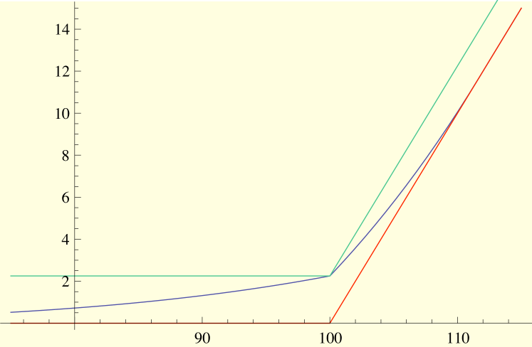
Figure 1. This figure displays the value function of the perpetual $\delta$-penalty call option for $r\leq d$ along with the immediate exercise and cancellation values. The penalty is such that value function has increasing derivative at $K$. Parameter values are $r=0.01,d=0.09$, $\sigma=0.20$, $K=100$, $k^{*}=111.7641$, and $\delta=2.25$.

Proof.

Suppose $0<\delta<\delta^{*}$. We propose that the value function is $r$-harmonic on the set $(0,K)\cup(K,k^{*})$, satisfies the smooth fit condition at $k^{*}$ and takes the value $\delta$ at the strike price $K$. Specifically, consider the boundary value problem

(3.3) $$\begin{split}\mathcal{L}v(x)=rv(x);\ v(K)=\delta,\ \lim_{x\downarrow 0}v(x)=0,\ \ x\in(0,K)\end{split}$$

where $\mathcal{L}:=(r-d)x\frac{\mathrm{d}}{\mathrm{d}x}+\frac{1}{2}\sigma^{2}x^{2}\frac{\mathrm{d}^{2}}{\mathrm{d}x^{2}}$. Let $v_{y}$ denote the derivative with respect to the parameter $y$. Solving this problem yields,

(3.4) $$\begin{split}v(x)&=\delta\left(\frac{x}{K}\right)^{\frac{\lambda}{\sigma}-\kappa}\ \text{for}\ x\in(0,K)\end{split}$$

Now consider the problem

(3.5) $$\begin{split}\mathcal{L}v(x)=rv(x);\ v(K)=\delta,v(k^{*})=(k^{*}-K)^{+},v_{x}(k^{*})=1,\ x\in(K,k^{*})\end{split}$$

The solution to this problem is

(3.6) $$v(x)=(k^{*}-K)\left(\frac{k^{*}}{x}\right)^{\kappa}\frac{\left(\frac{K}{x}\right)^{-\frac{\lambda}{\sigma}}-\left(\frac{K}{x}\right)^{\frac{\lambda}{\sigma}}}{\left(\frac{k^{*}}{K}\right)^{\frac{\lambda}{\sigma}}-\left(\frac{k^{*}}{K}\right)^{-\frac{\lambda}{\sigma}}}+\delta\left(\frac{K}{x}\right)^{\kappa}\frac{\left(\frac{k^{*}}{x}\right)^{\frac{\lambda}{\sigma}}-\left(\frac{k^{*}}{x}\right)^{-\frac{\lambda}{\sigma}}}{\left(\frac{k^{*}}{K}\right)^{\frac{\lambda}{\sigma}}-\left(\frac{k^{*}}{K}\right)^{-\frac{\lambda}{\sigma}}}\ \text{for}\ x\in(K,k^{*})$$

where $k^{*}$ satisfies the following equation

(3.7) $$\begin{split}&\left(\frac{k^{*}}{K}\right)^{\frac{2\lambda}{\sigma}}\left(-2\left(\frac{K}{k^{*}}\right)^{\kappa+\frac{\lambda}{\sigma}}\delta\lambda+(k^{*}-K)\left(\lambda-\kappa\sigma+\left(\frac{K}{k^{*}}\right)^{\frac{2\lambda}{\sigma}}(\lambda+\kappa\sigma)\right)\right)\\ &\quad=k^{*}\left(-1+\left(\frac{k^{*}}{K}\right)^{\frac{2\lambda}{\sigma}}\right)\sigma.\end{split}$$

Simple calculations, using the fact that $r\leq d$, show that $v(x)$ is an increasing, convex function on $(0,K)$. Before establishing that $v(x)$ is an increasing, convex function on $(K,k^{*})$, we first analyze its behavior at the strike price $K$. The solution $v(x)$ of the boundary value problem is continuous but is not necessarily differentiable at $K$. The following estimates show that the left-hand derivative is no larger than the right-hand derivative at $K$. A non-decreasing derivative at $K$ requires

(3.8) $$\begin{split}\frac{2(k^{*}-K)\left(\frac{k^{*}}{K}\right)^{\kappa+\frac{\lambda}{\sigma}}\lambda-2\left(\frac{k^{*}}{K}\right)^{\frac{2\lambda}{\sigma}}\delta\ \lambda}{\left(-1+\left(\frac{k^{*}}{K}\right)^{\frac{2\lambda}{\sigma}}\right)K\ \sigma}\geq 0\end{split}$$

Note the denominator is positive since $k^{*}\geq K$ and $\frac{2\lambda}{\sigma}\geq 0$. Hence, the derivative will be increasing at $K$ if the following holds

(3.9) $$\begin{split}(k^{*}-K)\left(\frac{k^{*}}{K}\right)^{\kappa+\frac{\lambda}{\sigma}}-\left(\frac{k^{*}}{K}\right)^{\frac{2\lambda}{\sigma}}\delta&\geq 0\ \Leftrightarrow\\ (k^{*}-K)\left(\frac{k^{*}}{K}\right)^{\kappa}-\left(\frac{k^{*}}{K}\right)^{\frac{\lambda}{\sigma}}\delta&\geq 0\end{split}$$

The left-side of this inequality is a decreasing, linear function of $\delta$. Thus, the condition on $\delta$ which guarantees the left-hand derivative is no larger than the right-hand derivative at $K$ is

(3.10) $$\begin{split}\delta\leq(k^{*}-K)\left(\frac{K}{k^{*}}\right)^{\frac{\lambda}{\sigma}-\kappa}\end{split}$$

Interestingly, the assumption $0<\delta<\delta^{*}$ guarantees (3.10) holds. One way in which to see this is to view $\delta$ as a function of $k^{*}$ in $(\ref{FOC1})$. Indeed, the function $\delta(k^{*})$ is a continuous, increasing function such that $\delta(K)=0$ and $\delta(b)=v^{c}(K)$. From this viewpoint and using this information, $(\ref{IncDeriv})$ will hold if

(3.11) $$\begin{split}f(x)&:=(x-K)\left(\frac{K}{x}\right)^{\frac{\lambda}{\sigma}-\kappa}\\ &\quad\quad+\frac{\left(\frac{K}{x}\right)^{-\frac{\lambda+\kappa\sigma}{\sigma}}\left(x\left(1-\left(\frac{x}{K}\right)^{\frac{-2\lambda}{\sigma}}\right)\sigma-(s-K)\left(\lambda-\kappa\sigma+\left(\frac{K}{x}\right)^{\frac{2\lambda}{\sigma}}(\lambda+\kappa\sigma)\right)\right)}{2\lambda}\\ &\geq 0,\ x\in[K,b]\end{split}$$

The function $f(x)$ is obtained by substituting the representation for $\delta$ in terms of $k^{*}$ into (3.10) and then subtracting this term from each side of the inequality. Details of the proof that $f(x)\geq 0$ for $x\in[K,b]$ are included in Section 7.
Continuing with the analysis of $v(x)$, its derivative on $(K,k^{*})$ (see formula $(\ref{dr-other})$) is

(3.12) $$\begin{split}&\left(\frac{1}{\left(-1+\left(\frac{k^{*}}{K}\right)^{\frac{2\lambda}{\sigma}}\right)x\sigma}\right)\times\Bigg{(}\left(\frac{k^{*}}{K}\right)^{\frac{\lambda}{\sigma}}\left(\frac{k^{*}}{x}\right)^{-\frac{\lambda}{\sigma}}\left(\frac{K}{x}\right)^{-\frac{\lambda}{\sigma}}\\ &\quad\Bigg{(}-\left(\frac{K}{x}\right)^{\kappa+\frac{\lambda}{\sigma}}\delta\left(\lambda-\kappa\sigma+\left(\frac{k^{*}}{x}\right)^{\frac{2\lambda}{\sigma}}\left(\lambda+\kappa\sigma\right)\right)\\ &\quad+(k^{*}-K)\left(\frac{k^{*}}{x}\right)^{\kappa+\frac{\lambda}{\sigma}}\left(\lambda-\kappa\sigma+\left(\frac{K}{x}\right)^{\frac{2\lambda}{\sigma}}(\lambda+\kappa\sigma)\right)\Bigg{)}\Bigg{)}\end{split}$$

Note the first line in (3.12) above has four factors that are all positive. Since $\delta\leq(k^{*}-K)\left(\frac{K}{k^{*}}\right)^{\frac{\lambda}{\sigma}-\kappa}$, the expression in the remaining two lines of the above derivative is greater than or equal to

(3.13) $$\begin{split}&(k^{*}-K)\Bigg{(}-\left(\frac{K}{k^{*}}\right)^{-\kappa+\frac{\lambda}{\sigma}}\left(\frac{K}{x}\right)^{\kappa+\frac{\lambda}{\sigma}}\left(\lambda-\kappa\sigma+\left(\frac{k^{*}}{x}\right)^{\frac{2\lambda}{\sigma}}\left(\lambda+\kappa\sigma\right)\right)\\ &\quad+\left(\frac{k^{*}}{x}\right)^{\kappa+\frac{\lambda}{\sigma}}\left(\lambda-\kappa\sigma+\left(\frac{K}{x}\right)^{\frac{2\lambda}{\sigma}}(\lambda+\kappa\sigma)\right)\Bigg{)}\end{split}$$

Since $k^{*}\geq K$, consider only the second factor in the above representation. Now taking a derivative yields

(3.14) $$\begin{split}\frac{2k^{*}\left(\frac{K}{k^{*}}\right)^{\frac{2\lambda}{\sigma}}\left(\frac{k^{*}}{x}\right)^{-1+\frac{2\lambda}{\sigma}}\lambda(\lambda+\kappa\sigma)}{x^{2}\sigma}-\frac{2K\left(\frac{K}{x}\right)^{-1+\frac{2\lambda}{\sigma}}\lambda(\lambda+\kappa\sigma)}{x^{2}\sigma}&=0\end{split}$$

Thus, the second factor is a constant function of $x$. Substituting the value at $x=k^{*}$ into the second factor produces

(3.15) $$\begin{split}-\left(-1+\left(\frac{K}{k^{*}}\right)^{\frac{2\lambda}{\sigma}}(\lambda-\kappa\sigma)\right)\geq 0\end{split}$$

We conclude that $v(x)$ is increasing on $(K,k^{*})$. Additionally, using the fact that $v(x)$ is $r$-harmonic on $(K,k^{*})$, $r\leq d$, $v_{x}(x)\geq 0$, and $v(x)>0$, we have

(3.16) $$\begin{split}v_{xx}=\frac{2}{\sigma^{2}x^{2}}\left[(d-r)xv_{x}(x)+rv(x)\right]>0\end{split}$$

Thus, $v(x)$ is convex on $(K,k^{*})$. At this point, we conclude $v(x)$ is a convex function on $(0,\infty)$. Summing up, $v(x)\in\mathcal{C}^{2}(0,K)\cup\mathcal{C}^{1}(K,\infty)\cup\mathcal{C}^{2}[(K,\infty)\setminus\{k^{*}\}]$, $v(x)$ is $r$-harmonic on $(0,K)\cup(K,k^{*})$ and $v(x)$ is $r$-superharmonic on $(k^{*},\infty)$. Using these results, the following argument by Kyprianou (2004) proves that the solution to the boundary value problem is, indeed, the value function. Let $\sigma_{k^{*}}:=\inf{\{t\geq 0:X_{t}\geq k^{*}\}}$ and $\tau_{K}:=\inf{\{t\geq 0:X_{t}=K\}}$.

(3.17) $$\begin{split}v(x)&\leq\inf_{\tau\in\mathcal{S}_{0,\infty}}\mathbb{E}_{x}[e^{-r(\tau\wedge\sigma_{k^{*}})}v(X_{\tau\wedge\sigma_{k^{*}}})]\\ &\leq\inf_{\tau\in\mathcal{S}_{0,\infty}}\mathbb{E}_{x}[e^{-r(\tau\wedge\sigma_{k^{*}})}\left((X_{\sigma_{{k^{*}}}}-K)^{+}1_{\{\sigma_{k^{*}}\leq\tau\}}+((X_{\tau}-K)^{+}+\delta)1_{\{\tau<\sigma_{k^{*}}\}}\right)]\\ &\leq\sup_{\sigma\in\mathcal{S}_{0,\infty}}\inf_{\tau\in\mathcal{S}_{0,\infty}}\mathbb{E}_{x}[e^{-r(\tau\wedge\sigma)}\left((X_{\sigma}-K)^{+}1_{\{\sigma\leq\tau\}}+((X_{\tau}-K)^{+}+\delta)1_{\{\tau<\sigma\}}\right)]\\ &\leq\sup_{\sigma\in\mathcal{S}_{0,\infty}}\mathbb{E}_{x}[e^{-r(\tau_{K}\wedge\sigma)}\left((X_{\sigma}-K)^{+}1_{\{\sigma\leq\tau_{K}\}}+((X_{\tau_{K}}-K)^{+}+\delta)1_{\{\tau_{K}<\sigma\}}\right)]\\ &\leq\sup_{\sigma\in\mathcal{S}_{0,\infty}}\mathbb{E}_{x}[e^{-r(\tau_{K}\wedge\sigma)}v(X_{\tau_{K}\wedge\sigma})]\\ &\leq v(x)\end{split}$$

The first inequality follows since $v(x)$ is $r$-harmonic on $(0,K)\cup(K,k^{*})$. The second inequality follows since $v(x)$ satisfies $(x-K)^{+}\leq v(x)\leq(x-K)^{+}+\delta$. The third and fourth inequalities follow using the definition of the supremum and infimum respectively. The fifth inequality holds using the same bound as in the second inequality. The final inequality follows since $v(x)$ is $r$-superharmonic on $(k^{*},\infty)$. Note, the order of the supremum and infimum can be switched by establishing the above inequalities in reverse. This completes the proof. ∎

4. Valuation when $r>d$

Here we assume the interest rate $r$ is strictly larger than the constant dividend yield $d$ of the underlying asset. It seems reasonable to conjecture that the value function is identical to the solution found in the prior parameter case. However, Figure 2 disproves this hypothesis since the proposed value function defined in Proposition 3.1 does not satisfy the basic inequality,

(4.1) $$(x-K)^{+}\leq V(x)\leq(x-K)^{+}+\delta$$

Figure 2. $\delta$-penalty call option: This figure shows that the proposed value function (blue line) violates the upper bound on the value (green line) on the interval $(K,k^{*})$. Parameter values are $r=0.06,d=0.03$, $\sigma=0.20$, $K=100$, $k^{*}=272.4404$, and $\delta=10$.

With this information, it seems likely that the cancellation region is of the form $[K,h],\ h\neq K$. The following argument suggests why the closed region should be connected. Suppose that for $x<y$, $V(x)=(x-K)^{+}+\delta$ and $V(y)=(y-K)^{+}+\delta$ and that for some $z$ where $x<z<y$, $V(z)<(z-K)^{+}+\delta$. Since $V$ is a continuous function with derivative satisfying $0\leq V_{x}\leq 1$ (see Proposition 2.1), we have an immediate contradiction.
It is well-known that the fundamental solutions of the ordinary second order differential equation $\mathcal{L}v-rv=0$ are $\psi(x)=x^{\eta}$ and $\varphi(x)=x^{\nu}$, where

(4.2) $$\begin{split}\eta&=\frac{1}{2}-\frac{r-d}{\sigma^{2}}+\sqrt{\left(\frac{1}{2}-\frac{r-d}{\sigma^{2}}\right)^{2}+\frac{2r}{\sigma^{2}}}>0\\ \nu&=\frac{1}{2}-\frac{r-d}{\sigma^{2}}-\sqrt{\left(\frac{1}{2}-\frac{r-d}{\sigma^{2}}\right)^{2}+\frac{2r}{\sigma^{2}}}<0\end{split}$$

are the roots of the equation $\sigma^{2}(y-1)y+2(r-d)=2r$. In addition, $\psi^{\prime}(x)-\varphi(x)-\varphi^{\prime}(x)\psi(x)=BS^{\prime}(x)$. Here, $B>0$ denotes the Wronskian of the fundamental solutions $(\psi(x)$, $\varphi(x))$, and $S^{\prime}(x)$ is the density of the scale function $S$, where

(4.3) $$\begin{split}S(x):=\int_{c}^{x}\exp\left(-2\int_{c}^{y}\frac{(r-d)z}{\sigma^{2}z^{2}}\mathrm{d}z\right)\mathrm{d}y,\ \text{for}\ x\in(0,\infty)\end{split}$$

where $c$ is an arbitrary fixed element of $(0,\infty)$. The functions

(4.4) $$\begin{split}\hat{\psi}_{h}(x):=\psi(x)-\frac{\psi(h)}{\varphi(h)}\varphi(x)\\ \hat{\varphi}_{k}(x):=\varphi(x)-\frac{\varphi(k)}{\psi(k)}\psi(x)\end{split}$$

are the fundamental solutions of $\mathcal{L}v-rv=0$ defined on the domain of the differential operator of the killed diffusion $\{X_{t}:t\in[0,\lambda_{h}\wedge\lambda_{k})\}$; $\lambda_{a}:=\inf\{t\geq 0:X_{t}=a\}$. Finally, the density of the speed measure of $X_{t}$ is $m^{\prime}(y)=\frac{2}{\sigma^{2}y^{2}S^{\prime}(y)}$ (see Borodin, Salminen (1996) Chapter 2 for details).
Using the above information, we now present the main result of this section. Let $\sigma_{k^{*}}:=\inf{\{t\geq 0:X_{t}\geq k^{*}\}}$, and $\tau_{[K,h^{*}]}:=\inf{\{t\geq 0:K\leq X_{t}\leq h^{*}\}}$ where $k^{*}$ and $h^{*}$ are defined below.

Theorem 4.1.

Suppose $r\geq d$. For $0<\delta\leq\delta^{*}$, the perpetual $\delta$-penalty call option has value process $V(X_{t})$ with

(4.5) $$\begin{split}V(x)=\begin{cases}x-K&\textrm{if}\ x\in[k^{*},\infty)\\ (k^{*}-K)^{+}\mathbb{E}_{x}[e^{-r\sigma_{k^{*}}}1_{\{\sigma_{k^{*}}\leq\tau_{[K,h^{*}]}\}}]\\ \quad+((h^{*}-K)^{+}+\delta)\mathbb{E}_{x}[e^{-r\tau_{[K,h^{*}]}}1_{\{\tau_{[K,h^{*}]}<\sigma_{k^{*}}\}}]&\textrm{if}\ x\in(h^{*},k^{*})\\ (x-K)+\delta&\textrm{if}\ x\in[K,h^{*}]\\ \delta\ \mathbb{E}_{x}[e^{-r\tau_{[K,h^{*}]}}]&\textrm{if}\ x\in(0,K)\end{cases}\end{split}$$

where the pair $(h^{*},k^{*})$ both satisfies the equations

(4.6) $$\begin{split}\frac{1}{S^{\prime}(h^{*})}\hat{\varphi}_{k^{*}}(h^{*})-\frac{\hat{\varphi}^{\prime}_{k^{*}}(h^{*})}{S^{\prime}(h^{*})}((h^{*}-K)^{+}+\delta)&=B\frac{(k^{*}-K)^{+}}{\psi(k^{*})}\\ \frac{1}{S^{\prime}(k^{*})}\hat{\psi}_{h^{*}}(k^{*})-\frac{\hat{\psi}^{\prime}_{h^{*}}(k^{*})}{S^{\prime}(k^{*})}(k^{*}-K)^{+}&=-B\frac{(h^{*}-K)^{+}+\delta}{\varphi(h^{*})}\end{split}$$

and the inequalities $K<h^{*}<k^{*}$. Thus, the value function $V$ is continuous for all $x>0$ and is differentiable at $h^{*}$ and $k^{*}$ (by (4.6)).

The distinctive feature of this valuation formula is that the writer’s termination region is the interval $[K,h^{*}]$ for $h^{*}>K$ rather than simply the singleton $\{K\}$. Intuition for this result arises by examining the instantaneous gain to the writer for terminating the contract at time $t$. A positive value for $rK-dX_{t}-\delta$ provides an incentive for the writer to terminate the call option. This may occur when the interest rate $r$ is larger than the dividend rate $d$. If such a situation develops, then immediate termination by the writer might be preferable for some asset values strictly greater than the strike price (e.g. see Figure 3). Before proving Theorem 4.1, we state a useful lemma concerning the pair $(h^{*},k^{*})$ whose proof appears in Section 7.

Lemma 4.2.

A pair $(h^{*},k^{*})$ solving the equations (4.6) with $K<h^{*}<k^{*}$ satisfies $h^{*}<\frac{r(K-\delta)}{d}$ and $k^{*}>\frac{r}{d}K$.

We now prove the main result.

Proof.

(of Theorem 4.1) Recall, $V^{*}(x)$ denotes the value function from (2.3). Here, we intend to show $V^{*}(x)=V(x)$ for $x>0$ by establishing the following sequence of relations

(4.7) $$\begin{split}V(x)&\geq\sup_{\sigma\in\mathcal{S}_{0,\infty}}\mathbb{E}_{x}[e^{-r(\sigma\wedge\tau_{[K,h^{*}]})}\{((X_{\tau_{[K,h^{*}]}}-K)^{+}+\delta)1_{\{\tau_{[K,h^{*}]}<\sigma\}}+(X_{\sigma}-K)^{+}1_{\{\sigma\leq\tau_{[K,h^{*}]}\}}\}]\\ &\geq\inf_{\tau\in\mathcal{S}_{0,\infty}}\sup_{\sigma\in\mathcal{S}_{0,\infty}}\mathbb{E}_{x}[e^{-r(\sigma\wedge\tau)}\{((X_{\tau}-K)^{+}+\delta)1_{\{\tau<\sigma\}}+(X_{\sigma}-K)^{+}1_{\{\sigma\leq\tau\}}\}]\\ &\geq\sup_{\sigma\in\mathcal{S}_{0,\infty}}\inf_{\tau\in\mathcal{S}_{0,\infty}}\mathbb{E}_{x}[e^{-r(\sigma\wedge\tau)}\{((X_{\tau}-K)^{+}+\delta)1_{\{\tau<\sigma\}}+(X_{\sigma}-K)^{+}1_{\{\sigma\leq\tau\}}\}]\\ &\geq V(x)\end{split}$$

Notice that justification of the the first and last relations will complete the proof. We begin by establishing the first inequality. By (4.5) and (4.6), $V$ is continuously differentiable everywhere except at $K$, and twice continuously differentiable everywhere except at $K$, $h^{*}$, and $k^{*}$. Using the change-of-variable formula with local time on curves (Peskir (2005) Remark 2.3) applied to $e^{-rt}V(X_{t})$, we obtain

(4.8) $$\begin{split}e^{-rt}V(X_{t})&=V(x)+\int_{0}^{t}(\mathcal{L}V-rV)(s,X_{s})1_{\{X_{s}\neq k^{*}\}\cap\{X_{s}\neq h^{*}\}\cap\{X_{s}\neq K\}}\mathrm{d}s\\ &\quad\quad+\int_{0}^{t}e^{-rs}\sigma X_{s}V_{x}(X_{s})1_{\{X_{s}\neq k^{*}\}\cap\{X_{s}\neq h^{*}\}\cap\{X_{s}\neq K\}}\mathrm{d}W_{s}\\ &\quad\quad\quad+\frac{1}{2}\int_{0}^{t}e^{-rs}(V_{x}(X_{s}+)-V_{x}(X_{s}-))1_{\{X_{s}=K\}}\mathrm{d}\ell^{K}_{s}(X)\end{split}$$

where $\ell^{c}_{s}(X)$ is the local time of $X$ at the curve $c$ given by

(4.9) $$\begin{split}\ell^{c}_{s}(X)=\lim_{\epsilon\downarrow 0}\frac{1}{2\epsilon}\int^{s}_{0}1_{\{c(v)-\epsilon<X_{v}<c(v)+\epsilon\}}\mathrm{d}[X]_{v}\end{split}$$

In the following, let $(\tau_{n})_{n=1}^{\infty}$ be a localizing sequence for the continuous local martingale,

(4.10) $$\int_{0}^{t}e^{-rs}\sigma X_{s}V_{x}(X_{s})1_{\{X_{s}\neq k^{*}\}\cap\{X_{s}\neq h^{*}\}\cap\{X_{s}\neq K\}}\mathrm{d}W_{s}$$

Let $x\in(h^{*},k^{*})$. Using the fact that $\mathcal{L}V=rV$ in $(h^{*},k^{*})$ and the optional sampling theorem, we know for each $n\geq 1$,

(4.11) $$\begin{split}\mathbb{E}_{x}[e^{-r(\tau_{[K,h^{*}]}\wedge\sigma_{k^{*}}\wedge\tau_{n})}V(X_{\tau_{[K,h^{*}]}\wedge\sigma_{k^{*}}\wedge\tau_{n}})]=V(x)\end{split}$$

Letting $n\rightarrow\infty$, we have by the bounded convergence theorem and the continuity of $V$,

(4.12) $$\begin{split}\mathbb{E}_{x}[e^{-r(\tau_{[K,h^{*}]}\wedge\sigma_{k^{*}})}V(X_{\tau_{[K,h^{*}]}\wedge\sigma_{k^{*}}})]=V(x)\end{split}$$

This same argument also shows that (4.12) holds for $x\in(0,K)$ since $\mathcal{L}V=rV$ there. Since (4.12) clearly holds when $x\in[K,h^{*}]$ and when $x\in[k^{*},\infty)$, we conclude (4.12) holds for all $x>0$. Using Lemma 4.2, we know for any $x\in[k^{*},\infty)$,

(4.13) $$(\mathcal{L}g_{1}-rg_{1})(x)=(r-d)x-r(x-K)=rK-dx<0$$

where $g_{1}(x):=(x-K)^{+}$. Therefore, for $x\in(h^{*},k^{*})$ and any $n\geq 1$,

(4.14) $$\begin{split}\mathbb{E}_{x}[e^{-r(\sigma\wedge\tau_{[K,h^{*}]}\wedge\tau_{n})}V(X_{\sigma\wedge\tau_{[K,h^{*}]}\wedge\tau_{n}})]\leq V(x)\end{split}$$

Thus, by Fatou’s lemma

(4.15) $$\begin{split}\mathbb{E}_{x}[e^{-r(\sigma\wedge\tau_{[K,h^{*}]})}V(X_{\sigma\wedge\tau_{[K,h^{*}]}})]\leq V(x)\end{split}$$

Using Lemma 7.4, we find

(4.16) $$\begin{split}&\mathbb{E}_{x}[e^{-r(\sigma\wedge\tau_{[K,h^{*}]})}\{((X_{\tau_{[K,h^{*}]}}-K)^{+}+\delta)1_{\{\tau_{[K,h^{*}]}<\sigma\}}+(X_{\sigma}-K)^{+}1_{\{\sigma\leq\tau_{[K,h^{*}]}\}}\}]\\ &\leq\mathbb{E}_{x}[e^{-r(\sigma\wedge\tau_{[K,h^{*}]})}V(X_{\sigma\wedge\tau_{[K,h^{*}]}})]\\ &\leq V(x)\end{split}$$

Taking the supremum over all stopping times $\sigma$ yields,

(4.17) $$\begin{split}&\sup_{\sigma\in\mathcal{S}_{0,\infty}}\mathbb{E}_{x}[e^{-r(\sigma\wedge\tau_{[K,h^{*}]})}\{((X_{\tau_{[K,h^{*}]}}-K)^{+}+\delta)1_{\{\tau_{[K,h^{*}]}<\sigma\}}+(X_{\sigma}-K)^{+}1_{\{\sigma\leq\tau_{[K,h^{*}]}\}}\}]\\ &\quad\leq V(x)\end{split}$$

Thus, the first inequality of (4.7) holds when $x\in(h^{*},k^{*})$. Continuing when $x\in(h^{*},k^{*})$, recall

(4.18) $$\begin{split}&\mathbb{E}_{x}[e^{-r(\tau_{[K,h^{*}]}\wedge\sigma_{k^{*}})}V(X_{\tau_{[K,h^{*}]}\wedge\sigma_{k^{*}}})]\\ &\quad=\mathbb{E}_{x}[e^{-r(\sigma_{k^{*}}\wedge\tau_{[K,h^{*}]})}\{((X_{\tau_{[K,h^{*}]}}-K)^{+}+\delta)1_{\{\tau_{[K,h^{*}]}<\sigma_{k^{*}}\}}+(X_{\sigma_{k^{*}}}-K)^{+}1_{\{\sigma_{k^{*}}\leq\tau_{[K,h^{*}]}\}}\}]\\ &\quad=V(x)\end{split}$$

Thus,

(4.19) $$\begin{split}V(x)&\geq\inf_{\tau\in\mathcal{S}_{0,\infty}}\mathbb{E}_{x}[e^{-r(\sigma_{k^{*}}\wedge\tau)}\{((X_{\tau}-K)^{+}+\delta)1_{\{\tau<\sigma_{k^{*}}\}}+(X_{\sigma_{k^{*}}}-K)^{+}1_{\{\sigma_{k^{*}}\leq\tau\}}\}]\end{split}$$

We now establish the opposite inequality. Using Lemma 4.2, for any $x\in\left(K,\frac{r(K-\delta)}{d}\right)$,

(4.20) $$(\mathcal{L}g_{2}-rg_{2})(x)=(r-d)x-r((x-K)+\delta)=rK-dx-r\delta>0$$

where $g_{2}(x):=(x-K)^{+}+\delta$. Therefore, for $x\in(h^{*},k^{*})$ and $n\geq 1$ the optional sampling theorem yields for any $\tau\in\mathcal{S}_{0,\infty}$,

(4.21) $$\begin{split}\mathbb{E}_{x}[e^{-r(\tau\wedge\sigma_{k^{*}}\wedge\tau_{n})}V(X_{\tau\wedge\sigma_{k^{*}}\wedge\tau_{n}})]\geq V(x)\end{split}$$

By Lemma 7.4 we know,

(4.22) $$\begin{split}\mathbb{E}_{x}[e^{-r(\tau\wedge\sigma_{k^{*}}\wedge\tau_{n})}V(X_{\tau\wedge\sigma_{k^{*}}\wedge\tau_{n}})]&\leq\mathbb{E}_{x}[e^{-r(\tau\wedge\sigma_{k^{*}}\wedge\tau_{n})}[((X_{\tau\wedge\tau_{n}}-K)^{+}+\delta)1_{\{\tau\wedge\tau_{n}<\sigma_{k^{*}}\}}\\ &\quad\quad+(X_{\sigma_{k^{*}}}-K)^{+}1_{\{\sigma_{k^{*}}\leq\tau\wedge\tau_{n}\}}]]\end{split}$$

Then, two applications of the bounded convergence theorem (while recalling the continuity of $V$) yields

(4.23) $$\begin{split}V(x)&\leq\mathbb{E}_{x}[e^{-r(\tau\wedge\sigma_{k^{*}})}V(X_{\tau\wedge\sigma_{k^{*}}})]\\ &\leq\mathbb{E}_{x}[e^{-r(\tau\wedge\sigma_{k^{*}})}[((X_{\tau}-K)^{+}+\delta)1_{\{\tau<\sigma_{k^{*}}\}}+(X_{\sigma_{k^{*}}}-K)^{+}1_{\{\sigma_{k^{*}}\leq\tau\}}]]\end{split}$$

Hence,

(4.24) $$\begin{split}V(x)&\leq\inf_{\tau\in\mathcal{S}_{0,\infty}}\mathbb{E}_{x}[e^{-r(\tau\wedge\sigma_{k^{*}})}[((X_{\tau}-K)^{+}+\delta)1_{\{\tau<\sigma_{k^{*}}\}}+(X_{\sigma_{k^{*}}}-K)^{+}1_{\{\sigma_{k^{*}}\leq\tau\}}]]\end{split}$$

Thus, the opposite equality has been established and the following relations hold.

(4.25) $$\begin{split}V(x)&=\inf_{\tau\in\mathcal{S}_{0,\infty}}\mathbb{E}_{x}[e^{-r(\tau\wedge\sigma_{k^{*}})}[((X_{\tau}-K)^{+}+\delta)1_{\{\tau<\sigma_{k^{*}}\}}+(X_{\sigma_{k^{*}}}-K)^{+}1_{\{\sigma_{k^{*}}\leq\tau\}}]]\\ &\leq\sup_{\sigma\in\mathcal{S}_{0,\infty}}\inf_{\tau\in\mathcal{S}_{0,\infty}}\mathbb{E}_{x}[e^{-r(\tau\wedge\sigma)}[((X_{\tau}-K)^{+}+\delta)1_{\{\tau<\sigma\}}+(X_{\sigma}-K)^{+}1_{\{\sigma\leq\tau\}}]]\\ \end{split}$$

This completes the justification and $V(x)=V^{*}(x)$ when $x\in(h^{*},k^{*})$ as desired.
Suppose $x\in(0,K)$. Using the fact that $\mathcal{L}V-rV$ in $(0,K)$ and the optional sampling theorem, we know for each $n\geq 1$ and any $\sigma\in\mathcal{S}_{0,\infty}$,

(4.26) $$\begin{split}\mathbb{E}_{x}[e^{-r(\tau_{[K,h^{*}]}\wedge\sigma\wedge\tau_{n})}V(X_{\tau_{[K,h^{*}]}\wedge\sigma\wedge\tau_{n}})]=V(x)\end{split}$$

An application of the bounded convergence theorem (while recalling the continuity $V$) followed by Lemma 7.4 produces

(4.27) $$\begin{split}V(x)\geq\sup_{\sigma\in\mathcal{S}_{0,\infty}}\mathbb{E}_{x}[e^{-r(\sigma\wedge\tau_{[K,h^{*}]})}\{((X_{\tau_{[K,h^{*}]}}-K)^{+}+\delta)1_{\{\tau_{[K,h^{*}]}<\sigma\}}+(X_{\sigma}-K)^{+}1_{\{\sigma\leq\tau_{[K,h^{*}]}\}}\}]\ \end{split}$$

Thus, the first inequality in (4.7) holds. In addition, since $\tau_{[K,h^{*}]}<\sigma_{k^{*}}$, we have

(4.28) $$\begin{split}V(x)&=\mathbb{E}_{x}[e^{-r(\tau_{[K,h^{*}]}\wedge\sigma_{k^{*}})}V(X_{\tau_{[K,h^{*}]}\wedge\sigma_{k^{*}}})]\\ &\quad=\mathbb{E}_{x}[e^{-r(\sigma_{k^{*}}\wedge\tau_{[K,h^{*}]})}\{((X_{\tau_{[K,h^{*}]}}-K)^{+}+\delta)1_{\{\tau_{[K,h^{*}]}<\sigma_{k^{*}}\}}+(X_{\sigma_{k^{*}}}-K)^{+}1_{\{\sigma_{k^{*}}\leq\tau_{[K,h^{*}]}\}}\}]\end{split}$$

which implies

(4.29) $$\begin{split}V(x)&\geq\inf_{\tau\in\mathcal{S}_{0,\infty}}\mathbb{E}_{x}[e^{-r(\sigma_{k^{*}}\wedge\tau)}\{((X_{\tau}-K)^{+}+\delta)1_{\{\tau<\sigma_{k^{*}}\}}+(X_{\sigma_{k^{*}}}-K)^{+}1_{\{\sigma_{k^{*}}\leq\tau\}}\}]\end{split}$$

The same argument used when $x\in(h^{*},k^{*})$ applies here to show that the opposite inequality in (4.29) holds. Therefore, $V^{*}(x)=V(x)$ when $x\in(0,K)$.

Suppose $x\in[K,h^{*}]$. Using (4.12) and the fact that $\tau_{[K,h^{*}]}=0$, for any stopping time $\sigma\in\mathcal{S}_{0,\infty}$,

(4.30) $$\begin{split}V(x)&\geq\mathbb{E}_{x}[e^{-r(\sigma\wedge\tau_{[K,h^{*}]})}\{((X_{\tau_{[K,h^{*}]}}-K)^{+}+\delta)1_{\{\tau_{[K,h^{*}]}<\sigma\}}+(X_{\sigma}-K)^{+}1_{\{\sigma\leq\tau_{[K,h^{*}]}\}}\}]\end{split}$$

Note that equality in (4.30) actually holds. Now, taking the supremum over all stopping times in (4.30) yields the first inequality in (4.7). Again using (4.12) and $\tau_{[K,h^{*}]}=0$ yields,

(4.31) $$\begin{split}V(x)&\geq\inf_{\tau\in\mathcal{S}_{0,\infty}}\mathbb{E}_{x}[e^{-r(\sigma_{k^{*}}\wedge\tau)}\{((X_{\tau}-K)^{+}+\delta)1_{\{\tau<\sigma_{k^{*}}\}}+((X_{\sigma_{k^{*}}}-K)^{+})1_{\{\sigma_{k^{*}}\leq\tau\}}\}]\end{split}$$

The same argument used when $x\in(h^{*},k^{*})$ applies here to show the opposite inequality in (4.31). Thus, $V(x)=V^{*}(x)$.
Finally, suppose $x\in[k^{*},\infty)$. By Lemma 7.4, we know

(4.32) $$\begin{split}&\mathbb{E}_{x}[e^{-r(\sigma\wedge\tau_{[K,h^{*}]})}\{((X_{\tau_{[K,h^{*}]}}-K)^{+}+\delta)1_{\{\tau_{[K,h^{*}]}<\sigma\}}+(X_{\sigma}-K)^{+}1_{\{\sigma\leq\tau_{[K,h^{*}]}\}}\}]\\ \quad&\leq\mathbb{E}_{x}[e^{-r(\sigma\wedge\tau_{[K,h^{*}]}}V(X_{\sigma\wedge\tau_{[K,h^{*}]}})]\end{split}$$

Using Lemma 4.2 and the optional sampling theorem for any $\sigma\in\mathcal{S}_{0,\infty}$ and $n\geq 1$, we have

(4.33) $$\begin{split}\mathbb{E}_{x}[e^{-r(\sigma\wedge\tau_{[K,h^{*}]}\wedge\tau_{n})}V(X_{\sigma\wedge\tau_{[K,h^{*}]}\wedge\tau_{n}})]&\leq V(x)\end{split}$$

By Fatou’s Lemma and the continuity of $V$, we conclude

(4.34) $$\begin{split}&\mathbb{E}_{x}[e^{-r(\sigma\wedge\tau_{[K,h^{*}]})}\{((X_{\tau_{[K,h^{*}]}}-K)^{+}+\delta)1_{\{\tau_{[K,h^{*}]}<\sigma\}}+(X_{\sigma}-K)^{+}1_{\{\sigma\leq\tau_{[K,h^{*}]}\}}\}]\\ \quad&\leq V(x)\end{split}$$

Taking the supremum over all stopping times $\sigma$ yields the first inequality in (4.7). Since $\sigma_{k^{*}}=0$, for any stopping time $\tau\in\mathcal{S}_{0,\infty}$,

(4.35) $$\begin{split}V(x)&=\mathbb{E}_{x}[e^{-r(\sigma_{k^{*}}\wedge\tau)}\{((X_{\tau}-K)^{+}+\delta)1_{\{\tau<\sigma_{k^{*}}\}}+((X_{\sigma_{k^{*}}}-K)^{+})1_{\{\sigma_{k^{*}}\leq\tau\}}\}]\end{split}$$

Thus, we have

(4.36) $$\begin{split}V(x)&=\inf_{\tau\in\mathcal{S}_{0,\infty}}\mathbb{E}_{x}[e^{-r(\sigma_{k^{*}}\wedge\tau)}\{((X_{\tau}-K)^{+}+\delta)1_{\{\tau<\sigma_{k^{*}}\}}+((X_{\sigma_{k^{*}}}-K)^{+})1_{\{\sigma_{k^{*}}\leq\tau\}}\}]\end{split}$$

Thus, $V(x)=V^{*}(x)$. This completes the proof. ∎

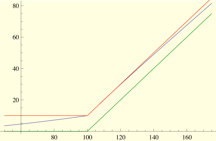
Figure 3. This figure displays the value function for the $\delta$-penalty call option and the immediate exercise value functions on the interval $[50,175]$. Parameter values are: $r=0.02$, $d=0.01$, $\delta=10$, $\sigma=0.2$, $h^{*}=107.50$, $k^{*}=329.90$.

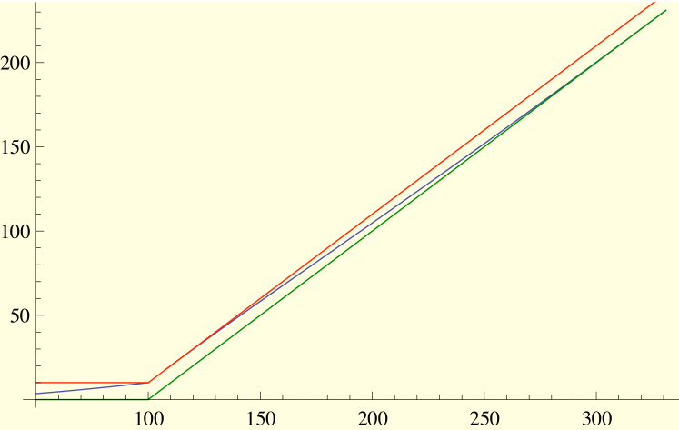
Figure 4. This figure displays the value function for the $\delta$-penalty call option and the immediate exercise value functions on the interval $[50,330]$. Parameter values are: $r=0.02$, $d=0.01$, $\delta=10$, $\sigma=0.2$, $h^{*}=107.50$, $k^{*}=329.90$.

5. Numerical Results

This section presents numerical results pertaining to the $\delta$-penalty call option when $r>d$. Recall, when the interest rate exceeds the dividend yield, the price function is not always a convex function for all values of the underlying asset.
Figure 3 displays the value function for the $\delta$-penalty call option and the immediate exercise value functions on $[50,175]$ with parameter values: $r=0.02$, $d=0.01$, $\sigma=0.2$, $K=100$, $\delta=10$. We see that the value function smoothly joins the upper immediate exercise value function at $h^{*}=107.50$. Thus, the immediate cancellation region is the interval $[100,107.50]$. In addition, Figure 4 shows that the value function smoothly joins the lower immediate exercise value function at $k^{*}=329.90$. Hence, the immediate exercise region consists of the interval $[329.90,\infty)$.
Our analysis in the previous section and the value function featured in Figure 3 highlight the fact that the price of the $\delta$-penalty call option need not be a convex function of the underlying asset even though the payoff is convex. This result, though striking, is not unexpected from previous analysis done on game-style options (see e.g. Ekström (2006)). Moreover, our results show that the $\delta$-penalty call option is not necessarily non-decreasing in the volatility parameter. Indeed, Table 1 shows that for asset values of $X=120,130,140,150$, the $\delta$-penalty call option is decreasing in volatility for model parameters $r=0.02$, $d=0.01$, $\delta=10$, $K=100$. Note this phenomenon occurs near non-convex pieces of the value function. Not surprisingly, this quality of the price disappears as asset values approach $k^{*}$ and the value function switches to being convex. Indeed, Table 1 indicates that prices are increasing in volatility when $X=280$ and $X=290$. This numerical example highlights the close relationship between the convexity of the price function and its monotonicity with respect to the volatility parameter.
The price savings over a perpetual American Call option can be substantial. Since optimal cancellation occurs in an interval with the strike as the left endpoint, we would expect the greatest savings to occur close to this interval. Indeed, we see from Table 1 that the cost savings to the investor of a $\delta$-penalty call option is greatest at $X=120$ for any fixed $\sigma$ value. In fact, for $X=120$ and $\sigma=0.15$, the cost savings of $26.5132$ represents nearly $89\%$ of the option value and nearly $47\%$ of the regular American call option value.

Table: Perpetual Cancellable Call, Perpetual American Call, Savings premia

Asset Volatility Canc. Call Amer. Call Savings Premia

Table 1. Note: Columns 1 and 2 give the underlying asset price $X$ and its return volatility $\sigma$. Columns 3 and 4 provide the $\delta$-penalty Call Option price and the Perpetual American Call Option price. Column 5 is the savings from purchasing a $\delta$-penalty call over a Perpetual American call. Parameter values are $r=0.02$, $d=0.01$, $\delta=10$, $K=100,$. $\sigma=0.15\ \Rightarrow h^{*}=115.0460,\ k^{*}=294.5790$. $\sigma=0.20\ \Rightarrow h^{*}=107.4860,\ k^{*}=329.8960$. $\sigma=0.25\ \Rightarrow h^{*}=101.0210,\ k^{*}=365.7920$.

6. Conclusion

The above discussion presents the valuation of the perpetual $\delta$-penalty call option. This analysis follows the work done in Kyprianou (2004) with respect to the perpetual $\delta$-penalty put option. We find that the solution to the problem differs considerably depending on the relative values of the interest rate and dividend yield for the underlying asset. Specifically, when $r\leq d$, analogous arguments to Kyprianou (2004) identify the explicit solution to the valuation problem. Namely, the value of the claim corresponds to its price under the policy of exercising at the first time the underlying asset reaches an optimally chosen value $k^{*}$ and under the policy of terminating the contract when the asset value first reaches the strike price $K$. In addition, the value function is a convex function of the underlying asset price. When $r>d$, the optimal cancellation region no longer is the singleton $\{K\}$ in general. Instead, it consists of an interval of the form $[K,h^{*}]$; where $h^{*}$ must be determined as part of the solution. We show that $h^{*}$ and $k^{*}$ respects two natural bounds. Namely, the optimal termination point satisfies $h^{*}\leq\frac{r(K-\delta)}{d}$ and the optimal exercise point satisfies $k^{*}\geq\frac{r}{d}K$. In addition, smooth-pasting holds both at the holder’s optimal exercise boundary value $k^{*}$ and the writer’s cancellation value $h^{*}$. This striking result implies that the price is not a convex function for all values of the underlying asset. Further, numerical solutions for the valuation problem show that the value function is not necessarily non-decreasing in the volatility parameter. This phenomenon directly relates to the existence of non-convex pieces of the value function. Finally, we observe significant price savings over the perpetual call option. This savings might be especially appealing to purchasers seeking a call option position who are willing to assume the risk of cancellation.

7. Appendix

7.1. Appendix for Section 3

Proposition 7.1.

$\delta(k)$ is an increasing function.

Proof.

Solving equation (3.7) for $\delta$, we find

(7.1) $$\begin{split}\delta(k)=-\frac{\left(\frac{K}{k}\right)^{-\frac{\lambda+\kappa\sigma}{\sigma}}(k(1-\left(\frac{k}{K}\right)^{-\frac{2\lambda}{\sigma}})\sigma-(k-K)(\lambda-\kappa\sigma+\left(\frac{K}{k}\right)^{\frac{2\lambda}{\sigma}}(\lambda+\kappa\sigma))}{2\lambda}\end{split}$$

Taking a derivative and simplifying yields

(7.2) $$\begin{split}\delta^{\prime}(k)&=\frac{1}{2k\lambda\sigma}\left(\frac{k}{K}\right)^{-\frac{2\lambda}{\sigma}}\left(\frac{K}{k}\right)^{-\frac{\lambda+\kappa\sigma}{\sigma}}\times\Bigg{(}\left(\frac{k}{K}\right)^{\frac{2\lambda}{\sigma}}K\left(-1+\left(\frac{K}{k}\right)^{\frac{2\lambda}{\sigma}}\right)(\lambda^{2}-\kappa^{2}\sigma^{2})\\ &\quad\quad-k(\lambda-(1+\kappa)\sigma)\left(\sigma+\left(\frac{k}{K}\right)^{\frac{2\lambda}{\sigma}}\left(-\lambda-(1+\kappa)\sigma+\left(\frac{K}{k}\right)^{\frac{2\lambda}{\sigma}}(\lambda+\kappa\sigma)\right)\right)\Bigg{)}\end{split}$$

We now show that the derivative is non-negative. We can neglect the first three factors of the above derivative since they are all positive. From this point, we will utilize the substitution $y:=\frac{k}{K}$ to ease notation. At this point, we want to show

(7.3) $$\begin{split}&\left(-1+\left(\frac{1}{y}\right)^{\frac{2\lambda}{\sigma}}\right)y^{\frac{2\lambda}{\sigma}}(\lambda^{2}-\kappa^{2}\sigma^{2})-y(\lambda-(1+\kappa)\sigma)\\ &\quad\quad\quad\times\left(\sigma+y^{\frac{2\lambda}{\sigma}}\left(-\lambda-(1+\kappa)\sigma+\left(\frac{1}{y}\right)^{\frac{2\lambda}{\sigma}}(\lambda+\kappa\sigma)\right)\right)\geq 0\end{split}$$

This is equivalent to showing

(7.4) $$\begin{split}&\frac{\left(-1+\left(\frac{1}{y}\right)^{\frac{2\lambda}{\sigma}}\right)y^{-1+\frac{2\lambda}{\sigma}}(\lambda^{2}-\kappa^{2}\sigma^{2})}{(\lambda-(1+\kappa)\sigma)\times\left(\sigma+y^{\frac{2\lambda}{\sigma}}\left(-\lambda-(1+\kappa)\sigma+\left(\frac{1}{y}\right)^{\frac{2\lambda}{\sigma}}(\lambda+\kappa\sigma)\right)\right)}\leq 1\end{split}$$

Since $y\geq 1$, it suffices to show

(7.5) $$\begin{split}&\frac{\left(-1+\left(\frac{1}{y}\right)^{\frac{2\lambda}{\sigma}}\right)y^{\frac{2\lambda}{\sigma}}(\lambda^{2}-\kappa^{2}\sigma^{2})}{(\lambda-(1+\kappa)\sigma)\times\left(\sigma+y^{\frac{2\lambda}{\sigma}}\left(-\lambda-(1+\kappa)\sigma+\left(\frac{1}{y}\right)^{\frac{2\lambda}{\sigma}}(\lambda+\kappa\sigma)\right)\right)}\leq 1\end{split}$$

Or equivalently show,

(7.6) $$\begin{split}&\frac{\left(1-\left(\frac{1}{y}\right)^{\frac{2\lambda}{\sigma}}\right)y^{\frac{2\lambda}{\sigma}}(\lambda^{2}-\kappa^{2}\sigma^{2})}{(\lambda-(1+\kappa)\sigma)\times\left(-\sigma+y^{\frac{2\lambda}{\sigma}}\left(\lambda+(1+\kappa)\sigma-\left(\frac{1}{y}\right)^{\frac{2\lambda}{\sigma}}(\lambda+\kappa\sigma)\right)\right)}\leq 1\end{split}$$

Algebraic manipulations of the left-hand side produce

(7.7) $$\begin{split}&\frac{\left(y^{\frac{2\lambda}{\sigma}}-1\right)(\lambda^{2}-\kappa^{2}\sigma^{2})}{(\lambda-(1+\kappa)\sigma)\times(\lambda+\kappa\sigma+\sigma)\times\left(y^{\frac{2\lambda}{\sigma}}-1\right)}\\ &\Leftrightarrow\frac{\lambda^{2}-\kappa^{2}\sigma^{2}}{(\lambda-(1+\kappa)\sigma)\times(\lambda+\kappa\sigma+\sigma)}\\ &\Leftrightarrow\frac{\lambda^{2}-\kappa^{2}\sigma^{2}}{\lambda^{2}-\kappa^{2}\sigma^{2}-\sigma^{2}(1+2\kappa)}\end{split}$$

Since $\kappa:=\frac{r-d-\frac{\sigma^{2}}{2}}{\sigma^{2}}$ and $r\leq d$, it follows that $-\sigma(1+2\kappa)\geq 0$. Thus, the left-hand side is less than or equal to $1$ and the proof is complete. ∎

Proposition 7.2.

The function $f(x)$ satisfies

(7.8) $$f(x)\geq 0,x\in[K,b]$$

Proof.

Algebraic simplification yields

(7.9) $$\begin{split}f(x)&=\frac{1}{2}\left(\frac{x}{K}\right)^{\frac{\lambda}{\sigma}+\kappa}\\ &\left(2\left(\frac{x}{K}\right)^{-\frac{2\lambda}{\sigma}}(x-K)+\frac{x\left(1-\left(\frac{x}{K}\right)^{-\frac{2\lambda}{\sigma}}\right)\sigma-(x-K)\left(\lambda-\kappa\sigma+\left(\frac{x}{K}\right)^{-\frac{2\lambda}{\sigma}}(\lambda+\kappa\sigma)\right)}{\lambda}\right)\end{split}$$

Since the first factor in the above expression is positive we can discard this from our analysis. Now, multiplying throughout by $\lambda$ leads us to showing the following condition holds for $x\in[K,b]$.

(7.10) $$\begin{split}&2\left(\frac{x}{K}\right)^{-\frac{2\lambda}{\sigma}}(x-K)\lambda+x\left(1-\left(\frac{x}{K}\right)^{-\frac{2\lambda}{\sigma}}\right)\sigma\geq(x-K)\left(\lambda-\kappa\sigma+\left(\frac{x}{K}\right)^{-\frac{2\lambda}{\sigma}}(\lambda+\kappa\sigma)\right)\end{split}$$

In order to further simplify this inequality, we make the substitution $y:=\frac{x}{K}$. This yields the following inequality

(7.11) $$\begin{split}&2y^{-\frac{2\lambda}{\sigma}}(y-1)K\lambda+y\left(1-y^{-\frac{2\lambda}{\sigma}}\right)K\sigma\geq(y-1)K\left(\lambda-\kappa\sigma+y^{-\frac{2\lambda}{\sigma}}(\lambda+\kappa\sigma)\right)\end{split}$$

for $1\leq y\leq\frac{b}{K}$. Recall, $y=1$ and $y=\frac{b}{K}$ both satisfy this inequality. As a result, let us consider $1<y<\frac{b}{K}=\frac{\lambda-\kappa\sigma}{\lambda-\kappa\sigma-\sigma}$. The condition now can be reduced to showing

(7.12) $$\begin{split}&2y^{-\frac{2\lambda}{\sigma}}\lambda+\frac{y}{y-1}\left(1-y^{-\frac{2\lambda}{\sigma}}\right)\sigma\geq\lambda-\kappa\sigma+y^{-\frac{2\lambda}{\sigma}}(\lambda+\kappa\sigma)\end{split}$$

for $1<y<\frac{\lambda-\kappa\sigma}{\lambda-\kappa\sigma-\sigma}$. Straightforward algebra shows the following sequence of relations can all be deduced from each other.

(7.13) $$\begin{split}y^{-\frac{2\lambda}{\sigma}}(2\lambda-\lambda-\kappa\sigma)+\left(\frac{y}{y-1}\right)(1-y^{-\frac{2\lambda}{\sigma}})\sigma&\geq\lambda-\kappa\sigma\\ y^{-\frac{2\lambda}{\sigma}}(\lambda-\kappa\sigma)+\left(\frac{y}{y-1}\right)(1-y^{-\frac{2\lambda}{\sigma}})\sigma&\geq\lambda-\kappa\sigma\\ \left(\frac{y}{y-1}\right)(1-y^{-\frac{2\lambda}{\sigma}})\sigma&\geq(\lambda-\kappa\sigma)(1-y^{-\frac{2\lambda}{\sigma}})\\ \frac{y}{y-1}\sigma&\geq\lambda-\kappa\sigma\\ y\sigma&\geq\lambda y-\kappa\sigma y-\lambda+\kappa\sigma\\ \lambda-\kappa\sigma&\geq y(\lambda-\kappa\sigma-\sigma)\\ y&\leq\frac{\lambda-\kappa\sigma}{\lambda-\kappa\sigma-\sigma}\end{split}$$

Notice the last inequality is precisely the case under consideration. Thus, all of the above inequalities are true and we have shown $f(x)\geq 0$ for $x\in[K,b]$. ∎

7.2. Appendix for Section 4

Lemma 7.3.

A pair $(h^{*},k^{*})$ solving the equations (4.6) with $K<h^{*}<k^{*}$ satisfy $h^{*}<\frac{r(K-\delta)}{d}$ and $k^{*}>\frac{r}{d}K$.

Proof.

The following argument is inspired by the proof of Theorem 4.3 in Alvarez (2008). Let $g_{1}(x):=(x-K)^{+}$ and $g_{2}(x):=(x-K)^{+}+\delta$. First, note that for $K<x<\frac{r}{d}K$, $(\mathcal{L}g_{1}-rg_{1})(x)>0$; for $x=\frac{r}{d}K$, $(\mathcal{L}g_{1}-rg_{1})(x)=0$; for $x>\frac{r}{d}K$, $(\mathcal{L}g_{1}-rg_{1})(x)<0$. Second, note that for $K<x<\frac{r(K-\delta)}{d}$, $(\mathcal{L}g_{2}-rg_{2})(x)>0$; for $x=\frac{r(K-\delta)}{d}$, $(\mathcal{L}g_{2}-rg_{2})(x)=0$; for $x>\frac{r(K-\delta)}{d}$, $(\mathcal{L}g_{2}-rg_{2})(x)<0$. Third, notice

(7.14) $$\begin{split}\frac{\mathrm{d}}{\mathrm{d}x}\left(\frac{g^{\prime}_{2}(x)}{S^{\prime}(x)}\hat{\varphi}_{k}(x)-\frac{\hat{\varphi}^{\prime}_{k}(x)}{S^{\prime}(x)}g_{2}(x)\right)&=(\mathcal{L}g_{2}-rg_{2})(x)\hat{\varphi}_{k}(x)m^{\prime}(x)\\ \frac{\mathrm{d}}{\mathrm{d}x}\left(\frac{g^{\prime}_{1}(x)}{S^{\prime}(x)}\hat{\psi}_{h}(x)-\frac{\hat{\psi}^{\prime}_{h}(x)}{S^{\prime}(x)}g_{1}(x)\right)&=(\mathcal{L}g_{1}-rg_{1})(x)\hat{\psi}_{h}(x)m^{\prime}(x)\end{split}$$

Thus, equations (4.6) can be re-expressed as

(7.15) $$\begin{split}B^{-1}\int_{h^{*}}^{k^{*}}(\mathcal{L}g_{2}-rg_{2})(x)\psi(k^{*})\hat{\varphi}_{k^{*}}(x)m^{\prime}(x)\mathrm{d}x&=g_{2}(k^{*})-g_{1}(k^{*})\\ B^{-1}\int_{h^{*}}^{k^{*}}(\mathcal{L}g_{1}-rg_{1})(x)\varphi(h^{*})\hat{\psi}_{h^{*}}(x)m^{\prime}(x)\mathrm{d}x&=g_{1}(h^{*})-g_{2}(h^{*})\end{split}$$

Now consider, for any fixed $k>K$, the function

(7.16) $$\begin{split}L_{1}(h):=\frac{B}{\psi(k)}(g_{2}(k)-g_{1}(k))-\int_{h}^{k}(\mathcal{L}g_{2}-rg_{2})(x)\hat{\varphi}_{k}(x)m^{\prime}(x)\mathrm{d}x\end{split}$$

Notice $L_{1}(k)>0$ and $L_{1}(h)$ is increasing on $\left(K,\frac{r(K-\delta)}{d}\right)$, and decreasing on $\left(\frac{r(K-\delta)}{d},\infty\right)$. Thus, if a root $h^{*}_{k}\in(K,k)$ satisfying $L_{1}(h^{*}_{k})=0$ exists, it must be on the set $(K,\frac{r(K-\delta)}{d})$. Similarly, consider for any fixed $h>K$, the function

(7.17) $$\begin{split}L_{2}(k):=\frac{B}{\varphi(h)}(g_{1}(h)-g_{2}(h))-\int_{h}^{k}(\mathcal{L}g_{1}-rg_{1})(x)\hat{\psi}_{h}(x)m^{\prime}(x)\mathrm{d}x\end{split}$$

Notice $L_{2}(h)<0$ and $L_{2}(k)$ is decreasing on $\left(K,\frac{r}{d}K\right)$, and increasing on $\left(\frac{r}{d}K,\infty\right)$. Hence, if a root $k^{*}_{h}\in(h,\infty)$ satisfying the condition $L_{2}(k^{*}_{h})=0$ exists, then it has to be on the set $\left(\frac{r}{d}K,\infty\right)$. ∎

Lemma 7.4.

The value function $V(x)$ as defined in Theorem 4.1 satisfies

$$(x-K)^{+}\leq V(x)\leq(x-K)^{+}+\delta$$

Proof.

In order to complete the proof, we only need to consider the case when $x\in(h^{*},k^{*})$. Indeed, notice $0\leq V(x)\leq\delta$ when $x\in(0,K)$. The following argument is inspired by the proof of Theorem 4.3 in Alvarez (2008). Define for $g_{1}:=(x-K)^{+}$ and $g_{2}:=(x-K)^{+}+\delta$ the following functions,

(7.18) $$\begin{split}\triangle_{1}&:=V(x)-g_{1}(x)=g_{2}(h^{*})\frac{\hat{\varphi}_{k^{*}}(x)}{\hat{\varphi}_{k^{*}}(h^{*})}+g_{1}(k^{*})\frac{\hat{\psi}_{h^{*}}(x)}{\hat{\psi}_{h^{*}}(k^{*})}-g_{1}(x)\\ \triangle_{2}&:=V(x)-g_{2}(x)=g_{2}(h^{*})\frac{\hat{\varphi}_{k^{*}}(x)}{\hat{\varphi}_{k^{*}}(h^{*})}+g_{1}(k^{*})\frac{\hat{\psi}_{h^{*}}(x)}{\hat{\psi}_{h^{*}}(k^{*})}-g_{2}(x)\end{split}$$

Now, by our construction, continuity and smooth-pasting hold at $h^{*}$, $k^{*}$. Thus, $\triangle_{1}(k^{*})=\triangle_{1}^{\prime}(k^{*})=0$ and $\triangle_{2}(h^{*})=\triangle_{2}^{\prime}(h^{*})=0$. Standard differentiation yields

(7.19) $$\begin{split}\frac{\mathrm{d}}{\mathrm{d}x}\left(\frac{\triangle_{1}(x)}{\hat{\varphi}_{k^{*}}(x)}\right)&=\frac{S^{\prime}(x)}{\hat{\varphi}^{2}_{k^{*}}(x)}\left(\frac{Bg_{1}(k^{*})}{\psi(k^{*})}-\frac{g_{2}^{\prime}(x)}{S^{\prime}(x)}\hat{\varphi}_{k^{*}}(x)+\frac{\hat{\varphi}^{\prime}_{k^{*}}(x)}{S^{\prime}(x)}g_{2}(x)\right)\\ \frac{\mathrm{d}}{\mathrm{d}x}\left(\frac{\triangle_{2}(x)}{\hat{\psi}_{h^{*}}(x)}\right)&=\frac{S^{\prime}(x)}{\hat{\psi}^{2}_{h^{*}}(x)}\left(\frac{-Bg_{2}(h^{*})}{\varphi(h^{*})}-\frac{g_{1}^{\prime}(x)}{S^{\prime}(x)}\hat{\psi}_{h^{*}}(x)+\frac{\hat{\psi}^{\prime}_{h^{*}}(x)}{S^{\prime}(x)}g_{1}(x)\right)\end{split}$$

Invoking equations (4.6) and using the observations (7.14), we have

(7.20) $$\begin{split}\frac{\mathrm{d}}{\mathrm{d}x}\left(\frac{\triangle_{1}(x)}{\hat{\varphi}_{k^{*}}(x)}\right)&=-\frac{S^{\prime}(x)}{\hat{\varphi}^{2}_{k^{*}}(x)}\int_{h^{*}}^{x}\hat{\varphi}_{k^{*}}(t)(\mathcal{L}g_{2}-rg_{2})(t)m^{\prime}(t)\mathrm{d}t<0\\ \frac{\mathrm{d}}{\mathrm{d}x}\left(\frac{\triangle_{2}(x)}{\hat{\psi}_{h^{*}}(x)}\right)&=\frac{S^{\prime}(x)}{\hat{\psi}^{2}_{h^{*}}(x)}\int^{k^{*}}_{x}\hat{\psi}_{h^{*}}(t)(\mathcal{L}g_{1}-rg_{1})(t)m^{\prime}(t)\mathrm{d}t<0\end{split}$$

since $x\in(h^{*},k^{*})$ and $h^{*}<\frac{r(K-\delta)}{d}$ and $k^{*}>\frac{r}{d}K$. Thus, have that $\triangle_{1}(x)\geq\triangle_{1}(k^{*})=0$ and $\triangle_{2}(x)\leq\triangle_{2}(h^{*})=0$ for all $x\in(h^{*},k^{*})$. Hence, $g_{1}(x)\leq V(x)\leq g_{2}(x)$ for $x\in(h^{*},k^{*})$. ∎

References

- [1] Alvarez, L. (2008): A Class of Solvable Stopping Games, Applied Mathematics and Optimization, 58, 291-314.
- [2] Alvarez, L. (2009): Minimum Guaranteed Payments and Costly Cancellation Rights: A Stopping Game Perspective, Mathematical Finance, forthcoming.
- [3] Borodin, A., and Salminen, P. (1996): Handbook of Brownian Motion-Facts and Formulae, Probability and Its Applications, Birkhauser, Basel.
- [4] Dynkin, E.B. (1969): Game Variant Problem on Optimal Stopping, Soviet Mathematics Doklady, 10, 270-274.
- [5] Ekström, E. (2006): Properties of Game Options, Mathematical Methods of Operations Research, 63, 221-238.
- [6] Ekström, E., and Villeneuve, S. (2006): On The Value of Optimal Stopping Games, Annals of Applied Probability, 16:3, 1576-1596.
- [7] Ekström, E., and Peskir, G. (2008): Optimal Stopping Games for Markov Processes, SIAM Journal on Control and Optimization, 47, 684-702.
- [8] Hamadène, S., and Zhang, J. (2008): The Continuous Time Nonzero-sum Dynkin Game Problem and Application in Game Options, arXiv:0810.5698.
- [9] Karatzas, I., and Shreve, S.E. (1998): Methods of Mathematical Finance, Springer-Verlag, New York.
- [10] Kifer, Y. (2000): Game Options, Finance and Stochastics, 4, 443-463.
- [11] Kuhn, C. (2004): Game Contingent Claims in Complete and Incomplete Markets, Journal of Mathematical Economics, 40, 889-902.
- [12] Kuhn, C., and Kyprianou, A. (2007): Callable Puts as Exotic Options, Mathematical Finance, Vol. 17, 4, 487-502.
- [13] Kuhn, C., Kyprianou, A., and van Schaik, K. (2007): Pricing Israeli Options: A Pathwise Approach, Stochastics, 79, No.1 and No.2, 117-137.
- [14] Kunita, H., and Seko, S., (2004): Game Call Options and Their Exercise Regions, Technical Report of the Nanzan Academic Society, Mathematical Sciences and Information Engineering.
- [15] Kyprianou, A. (2004): Some Calculations for Israeli Options, Finance and Stochastics, 8, 73-86.
- [16] Lepeltier, J., and Maingueneau, M. (1984): Le jeu de Dynkin en theorie general sans l’hypothese de Mokobodski, Stochastics, 13, 25-44.
- [17] Neveu, J. (1975): Discrete Parameter Martingales, North-Holland, Amsterdam; American Elsevier, New York.
- [18] Peskir, G. (2005): A Change-of-Variable Formula with Local Time on Curves, Journal of Theoretical Probability, 18, 499-535.
- [19] Peskir, G. (2008): Optimal Stopping Games and Nash Equilibrium, Theory of Probability and Its Applications, 53, 623-638.
- [20] Peskir,G., and Shiryaev, A. (2006): Optimal Stopping and Free Boundary Problems, Lectures in Mathematics, ETH Zurich, Birkhauser-Verlag, Basel.