Cascades and dissipation ratio in rotating MHD turbulence at low magnetic Prandtl number.

Abstract

A phenomenology of isotropic magnetohydrodynamic turbulence subject to both rotation and applied magnetic field is presented. It is assumed that the triple correlations decay-time is the shortest between the eddy turn-over time and the ones associated to the rotating frequency and Alfvén wave period. For $\mathrm{Pm}=1$ it leads to four kinds of piecewise spectra, depending on the four parameters, injection rate of energy, magnetic diffusivity, rotation rate and applied field. With a shell model of MHD turbulence (including rotation and applied magnetic field), spectra for $\mathrm{Pm}\leq 1$ are presented, together with the ratio between magnetic and viscous dissipation.

I Introduction

Magnetohydrodnamic turbulence in natural objects is often subject to global rotation or applied magnetic field, or both. In the Earth’s core the turbulence occurs under the fast rotation of the planet and is embedded in the dipolar magnetic field produced by dynamo action. Such double effect is currently studied in an experiment with liquid sodium Schmitt et al. (2008). Waves of different types have been measured that might be attributed to either Alfvén or Rossby waves or a combination of both. The frequency spectra show a series of bumps, attributed to wave frequencies, in addition to piecewise slopes. A proper understanding of such rotating MHD-turbulence would require a non-isotropic formalism. Several ones have been developed for fast rotation Galtier (2003); Schaeffer and Cardin (2006); Bellet et al. (2006). Phenomenological approaches relying on three-wave Galtier et al. (2005) or four-wave Goldreich and Sridhar (1997) resonant interactions have been developed for an applied field and documented numerically Bigot et al. (2008).

In the present paper we come back to the Iroshnikov Iroshnikov (1963) and Kraichnan Kraichnan (1965) phenomenology for isotropic MHD turbulence. They argue that the destruction of phase coherence by Alfvén waves traveling in opposite directions introduces a new time-scale $\tau_{A}$. It might control the energy transfer, provided it is shorter than the eddy turn-over time-scale $\tau_{K}$. Applying the same idea, Zhou Zhou (1995) suggests that due to global rotation the kinetic energy spectrum is affected through phase scrambling, leading to a third time-scale $\tau_{\Omega}$ associated to the rotation frequency. The generalization to both global rotation and applied magnetic field is therefore straightforward (see section II), the energy transfers being controlled by the shortest time-scale between $\tau_{K}$, $\tau_{A}$ and $\tau_{\Omega}$.

An advantage of assuming isotropy is that it can be tested against simulations with shell models. Shell models are toy-models that mimic the original Navier-Stokes and induction equations projected in Fourier space, within shells which are logarithmically spaced. There are only two complex variables per shell, one corresponding to the velocity, the other to the magnetic field Frick and Sokoloff (1998); Stepanov and Plunian (2006). Depending on the model, the energy transfers can be considered as local or not Plunian and Stepanov (2007). Such models allow for simulations at realistically low viscosity $\nu$ and magnetic Prandtl number $\mathrm{Pm}=\nu/\eta$ Stepanov and Plunian (2008), where $\eta$ is the magnetic diffusivity. The time dependency of the solutions is strongly chaotic, eventually leading to intermittency. Therefore, though all geometrical details of velocity and magnetic fields are lost, shell models give relevant informations on spectral quantities like energies, helicities, energy transfers, etc. In section III we introduce such a shell model of rotating MHD turbulence, taking care to keep the terms corresponding to rotation and applied magnetic field as simple as possible. For $\mathrm{Pm}\leq 1$ we calculate the spectra for different values of rotation $\Omega$ and applied field $V_{A}$. We also calculate the ratio of the joule dissipation over the viscous dissipation, which cannot be estimated from scaling laws.

II Phenomenology

II.1 Time scales

Following Kraichnan (1965) (see also Zhou (1995) and Matthaeus and Zhou (1989)), we assume that for homogeneous isotropic statistically steady turbulence the decay of triple correlations, occurring in a time scale $\tau_{3}(k)$, is responsible for the turbulent spectral transfer $\varepsilon$ from wavenumbers lower than $k$ to higher wavenumbers. This implies $\tau_{3}(k)\sim\varepsilon$. Assuming in addition that $\varepsilon$ depends only on the wave number $k$ and the kinetic energy spectral density $E(k)$, a simple dimensional analysis leads to

$$\varepsilon\sim\tau_{3}(k)E^{2}(k)k^{4}.$$ (1)

The kinetic energy spectral density is defined as $E(k)=k^{-1}u^{2}(k)$ where $u(k)$ is the characteristic velocity of eddies at scale $k$.
In absence of applied magnetic field and rotation, the time scale for $\tau_{3}(k)$ is the eddy turn-over time

$$\tau_{K}(k)=\left[ku(k)\right]^{-1},$$ (2)

leading to the Kolmogorov turbulence energy spectrum $E(k)\sim\varepsilon^{2/3}k^{-5/3}$.

For fully developed MHD turbulence at $\mathrm{Pm}=1$ the same Kolmogorov spectrum is assumed for both kinetic and magnetic energy provided that the system is much above the onset for dynamo action Stepanov and Plunian (2006). In that case $E(k)$ denotes either the kinetic or magnetic energy spectral density. In presence of an applied magnetic field $\boldsymbol{\rm B}_{0}$ an other possible time scale for $\tau_{3}(k)$ is the Alfvén time scale

$$\tau_{A}(k)=\left[kV_{A}\right]^{-1},$$ (3)

leading to the Alfvén turbulence energy spectrum $E(k)\sim V_{A}^{1/2}\varepsilon^{1/2}k^{-3/2}$.
Finally for rotating turbulence caused by uniform rotation $\Omega$ a third possible time scale for $\tau_{3}(k)$ is the rotating frequency

$$\tau_{\Omega}=\Omega^{-1},$$ (4)

leading to the rotating turbulence energy spectrum $E(k)\sim\Omega^{1/2}\varepsilon^{1/2}k^{-2}$.

The value of $\tau_{3}(k)$ is naturally defined by

$$\tau_{3}(k)=\min\left\{\tau_{K}(k),\tau_{A}(k),\tau_{\Omega}\right\}.$$ (5)

It corresponds to the fastest way to transfer energy to smaller scales, between non-linear eddy cascade, Alfén waves interactions and phase scrambling due to rotation. In addition we define the magnetic dissipation time scale by

$$\tau_{\eta}(k)=(k^{2}\eta)^{-1}.$$ (6)

The dissipation range corresponds to $k\geq k_{\eta}$ with $k_{\eta}$ defined by $\tau_{3}(k_{\eta})=\tau_{\eta}(k_{\eta})$.

Therefore at each scale $k^{-1}$, we have to compare the four time scales $\tau_{K}(k),\tau_{A}(k),\tau_{\Omega}$ and $\tau_{\eta}(k)$ to figure out what kind of turbulence occurs.

II.2 Spectra for $\mathrm{Pm}=1$

At $k\ll 1$, $\tau_{\Omega}<\min\left\{\tau_{K}(k),\tau_{A}(k),\tau_{\eta}(k)\right\}$ implying that $\tau_{3}(k)=\tau_{\Omega}$, unless $\Omega=0$. This corresponds to a rotating turbulence with $E(k)=\Omega^{1/2}\varepsilon^{1/2}k^{-2}$. For larger $k$, $\tau_{K}(k),\tau_{A}(k)$ and $\tau_{\eta}(k)$ decrease while $\tau_{\Omega}$ stays constant. Therefore, provided that the dissipation is not too strong, a first transition occurs at a scale for which $\tau_{\Omega}=\min\left\{\tau_{K}(k),\tau_{A}(k)\right\}$. This scale is, either (i) $k_{1}=(\Omega^{3}/\varepsilon)^{1/2}$ if $\varepsilon\geq\Omega V_{A}^{2}$, or (ii) $k_{1}=\Omega/V_{A}$ if $\varepsilon\leq\Omega V_{A}^{2}$. This transition leads to, either (i) a Kolmogorov $E(k)=\varepsilon^{2/3}k^{-5/3}$, or (ii) an Alfvén $E(k)=V_{A}^{1/2}\varepsilon^{1/2}k^{-3/2}$ turbulence. This transition does not occur if the dissipation overcomes the Kolmogorov and Alfvén turbulence, namely if (i) $\eta\geq\varepsilon/\Omega^{2}$ and (ii) $\eta\geq V_{A}^{2}/\Omega$. In that case the dissipation scale is given by $k_{\eta}=(\Omega/\eta)^{1/2}$.

In case (i) provided again that dissipation is not too strong, a second transition occurs at $k_{2}=\varepsilon/V_{A}^{3}$ . This transition leads to an Alfvén turbulence $E(k)=V_{A}^{1/2}\varepsilon^{1/2}k^{-3/2}$ until the dissipation becomes dominant for $k\geq k_{\eta}$ with $k_{\eta}=V_{A}/\eta$. If $V_{A}^{4}\leq\eta\varepsilon$ the dissipation overcomes the Alfvén turbulence and the dissipation scale is given by $k_{\eta}=\varepsilon^{1/4}\eta^{-3/4}$.

In case (ii) a second transition toward a Kolmogorov turbulence is not possible. Indeed, it would occur at $k=\varepsilon/V_{A}^{3}$ which can not be larger than $k_{1}$ from the condition $\varepsilon\leq\Omega V_{A}^{2}$. In that case the Alfvén turbulence simply extends to the dissipation scale given by $k_{\eta}=V_{A}/\eta$.

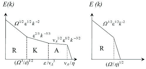
		$k$	$k$
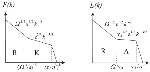
	$k$		$k$

Figure 1: Possible inertial regimes of energy spectral density in rotating MHD turbulence for $\mathrm{Pm}=1$. The capital letters $R,A$ and $K$ denote a rotating, Alfvén or Kolmogorov turbulence.

The four possible types of inertial regimes are sketched in Fig. 1 in which the spectral energy density is plotted versus $k$ for $\mathrm{Pm}=1$. The slopes and characteristic wave numbers are indicated. The conditions to get one of these four possible inertial regimes are summarized in the plane $(V_{A},\Omega)$ in Fig. 2. The case without rotation corresponds to the abscissa axis. Then two regimes KA or K are possible depending whether $\eta/V_{A}^{2}\leq V_{A}^{2}/\varepsilon$ or not. The case without applied magnetic field corresponds to the vertical axis. Then the two regimes R or RK are possible depending whether $\eta\Omega/\varepsilon\geq\Omega^{-1}$ or not. Without both rotation and applied magnetic field a K type of turbulence is found.

From our analysis we note that inertial regimes of type AK or RAK are never possible. On the other hand inertial regimes of type KA, A, or K are possible provided the forcing scale is sufficiently small. In Fig. 1 it corresponds to begin the spectra at a larger wave number. For $\mathrm{Pm}<1$ the inertial range of the kinetic energy spectrum prolongates at scales smaller than $k_{\eta}$ with either an R, K or RK spectrum.

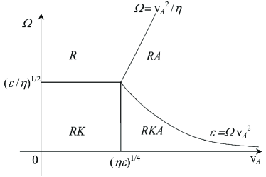
Figure 2: The four possible turbulent inertial regimes given in the map $(V_{A},\Omega)$.

III Shell model

III.1 The model

The equations of MHD turbulence for an incompressible fluid embedded in an external uniform magnetic field $\boldsymbol{\rm B}_{0}$ and subject to rotation $\boldsymbol{\Omega}$ write

$$\partial\boldsymbol{\rm u}/\partial t + (\boldsymbol{\rm u}\cdot\nabla)\boldsymbol{\rm u}-((\boldsymbol{\rm B}+\boldsymbol{\rm v}_{A})\cdot\nabla)\boldsymbol{\rm B}+2\boldsymbol{\Omega}\times\boldsymbol{\rm u}$$ (7)

$$= \nu\nabla^{2}\boldsymbol{\rm u}+\boldsymbol{\rm F}-\nabla P_{t}$$

$$\partial\boldsymbol{\rm B}/\partial t + (\boldsymbol{\rm u}\cdot\nabla)\boldsymbol{\rm B}-((\boldsymbol{\rm B}+\boldsymbol{\rm v}_{A})\cdot\nabla)\boldsymbol{\rm u}=\eta\nabla^{2}\boldsymbol{\rm B}$$ (8)

$$\nabla\cdot\boldsymbol{\rm u} = \nabla\cdot\boldsymbol{\rm B}=0$$ (9)

in which $\textbf{v}_{A}=\boldsymbol{\rm B}_{0}/\sqrt{\mu\rho}$ is the Alfvén velocity (where $\mu$ and $\rho$ are respectively the fluid magnetic permeability and density) and $\boldsymbol{\rm B}$ is given in unit of $V_{A}=|\boldsymbol{\rm v}_{A}|$. The total pressure $P_{t}=P+b^{2}/2$ is a functional of $\boldsymbol{\rm u}$ and $\boldsymbol{\rm B}$ owing to the incompressibility condition (9). The forcing $\boldsymbol{\rm F}$ insures the fluid motion.

From (7) (8) (9) we derive the following shell model

$$\dot{U}_{n} = ik_{n}\left[Q_{n}(U,U)-Q_{n}(B,B)\right]$$ (10)

$$+ ik_{n}V_{A}(t)B_{n}+i\Omega(t)U_{n}-\nu k_{n}^{2}U_{n}+F_{n}(t),$$

$$\dot{B}_{n} = ik_{n}\left[Q_{n}(U,B)-Q_{n}(B,U)\right]$$ (11)

$$+ ik_{n}V_{A}(t)U_{n}-\eta k_{n}^{2}B_{n},$$

where

$$Q_{n}(X,Y)=\lambda^{2}(X_{n+1}Y_{n+1}+X_{n+1}^{*}Y_{n+1}^{*})-X_{n-1}^{r}Y_{n}$$

$$-X_{n}Y_{n-1}^{r}+{\rm i}\lambda(2X_{n}^{*}Y_{n-1}^{i}+X_{n+1}^{r}Y_{n+1}^{i}-X_{n+1}^{i}Y_{n+1}^{r})$$

$$+X_{n-1}Y_{n-1}+X_{n-1}^{*}Y_{n-1}^{*}-\lambda^{2}(X_{n+1}^{r}Y_{n}+X_{n}Y_{n+1}^{r})$$

$$+{\rm i}\lambda(2X_{n}^{*}Y_{n+1}^{i}+X_{n-1}^{r}Y_{n-1}^{i}-X_{n-1}^{i}Y_{n-1}^{r}),$$ (12)

represents the non linear transfer rates and $F_{n}$ the turbulence forcing. This model is based on wavelet decompostion Zimin and Hussain (1995). Compared to other shell models Gledzer (1973); Ohkitani and Yamada (1989); L’vov et al. (1998) it has the advantage that helicities are much better defined, like those based on helical wave decomposition Benzi et al. (1996); Lessines et al. (2009); Lessines and Carati (2009). It has been introduced in its hydrodynamic form to study spectral properties of helical turbulence Stepanov et al. (2009), and in its MHD form to study cross-helicity effect on cascades Mizeva et al. (2009). The parameter $\lambda$ is the geometrical factor from which the wave number is defined $k_{n}=k_{0}\lambda^{n}$. As explained in Plunian and Stepanov (2007) an optimum shell spacing is the golden number $\lambda=(1+\sqrt{5})/2$. The terms involving $\Omega$ and $V_{A}$ were already introduced in several previous papers dealing with either rotation Hattori et al. (2004); Chakraborty et al. (2010) or applied magnetic field Biskamp (1994); Hattori and Ishizawa (2001).

III.2 Conservative quantities

Expressions for the kinetic energy and helicity, $E_{U}$ and $H_{U}$, magnetic energy and helicity, $E_{B}$ and $H_{B}$, and cross helicity $H_{C}$, are given by

$$E_{U} = \sum_{n}E_{U}(n),\;E_{U}(n)=\frac{1}{2}|U_{n}|^{2},$$ (13)

$$H_{U} = \sum_{n}H_{U}(n),\;H_{U}(n)=\frac{i}{2}k_{n}((U_{n}^{*})^{2}-U_{n}^{2}),$$ (14)

$$E_{B} = \sum_{n}E_{B}(n),\;E_{B}(n)=\frac{1}{2}|B_{n}|^{2},$$ (15)

$$H_{B} = \sum_{n}H_{B}(n),\;H_{B}(n)=\frac{i}{2}k_{n}^{-1}((B_{n}^{*})^{2}-B_{n}^{2}),$$ (16)

$$H_{C} = \sum_{n}H_{C}(n),\;H_{C}(n)=\frac{1}{2}(U_{n}B_{n}^{*}+B_{n}U_{n}^{*}).$$ (17)

In the inviscid and non-resistive limit ($\nu=\eta=0$), the total energy $E=E_{U}+E_{B}$, magnetic helicity and cross helicity must be conserved ($\dot{E}=\dot{H}_{B}=\dot{H}_{C}=0$). Here with the additional Coriolis and Alfvénic terms the properties of conservation are not necessarily satisfied. A summary of theses properties is given in table 1 for 3D MHD turbulence. In the case of pure hydrodynamic turbulence (without magnetic field) the kinetic energy and helicity must be conserved ($\dot{E_{U}}=\dot{H}_{U}=0$) even with Coriolis forces.

$\Omega$	=0	$\neq 0$	$=0$	$\neq 0$
$V_{A}$	=0	$=0$	$\neq 0$	$\neq 0$
$E$	Y	Y	Y	Y
$H_{C}$	Y	N	Y	N
$H_{M}$	Y	Y	N	N

Table 1: In 3D MHD turbulence, conservation properties of total energy $E$, cross-helicity $H_{C}$ and magnetic helicity $H_{M}$ depending on global rotation $\Omega$ and applied field $V_{A}$.

III.3 Time-scales

In (10) and (11) the forcing $F_{n_{F}}(t)$ (applied at some scale $k_{n_{F}}^{-1}$), the global rotation $\Omega(t)$ and the applied field $V_{A}(t)$ have constant intensities $|F_{n_{F}}|,\Omega$ and $V_{A}$. Only their sign may change after a period of time $t_{F}$, $t_{\Omega}$ and $t_{V_{A}}$, the probability of changing from one period to the next being random. Such a trick allows to control the two characteristic times $\tau_{\Omega}\approx t_{\Omega}$ and $\tau_{V_{A}}\approx t_{V_{A}}$. In the simulations we take $t_{\Omega}=1/\Omega$ and $t_{V_{A}}=1/(k_{n_{F}}V_{A})$. It is in same spirit than the one used in Hattori and Ishizawa (2001) and Hattori et al. (2004) though much simpler. Incidentally the random change of sign of $\Omega(t)$ insures that there is no injection of kinetic helicity on average. Taking a random sign in $F_{n_{F}}(t)$ we insure that the forcing intensity satisfies $|F_{n_{F}}|\approx\sqrt{2\varepsilon/t_{F}}$. It is also important that $t_{F}$ is the shortest among all other characteristic times of the problem $\tau_{K},\tau_{\Omega}$ and $\tau_{V_{A}}$ (and of course $\tau_{\eta}$). We choose $t_{F}\leq\frac{1}{10}\min\left\{\tau_{K},\tau_{\Omega},\tau_{V_{A}}\right\}$.

III.4 No injection of cross-helicity

In addition it is important to control the injection of cross-helicity as was shown in Mizeva et al. (2009). Indeed any spurious injection of cross-helicity may lead to a supercorrelation state where $U_{n}\approx B_{n}$ implying equality not only in intensity (as in equipartition) but also in phase. In that case the flux of kinetic energy is depleted, implying an accumulation of energy at large scale and steeper spectral slopes. In order to compare the results to the phenomenological approach we impose the injection of cross-helicity to be zero. For that we could use the forcing

$$\frac{F_{n_{F}}}{|F_{n_{F}}|}=\pm i\frac{B_{n_{F}}}{|B_{n_{F}}|}$$ (18)

where again the sign is randomly changed after each period of time $t_{F}$. This forcing is however ill-defined as soon as $|B_{n_{F}}|\ll|U_{n_{F}}|\approx 1$. To fix this problem we use the following forcing

$$\frac{F_{n_{F}}}{|F_{n_{F}}|}=\frac{ae^{i\varphi}\pm i\zeta\frac{B_{n_{F}}}{|B_{n_{F}}|}}{a+\zeta}$$ (19)

with $\zeta=|B^{2}_{n_{F}}|/|U^{2}_{n_{F}}|$, in which $\varphi$ is a phase randomly changed after each period of time $t_{F}$, and $a$ an additional parameter. In the case $\zeta\gg a$, (18) is recovered, and the phase of $F_{n_{F}}$ is mainly determined by the phase of $B_{n_{F}}$ so that it corresponds to zero injection of cross-helicity. In the case $\zeta\ll a$ the phase of $F_{n_{F}}$ is controlled by the random phase $\varphi$. Since $B_{n_{F}}$ is small there is no cross-helicity injection too. The value $a=10^{-6}$ provides a robust forcing with always a low level of cross-helicity.

III.5 Dissipations

We define the dissipation of $U$ and $B$ at scale $k_{n}$ by $D_{U}(k_{n})=\nu k_{n}^{2}|U_{n}|^{2}$ and $D_{B}(k_{n})=\eta k_{n}^{2}|B_{n}|^{2}$. From the phenomenological formalism above we expect the total dissipation to be equal to the injection rate of energy at the forcing scale $\varepsilon_{\nu}+\varepsilon_{\eta}=\varepsilon$, with $\varepsilon_{\nu}=\sum_{n}D_{U}(k_{n})$ and $\varepsilon_{\eta}=\sum_{n}D_{B}(k_{n})$. Equivalently in pure HD we would have $\varepsilon_{\nu}=\varepsilon$. On the other hand the ratio of both dissipations $\rho=\varepsilon_{\eta}/\varepsilon_{\nu}$ cannot be predicted. It can only be calculated numerically.

IV Results

IV.1 Spectra for $\mathrm{Pm}=1$

$\quad\quad\quad\quad\Omega^{-1/2}\varepsilon^{-1/2}k^{2}E(k)$
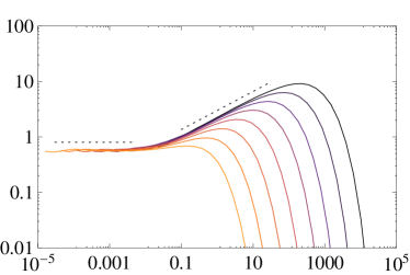
	$\Omega^{-3/2}\varepsilon^{1/2}k$
$\varepsilon^{-2/3}k^{5/3}E(k)$
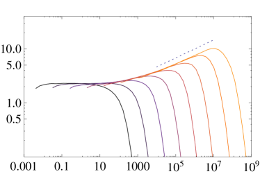
	$V_{A}^{3}\varepsilon^{-1}k$
$k^{3/2}\varepsilon^{-1/2}V_{A}^{-1/2}E(k)$
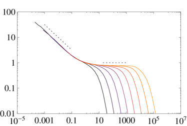
	$V_{A}\Omega^{-1}k$

Figure 3: (Color online) Normalized spectra for $\nu=10^{-7}$ and $\mathrm{Pm}=1$. Curves (a) are shown for $V_{A}=0$ and $\Omega=12.5,25,50,10,200,400,800,1600$ (from right to left, from darker to lighter). Curves (b) are shown for $\Omega=0$ and $V_{A}=0.16,0.32,0.64,1.28,2.56,5.12,10.24,20.48$ (from left to right, from darker to lighter). Curves (c) are shown for $(V_{A},\Omega)=(0.16,800);(0.32,400);(0.64,200);(1.28,100);(2.56,50);$ $(5.12,25);(10.24,12.5);(20.48,6.25)$ (from left to right, from darker to lighter).

In Fig. 3 the spectra are plotted for $\nu=10^{-7}$ and $\mathrm{Pm}=1$ in the three cases $V_{A}=0$, $\Omega=0$, and $V_{A}\Omega\neq 0$. For $V_{A}=0$, the horizontal and $k^{1/3}$ dashed lines disclose a RK regime. For $\Omega=0$, the dashed line $k^{1/6}$ disclose a KA regime. For $V_{A}\Omega\neq 0$, the $k^{-1/2}$ and horizontal dashed lines disclose a RA regime. In each case the transition between two power laws is rather smooth and occurs over a scales range of about two orders of magnitude.

For $\varepsilon\approx 1$ and taking the numerical values for $\Omega,V_{A}$ and $\eta$ given in Fig. 2 we find that the three sets of spectra found with the shell model belong indeed to the three parts RK, (R)KA and RA of Fig. 2. We tried to track the transition from one part to the other, varying $\Omega$ and $V_{A}$. It is however not possible to handle it numerically as the spectral slopes are not so well defined at the neighborhood of the frontiers delimiting the four parts of Fig. 2.

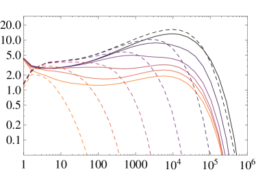
$k^{2}E(k)\varepsilon^{-1/2}$		$k^{2}E(k)\varepsilon^{-1/2}$
	$k\varepsilon^{1/2}$		$k\varepsilon^{1/2}$
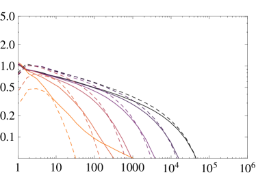
$k^{5/3}E(k)\varepsilon^{-2/3}$		$k^{3/2}E(k)\varepsilon^{-1/2}$
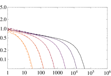
	$k\varepsilon^{-1}$		$k\varepsilon^{-1}$
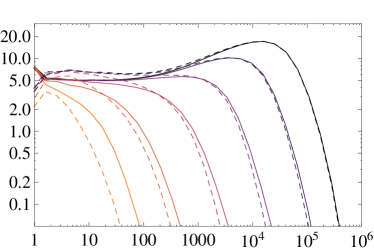
$k^{2}E(k)\varepsilon^{-1/2}$		$k^{3/2}E(k)\varepsilon^{-1/2}$
	$k\varepsilon^{-1}$		$k\varepsilon^{-1}$

Figure 4: (Color online) Normalized kinetic (full) and magnetic (dashed) spectra for $\nu=10^{-7}$: (a) $(V_{A},\Omega)=(0,100)$, (b) $(V_{A},\Omega)=(0,1600)$. (c) $(V_{A},\Omega)=(0.08,0)$, (d) $(V_{A},\Omega)=(1.28,0)$. (e) $(V_{A},\Omega)=(0.32,400)$, (f) $(V_{A},\Omega)=(20.48,6.25)$. For each set of curves for $\mathrm{Pm}=10^{-5},10^{-4},10^{-3},10^{-2},10^{-1},1$ (from lighter to darker). Note, that the kinetic and magnetic spectra are superposed in the case (f).

IV.2 Spectra for $\mathrm{Pm}<1$

In Fig. 4 the kinetic and magnetic spectra are plotted for $\nu=10^{-7}$ and several values of $\mathrm{Pm}$, for the three previous cases.

For $V_{A}=0$ (a,b) increasing $\mathrm{Pm}$ decreases the magnetic dissipation scale while the viscous scale is not significantly changed. This is in agreement with a simple Kolmogorov phenomenology Stepanov and Plunian (2008), the ratio of dissipation scales being given by $k_{\nu}/k_{\eta}\propto\mathrm{Pm}^{-3/4}$. For $\mathrm{Pm}\geq 10^{-2}$ the effect of rotation is visible in the spectra flatness. At smaller values of $\mathrm{Pm}$ it is however difficult to determine any slope at all.

For $\Omega=0$ and $V_{A}=1.28$ (c,d) both kinetic and magnetic spectra are almost the same whatever the value of $\mathrm{Pm}$. The effect of an applied magnetic field is to correlate both fields as expected in Alfvén waves. In particular the dissipation scale is governed by the magnetic diffusivity, with $k_{\nu}\approx k_{\eta}$ . The same conclusions are found for $(V_{A},\Omega)=(0.32,400)$ (e) and $(V_{A},\Omega)=(20.48,6.25)$ (f). In these two cases the horizontal slopes are due to rotation (e) and applied magnetic field (f).

We note that for $\Omega=0$ and $V_{A}=1.28$ (d) the normalized curves are not horizontal. They correspond to spectral energy density slopes between $k^{-5/3}$ and $k^{-3/2}$. The latter is obtained for values of $V_{A}$ about ten times larger.

Figure 5: Dissipation ratio versus $\mathrm{Pm}$. On panel (a) $V_{A}=\Omega=0$ and the full curves from right to left correspond to $\nu=10^{-5}$, $10^{-6}$, $10^{-7}$, $10^{-8}$. The dashed curves from bottom to top correspond to $\eta=1/4$, $1/8$, $1/16$, $1/32$, $1/64$, $1/128$, $1/256$. On panel (b) $V_{A}=0$, $\nu=10^{-7}$ and the curves correspond to $\Omega=0$ (full curve), $100$ (dashed), $400$ (dotted), 1600 (dot-dashed). On panel (c) $\Omega=0$, $\nu=10^{-7}$ and the curves correspond to $V_{A}=0$ (full curve), $0.08$ (dashed), $0.32$ (dotted), 1.28 (dot-dashed). On panel (d) $\nu=10^{-7}$ and the curves from bottom to top correspond to $(V_{A},\Omega)=(0,0)$, (0.32, 400), (2.56,50) and (20.48,6.25).

IV.3 Dissipation ratio

In Fig. 5 the ratio $\rho=\varepsilon_{\eta}/\varepsilon_{\nu}$ is plotted versus $\mathrm{Pm}$ for $V_{A}=\Omega=0$ (a), $V_{A}=0$ (b), $\Omega=0$ (c) and $V_{A}\Omega\neq 0$ (d). In the limit $\mathrm{Pm}\rightarrow 0$ the dynamo action does not occur, implying $\rho\rightarrow 0$. For $\mathrm{Pm}=1$ both kinetic and magnetic spectra are identical, implying $\varepsilon_{\nu}=\varepsilon_{\eta}=\varepsilon/2$, and then $\rho=1$. We always find an intermediate value of $\mathrm{Pm}$ for which $\rho$ reaches a maximum. This is related to a super-equipartition state in which the magnetic energy is higher than the kinetic energy at large scales. Varying $V_{A}$ and $\Omega$ we find that this maximum value can increase by several orders of magnitude and that it does not occur at the same $\mathrm{Pm}$. For the two last cases an asymptotic curve $\rho=O(\mathrm{Pm}^{-1})$ is obtained for large values of $V_{A}$. This is a direct consequence of the equipartition regime $|U_{n}|\approx|B_{n}|$ obtained at any scale (see Fig. 4). In that cases the definition of $\rho$ directly implies the scaling $O(\mathrm{Pm}^{-1})$.

V Discussion

For $\mathrm{Pm}=1$ both approaches, phenomenological and shell model, give consistent results in terms of inertia regimes. They are controlled by the shortest time-scale corresponding either to rotation, applied magnetic field, inertia, or a combination of them. For $\mathrm{Pm}<1$ the magnetic dissipation occurs at a scale larger than the viscous scale implying that the different regimes are not so easy to discriminate. However for a sufficiently strong applied magnetic field both kinetic and magnetic energy spectra are merged, implying a strong increase of the viscous dissipation scale. Whether this is due to our isotropic assumption is not clear and cannot be answered with our models. A consequence is that, for a strong applied field, the ratio of magnetic to kinetic dissipation scales like $O(\mathrm{Pm}^{-1})$ and can reach very high values for $\mathrm{Pm}\ll 1$. Without applied field, this ratio is also maximum for some value of $\mathrm{Pm}\ll 1$, depending on the fluid viscosity and global rotation.