Casimir force in the presence of a medium

Abstract

In this article we investigate the Casimir effect in the presence of a medium by quantizing the Electromagnetic (EM) field in the presence of a magnetodielectric medium by using the path integral formalism. For a given medium with definite electric and magnetic susceptibilities, explicit expressions for the Casimir force are obtained which are in agree with the original Casimir force between two conducting parallel plates immersed in the quantum electromagnetic vacuum.

I introduction

One of the most remarkable and fundamentally important result of the field quantization is the Casimir effect which is a force arising from the change of the zero point energy caused by imposing the boundary conditions (BC) Casimir . This force is the macroscopic aspect of the quantum electrodynamics that provides a direct line between quantum field theory and the macroscopic world. The original calculation of the Casimir force between two perfectly conducting parallel plates immersed in the quantum electromagnetic vacuum is based on the definition of the Casimir energy in the presence and the absence of boundary surfaces Casimir that leads to an attractive observable force

$$F=-\frac{\hbar c}{240}\frac{1}{H^{4}},$$ (1)

between the plates, where $\hbar$ is the Planck constant, $c$ is the speed of light and $H$ is the distance between the plates. In other way one can consider this effect by evaluating the radiation pressure on macroscopic objects Milonni . As the magnitude of the Casimir force is substantial at $H<100~{}{\text{nm}}$ this effect is relevant in nano-technology sriva ; nanoscale1 ; nanoscale1b ; s2 and should be take into account to design and actuate microelectromechanical (MEMS) systems. Moreover the possibility of transducing the energy from the vacuum is investigated by means of MEMS pinto ; Cole ; Forward .

Many attempts have been focused on observing the Casimir force and performing high-precision measurements during last few years Lamoreaux ; Mohideen ; Harris ; Bressi ; Decca1 ; Decca2 . All these experiments are in agree with the prediction of the Casimir Casimir within a few percents. These deviation from the ideal force may due to temperature, roughness of surfaces and finite dielectric constants that have been covered in a very recent book entitled by Advanced in the Casimir Effect Bordag_Book .

In 90th decade, Golestanian and Kardar developed a path integral approach to investigate the dynamic Casimir effect in the system of two corrugated conducting plates surrounded by the quantum vacuum Golestanian-PRL-1997 ; Golestanian-PRA-1998 . Emig and his colleagues also used the path integral formalism to obtain normal and lateral Casimir force between two sinusoidal corrugated perfect conductor surfaces Emig-PRL-2001 ; Emig-PRA-2003 . Later on, the exact mechanical response of the quantum vacuum to the dynamic deformations of a cavity and the rate of dissipation have been calculated by using path integral scheme jalal . This motivated us to investigate the Casimir effect in the presence of a magnetodielectric medium by quantizing the electromagnetic (EM) field using path integral formalism. Our system contains of a magnetodielectric medium with permitivity $\varepsilon$ and permeability $\mu$, enclosed by two semi-infinite ideal metals ($\varepsilon_{\text{L}}\rightarrow\infty$ for the ideal metal in left-hand side and $\varepsilon_{\text{R}}\rightarrow\infty$ for right-hand side one) as depicted in Fig. ​(1). We model the magnetodielectric medium by a continuum of harmonic oscillators (Hopfield Model) Fardin1 ; Fardin2 ; Fardin3 .

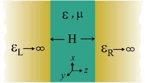
Figure 1: This picture illustrates the schematic figure of the system under consideration. A magnetodielectric medium ($\varepsilon,~{}\!\mu$) is enclosed between two perfect parallel conductors ($\varepsilon_{\text{R}}$ and $\varepsilon_{\text{L}}\rightarrow\infty$). The distance between conductors is $H$, and the $z$ direction is perpendicular to the surfaces of the media.

The outline of this paper is as follows: In Sec. II, in order to introduce the scheme, we first quantize the simple case of a scaler Klein-Gordon field in the presence of a medium. Sec. III is devoted to obtain the Casimir force for the scalar filed in the presence of a medium for different kinds of boundary conditions. In Sec. IV, we develop our formalism to the case of EM field in the presence of a magnetodielectric medium. Sec. V gives the Casimir force for the case of EM field. Finally, the conclusions and outlooks are in the Sec. VI.

II Field quantization using path integrals

To illustrate the method and also for later convenience, before considering the EM field in the presence of a medium, we consider the simplest case i.e. a scaler massless field. In the next section we will show that the Klein-Gordon field can be corresponded to each polarization of the EM field. Therefore, let us consider the following Lagrangian for the total system

$${\cal{L}}={\cal{L}}_{sys}+{\cal{L}}_{mat}+{\cal{L}}_{int},$$ (2)

where

$${\cal{L}}_{sys}=\frac{1}{2}\,\partial^{\mu}\varphi\,\partial_{\mu}\varphi,$$ (3)

is the Lagrangian density of the massless Klein$-$Gordon filed. The medium is modeled by a continuum of harmonic oscillators as Huttner

$${\cal{L}}_{mat}=\int_{0}^{\infty}d\omega\,(\frac{1}{2}\rho\dot{Y}_{\omega}^{2}-\frac{1}{2}\rho\omega^{2}Y_{\omega}^{2}),$$ (4)

where $Y_{\omega}$ is an oscillator’s field, $\rho$ is the density of matter field and the interaction between the system and its medium is defined by

$${\cal{L}}_{int}=\varphi\dot{P},$$ (5)

where

$$P=\int d\omega\nu(\omega)Y_{\omega}.$$ (6)

In the next section we will show that the quantity $P$ is in fact the polarization field corresponding to the medium and the interaction (5) will become the electric-dipole interaction.

Generally a generating function is defined by Ryder

$$Z[J]=\int{\cal{D}}[\psi]\exp{\bigg{\{}\imath\int d^{n+1}x[{\cal L}\big{(}\psi(x)\big{)}+J(x)\psi(x)]\bigg{\}}},$$ (7)

where $\psi$ is the scalar field and the different correlation functions can be found by taking the repeated functional derivatives with respect to the source field $J(x)$. The above partition function is Gaussian since the integrand has quadratic form with respect to the fields. To obtain the generating function for the interacting fields, we first calculate the generating function for the free fields

$$Z_{0}\!\! \!\![J_{\varphi},J_{\omega}]=\int{\cal{D}}[\varphi]\prod_{\omega}{\cal{D}}[Y_{\omega}]\times$$

$$\times\exp\bigg{\{}\imath\int d^{n+1}x\big{[}{\cal{L}}_{sys}+{\cal{L}}_{mat}+J_{\varphi}\varphi+\int d\omega J_{\omega}Y_{\omega}\big{]}\bigg{\}}.$$

Using the $n$-dimensional version of Gauss’s theorem we find

$$\int d^{n+1}x\,\partial_{\mu}\varphi\,\partial^{\mu}\varphi=-\int d^{n+1}x\,\varphi\,\Box\,\varphi,$$ (9)

where $\Box$ is the d’Alemberian in $(n+1)$-dimensional space-time and the integration by part

$$\int d^{n+1}x\,\,\dot{Y}_{\omega}\,\dot{Y}_{\omega}=-\int d^{n+1}x\,Y_{\omega}\,\frac{{\partial^{2}}}{{\partial t^{2}}}\,Y_{\omega}.$$ (10)

the free generating function (II) can be written as

$$Z_{0}\!\! \!\![J_{\phi},J_{\omega}]=\int\prod_{\omega}{\cal D}[Y_{\omega}]{\cal D}[\varphi]\exp\bigg{\{}-\frac{\imath}{2}\int d^{n+1}x$$ (11)

$$\times\bigg{[}\varphi(x)\Box\varphi(x)+\int d\omega Y_{\omega}(x)(\frac{{\partial^{2}}}{{\partial t^{2}}}+\rho\omega^{2})Y_{\omega}(x)$$

$$~{}~{}~{}+J_{\varphi}(x)\varphi(x)+\int d\omega J_{\omega}(x)Y_{\omega}(x)\bigg{]}\bigg{\}}.$$

The integral in the equation (11) can be easily calculated from the field version of the quadratic integrals and the result is

$$Z_{0}\!\! \!\![J_{\varphi},J_{\omega}]=$$ (12)

$$\!\!\!\!\!\!\!=\exp\bigg{\{}-\frac{\imath}{2}\int d^{n+1}x\int d^{n+1}x^{\prime}\!\bigg{[}J_{\varphi}(x)G_{0}(x-x^{\prime})J_{\varphi}(x^{\prime})$$

$$\hskip 25.6073pt+\int\!\!d\omega J_{\omega}(x)G_{\omega}(x-x^{\prime})J_{\omega}(x^{\prime})\bigg{]}\!\bigg{\}},$$

where $G_{\omega}(x-x^{\prime})$ and $G_{0}(x-x^{\prime})$ are the propagators for free fields and satisfy the following equations

$$\Box G_{0}(x-x^{\prime})=\delta(x-x^{\prime}),$$ (13)

$$\{\rho\frac{{\partial^{2}}}{{\partial t^{2}}}+\rho\omega^{2}\}G_{\omega}(x-x^{\prime})=\delta(x-x^{\prime}).$$ (14)

We employ the Fourier transformation to solve the equations (13) and (14). The solutions are

$$G_{0}(x-x^{\prime})=\frac{1}{(2\pi)^{n+1}}\int d^{n}{\bf k}\,d\omega\,\frac{{e^{\imath{\bf k}\cdot({\bf x}-{\bf x}^{\prime})-\imath\omega(t-t^{\prime})}}}{{\omega^{2}-{\bf k}^{2}}},$$ (15)

and

$$G_{\omega}(x-x^{\prime})=\frac{1}{(2\pi\rho)}\int d\omega^{\prime}\,\frac{{e^{-\imath\omega^{\prime}(t-t^{\prime})}}}{{\omega^{2}-\omega^{\prime 2}}}\,\delta({\bf x}-{\bf x^{\prime}}).$$ (16)

Here the space component of the point $x\in{\cal R}^{n+1}$ is indicated by the bold face ${\bf{x}}\in{\cal R}^{n}$ and the time component by $t$ or $x_{0}\in{\cal R}$.

For further use we define

$$J_{p}(z)=\int d\omega\nu(\omega)J_{\omega}(z),$$ (17)

the generating function of the interacting fields can be written in terms of the free generating function as Ryder

$$Z[J_{\varphi},J_{P}] = Z^{-1}[0]e^{\imath\int d^{n+1}z{\cal{L}}_{int}(\frac{\delta}{\delta J_{\varphi}(z)},\frac{\delta}{\delta J_{P}(z)})}Z_{0}[J_{\varphi},J_{\omega}]$$ (18)

$$=Z^{-1}[0]\sum\limits_{n=0}^{\infty}\frac{1}{n!}\bigg{[}\imath\int d^{n+1}z\frac{\delta}{{\delta J_{\varphi}(z)}}\cdot\frac{\partial}{{\partial z_{0}}}\frac{\delta}{{\delta J_{\varphi}(z)}}\bigg{]}^{n}\times$$

$$\hskip 17.07182pt\times Z_{0}[J_{\varphi},J_{\omega}],$$

where $Z[0]$ is the partition function of the free space. Thus the Green’s function of Klein-Gordon filed can be obtained via

$$G_{\varphi\varphi}(x-y)=\imath\frac{{\delta^{2}Z[J_{\varphi},J_{P}]}}{{\delta J_{\varphi}(x)\delta J_{\varphi}(y)}}\big{|}_{J_{\varphi},J_{\omega}=0}.$$ (19)

Combining the generating function (18), the Green’s function (19) and the definition of ${\cal L}_{int}$ (5) yield the following series for the Green’s function

$$G_{\varphi\varphi}(x-x^{\prime}) = G_{0}(x-x^{\prime})$$ (20)

$$+\!\!\int\!\!d\omega\!\!\int\!\!dx_{1}dx_{2}G_{0}(x\!-\!x_{1}\!)\nu^{2}(\omega)\frac{{\partial^{2}}}{{\partial t^{2}}}G_{\omega}(x_{1}\!-\!x_{2}\!)G_{0}(x_{2}\!-\!x^{\prime})$$

$$+\!\!\!\int\!\!\!d\omega\!\!\!\int\!\!\!d\omega^{\prime}\!\!\!\!\int\!\!\!dx_{1}dx_{2}\!\!\!\int\!\!\!dx_{3}dx_{4}G_{0}(x\!-\!x_{1}\!)\nu^{2}(\omega)\frac{{\partial^{2}}}{{\partial t^{2}}}G_{\omega}(x_{1}\!\!-\!x_{2}\!)\!\!\times$$

$$\times G_{0}(x_{2}\!-\!x_{3}\!)\nu^{2}(\omega^{\prime})\frac{{\partial^{2}}}{{\partial t^{2}}}G_{\omega^{\prime}}(x_{3}\!-\!x_{4}\!)G_{0}(x_{4}\!-\!x^{\prime})\!+\!\cdots.$$

It is appropriate to use a general Green’s function in $(n+1)$-dimensional Fourier space that is

$$G({\bf k},\omega)=\int e^{\imath{\bf k}\cdot{\bf x}-\imath\omega t}\,G(x)\,dt\,d^{n}\,{\bf x}.$$ (21)

Therefore the Green’s functions of the free fields $\varphi$ and $Y_{\omega}$ in the Fourier space might be given by

$$G_{0}({\bf k},\omega)=\frac{1}{{{\bf k}^{2}-\omega^{2}}},$$ (22)

and

$$G_{\omega}({\bf k},\omega^{\prime}) = \frac{1}{\rho}\int\frac{d\omega^{\prime\prime}dt\,d^{3}{\bf x}~{}{e^{-\imath\omega^{\prime\prime}t}}}{{\omega^{2}-\omega^{{}^{\prime\prime}2}-\imath 0^{+}}}\delta({\bf x})e^{\imath(\omega^{\prime}t-{\bf k}\cdot{\bf x})}$$ (23)

$$= \frac{1}{\rho}\frac{1}{\omega^{2}-\omega^{{}^{\prime}2}-\imath 0^{+}}=:G_{\omega}(\omega^{\prime}),$$

respectively. Since we are interested in retarded Green’s functions we have added $-\imath 0^{+}$ to the denominator of the equation (23). Since the reservoir field is assumed to be homogeneous, the Green’s function of the reservoir does not depend on ${\bf k}$ in the above equation. Using the equations (22) and (23), $G_{\varphi\varphi}(x-x^{\prime})$ can be written in the Fourier space as

$$G_{\varphi,\varphi}({\bf k},\omega)$$ (24)

$$=G_{0}({\bf k},\omega)\{1+\sum\limits_{n=0}^{\infty}[\int d\omega^{\prime}\omega^{2}\nu^{2}(\omega^{\prime})G_{\omega^{\prime}}(\omega)G_{0}({\bf k},\omega)]^{n}\}$$

$$=\frac{G_{0}({\bf k},\omega)}{1-\int d\omega^{\prime}\omega^{2}\nu^{2}(\omega^{\prime})G_{\omega^{\prime}}(\omega)G_{0}({\bf k},\omega)}$$

$$=\frac{1}{{{\bf k}^{2}-\omega^{2}-\frac{1}{\rho}\int d\omega^{\prime}\frac{\nu^{2}(\omega^{\prime})\omega^{2}}{\omega^{\prime 2}-\omega^{2}+\imath 0^{+}}}}.$$

This Green’s function can also be obtained directly from the Heisenberg equations of motion. By direct substitution we can show that the Green’s function $G_{\varphi\varphi}(x-y)$ satisfies the equation

$$\!\!\!\!\!\Box G_{\varphi\varphi}({\bf x}-{\bf x}^{\prime},t-t^{\prime})$$

$$\!\!\!\!\!-\frac{\partial}{{\partial t}}\!\!\int_{-\infty}^{t}\!\!\!\!\!dt^{\prime\prime}\!\chi(t\!-\!t^{\prime\prime})\frac{\partial}{{\partial t^{\prime\prime}}}G_{\varphi\varphi}({\bf x}\!-\!{\bf x}^{\prime},t^{\prime\prime}\!\!-\!t^{\prime})\!=\!\delta({\bf x}\!-\!{\bf x}^{\prime},t\!-\!t^{\prime}),$$

which is the motion equation of dissipation field with susceptibility of the medium $\chi(t)$, with the following Fourier transform

$$\chi(\omega)=\frac{1}{\rho}\int d\omega^{\prime}\frac{{\nu^{2}(\omega^{\prime})}}{{\omega^{{}^{\prime}2}-\omega^{2}+\imath 0^{+}}}.$$ (26)

From the equations (24) and (26) it is clear that the modified Green’s function $G_{\varphi,\varphi}({\bf k},\omega)$ can be obtained from the free field Green’s function $G_{0}(x-x^{\prime})$ in Eq. ​(15) simply by replacing $\omega^{2}$ with $\varepsilon(\omega)\omega^{2}$, where $\varepsilon(\omega):=1+\tilde{\chi}(\omega)$. It can be easily shown that this susceptibility satisfies the Kramers-Kronig relations as expected.

By the same technique we can obtain correlation between the polarization field and the Klein-Gordon field. To this end we define $G_{\varphi,P}$ as

$$G_{\varphi,P}=\frac{\delta^{2}Z[J_{\varphi},J_{P}]}{\delta J_{\varphi}\delta J_{P}},$$ (27)

that can be obtained via direct calculation similar to the procedure that ended to $G_{\varphi,\varphi}({\bf k},\omega)$ as

$$G_{\varphi,P}(x-x^{\prime})=\int dx_{1}G_{0}(x-x_{1})\frac{\partial}{\partial z_{0}}G_{0P}(x_{1}-x^{\prime})$$

$$+\int dx_{1}dx_{2}G_{0P}(x-x_{1})\frac{{\partial^{2}}}{{\partial t^{2}}}G_{0}(x_{1}-x_{2})G_{0P}(x_{2}-x^{\prime})$$

$$+\int dx_{1}dx_{2}\int dx_{3}dx_{4}G_{0P}(x-x_{1})\frac{{\partial^{2}}}{{\partial t^{2}}}G_{0}(x_{1}-x_{2})\times$$

$$\times G_{0P}(x_{2}-x_{3})\frac{{\partial^{2}}}{{\partial t^{2}}}G_{0}(x_{3}\!-\!x_{4})G_{0P}(x_{4}\!-\!x^{\prime})+\cdots,$$ (28)

where

$$G_{0P}(x-x^{\prime})=\int d\omega\nu^{2}(\omega)G_{\omega}(x-x^{\prime}).$$ (29)

If we again write $G_{\varphi,P}(x-x^{\prime})$ in the Fourier space we find

$$G_{\varphi,P}({\bf k},\omega) = \imath\omega G_{0}({\bf k},\omega)G_{0P}({\bf k},\omega)$$ (30)

$$\times\big{\{}1+\sum\limits_{n=0}^{\infty}[\int d\omega^{\prime}\omega^{2}\nu^{2}(\omega^{\prime})G_{\omega^{\prime}}(\omega)G_{0}({\bf k},\omega)]^{n}\big{\}}$$

$$= \frac{G_{0P}({\bf k},\omega)G_{0}({\bf k},\omega)}{1-\int d\omega^{\prime}\omega^{2}\nu^{2}(\omega^{\prime})G_{\omega^{\prime}}(\omega)G_{0}({\bf k},\omega)}$$

$$= \frac{G_{0P}({\bf k},\omega)}{{{\bf k}^{2}-\omega^{2}-\frac{1}{\rho}\int d\omega^{\prime}\frac{\nu^{2}(\omega^{\prime})\omega^{2}}{\omega^{\prime 2}-\omega^{2}+\imath 0^{+}}}}.$$

Comparing Eqs. ​(16) and (29), yields $G_{0P}({\bf k},\omega)=\int d\omega\frac{\nu^{2}(\omega^{\prime})}{\omega^{\prime 2}-\omega^{2}+\imath 0^{+}}=\tilde{\chi}(\omega)$, consequently $G_{\varphi,P}({\bf k},\omega)$ can be rewritten as

$$G_{\varphi,P}({\bf k},\omega)=\imath\omega\chi(\omega)G_{\varphi,\varphi}({\bf k},\omega).$$ (31)

The other important correlation function is $G_{P,P}({x-x^{\prime}})$ which is defined via generating function $Z[J_{\varphi},J_{P}]$ as

$$G_{P,P}({x-x^{\prime}})=\frac{\delta^{2}Z[J_{\varphi},J_{P}]}{\delta J_{P}\delta J_{P}}.$$ (32)

By straightforward calculations one can obtain $G_{P,P}({\bf k},\omega)$ as

$$G_{P,P}({\bf k},\omega)=\frac{\nu^{2}(\omega)}{\omega}+\omega^{2}\chi^{2}(\omega)G_{\varphi\varphi}({\bf k},\omega).$$ (33)

The imaginary part of the response function can be read from Eq. ​(26) as $\frac{\nu^{2}(\omega)}{\omega}=Im\chi(\omega)$. Here to illustrate the validity of our results, i.e. Eq. ​(31-33), we compare them with the results of the other methods of field quantization. In other conventional methods of phenomenological field quantization Matloob , the fields can be divided into positive ($+$) and negative ($-$) frequencies parts which satisfy the constitutive relation

$$\hat{P}^{\pm}({\bf k},\omega)=\pm\imath\omega\chi(\omega)\hat{\varphi}^{\pm}({\bf k},\omega)+\hat{P}_{N}({\bf k}^{\pm},\omega),$$ (34)

after quantization of the fields, where by $\hat{}$ we mean operator and the operator with positive frequency is the Hermitian conjugate of the negative one. $\hat{P}_{N}^{\pm}$ is the noise part of the polarization field that according to the fluctuation-dissipation theorem Matloob ; Fardin3 satisfies

$$[\hat{P}_{N}^{+}({{\bf x},\omega}),\hat{P}_{N}^{-}({\bf x},\omega)]=\pi Im\chi(\omega)\delta({\bf x}-{\bf x}^{\prime}),$$ (35)

which $[\cdots,\cdots]$ denotes the commutator of two operators. If we use the Eqs. ​(34) and (35) to obtain the Green’s functions, we achieve the same results as the Eqs. ​(31-33). This shows the validity of our path integral quantization.

According to the definition of the Green’s functions, after integrating over gaussian fields one can read the generating function (18) as

$$Z[J_{\varphi},J_{P}] =exp\bigg{\{}\imath\int dx\int dx^{\prime}\big{[}J_{\varphi}G_{\varphi,\varphi}(x-x^{\prime})J_{\varphi}$$

$$+J_{\varphi}G_{P,\varphi}(x-x^{\prime})J_{P}+J_{P}G_{P,P}(x-x^{\prime})J_{P}\big{]}\bigg{\}}.$$

III Calculating the Casimir force

III.1 General formalism

In this section we briefly review the path integral technique to calculate the Casimir force. Let us consider two conducting plates faced each other at the distance $H$ and embedded in an arbitrary medium. The field $\varphi$ satisfies the Dirichlet

$$\varphi(X_{\alpha})=0,$$ (37)

or Neumann

$${\partial_{n}}\varphi(X_{\alpha})=0,$$ (38)

boundary conditions on surface, where $X_{\alpha},(\alpha=1,2)$ is an arbitrary point on the $\alpha$th conducting plate. To obtain the partition function from the Lagrangian we use the Wick’s rotation, $(t\rightarrow\imath\tau)$ and change the signature of the space-time from Minkowski to Euclidean. The Diriclet or Neumann boundary conditions can be taken into account using the auxiliary fields $\psi_{\alpha}(X_{\alpha})$ jalal

$$\delta\big{(}\varphi(X_{\alpha})\big{)}=\int{\cal{D}}[\psi_{\alpha}(X_{\alpha})]e^{\imath\int dX_{\alpha}\psi(X_{\alpha})\varphi(X_{\alpha})}.$$ (39)

and

$$\delta\big{(}{\partial_{n}}\varphi(X_{\alpha})\big{)}=\int{\cal{D}}[\psi_{\alpha}(X_{\alpha})]e^{-\imath\int dX_{\alpha}{\partial_{n}}\psi(X_{\alpha})\varphi(X_{\alpha})}.$$ (40)

After Wick’s rotation the Dirichlet and Neumann partition functions can be cast into the form

$$Z_{D}=Z_{0}^{-1}\int{\cal{D}}[\varphi]\prod\limits_{{}^{a=1}}^{2}{\cal D}[\psi_{\alpha}(X_{\alpha})])e^{S_{D}[\varphi]},$$ (41)

and

$$Z_{N}=Z_{0}^{-1}\int{\cal{D}}[\varphi]\prod\limits_{{}^{a=1}}^{2}{\cal D}[\psi_{\alpha}(X_{\alpha})])e^{S_{N}[\varphi]}$$ (42)

respectively, where $Z_{0}$ is the partition function of the free space, and

$$S_{D}[\varphi]=\int d^{(n+1)}x$$

$$\times\big{\{}{\cal L}\big{(}\varphi(x)\big{)}+\varphi(x)\!\!\sum\limits_{\alpha=1}^{2}\!\int\!\!d^{(n)}X\delta(X\!\!-\!\!X_{\alpha})\psi_{\alpha}(x)\big{\}}.$$ (43)

and

$$S_{N}[\varphi]=\int d^{(n+1)}x$$ (44)

$$\times\{{\cal L}(\varphi(x))+\varphi(x)\sum\limits_{\alpha=1}^{2}\int d^{(n)}X\delta(X-X_{\alpha})\partial_{n}\psi_{\alpha}(x)\}.$$

Using the same procedure of Ref. ​(jalal ) the parttion functions for the Dirichlet and Neumann BC can be read

$$Z_{D}=\frac{1}{{\sqrt{\det\Gamma_{D}(x,y,H)}}},$$ (45)

and

$$Z_{N}=\frac{1}{{\sqrt{\det\Gamma_{N}(x,y,H)}}},$$ (46)

where

$$\Gamma_{D}(x,y,H)=\bigg{[}\begin{array}[]{*{20}c}{{\cal G}(x-y,0)}&{{\cal G}(x-y,H)}\\ {{\cal G}(x-y,H)}&{{\cal G}(x-y,0)}\\ \end{array}\bigg{]},$$ (47)

and

$$\Gamma_{N}(x,y,H)=\bigg{[}\begin{array}[]{*{20}c}-\partial^{2}_{z}{{\cal G}(x-y,0)}&-\partial^{2}_{z}{{\cal G}(x-y,H)}\\ -\partial^{2}_{z}{{\cal G}(x-y,H)}&-\partial^{2}_{z}{{\cal G}(x-y,0)}\\ \end{array}\bigg{]},$$ (48)

where ${\cal G}$ is the Green’s function of the fields after wick rotation. We define the effective action as

$$S_{eff}=-\imath\ln Z(H),$$ (49)

where $\ln Z(H)$ can be either for the Dirichlet or Neumann BC, in order to calculate the Casimir force by applying derivative with respect to the distance between the plates

$$F=\frac{{\partial S_{eff}(H)}}{{\partial H}}.$$ (50)

It is easy to show that the contribution of the Dirichlet is the same as that of the Neumann BC to the Casimir energy and hence the Casimir force in the presence of a isotropic and homogenous medium like Emig-PRA-2003 . So that in the next sections we treat only the Dirichlet BC.

III.2 Casimir force for different boundary conditions

In this section we would like to obtain the Casimir force in the presence of an absorptive medium. Before we obtain the Casimir force for interacting fields, we investigate the possibility of the existence of the Casimir force due to the matter field alone. Using the Lagrangian (4) and expression for the effective action (49) we find the $\Gamma_{\omega}$ tensor as

$$\Gamma_{\omega}(x,y,H)=\bigg{[}\begin{array}[]{*{20}c}{{\cal G}_{\omega}(x-y,0)}&{{\cal G}_{\omega}(x-y,H)}\\ {{\cal G}_{\omega}(x-y,H)}&{{\cal G}_{\omega}(x-y,0)}\\ \end{array}\bigg{]}.$$ (51)

But since ${\cal G}_{\omega}(x-y,H)=0$ for this situation, the noninteracting matter field alone, does not lead to any modified Casimir force. This result is clear since we model the matter field by the Hopfield model ******[HOPFIELD’s REFERENCE]******. This model is based on an independent set of harmonic oscillators and imposing any condition on one of these oscillators does not affect the others, and hence we do not expect any Casimir effect.

For a dissipative field $\varphi$ (II) we may consider three different boundary conditions,

i) Imposing the boundary condition on the Klein-Gordon field: for this case the $\Gamma$ tensor can be read

$$\Gamma_{\varphi\varphi}(x,y,H)=\bigg{[}\begin{array}[]{*{20}c}{{\cal G}_{\varphi,\varphi}(x-y,0)}&{{\cal G}_{\varphi,\varphi}(x-y,H)}\\ {{\cal G}_{\varphi,\varphi}(x-y,H)}&{{\cal G}_{\varphi,\varphi}(x-y,0)}\\ \end{array}\bigg{]}.$$ (52)

Since $\Gamma_{\varphi\varphi}$ is diagonal in the Fourier space, to obtain the Casimir force we proceed in this space. The Fourier transformation of $G_{\varphi\varphi}(x-y,H)$ is

$${\cal G}_{\varphi\varphi}(p,q,H) = \int dxdye^{\imath p.x+\imath q.y}G_{\varphi\varphi}(x-y,H)$$

$$= \frac{{e^{-n(p_{0})|p_{0}|h}}}{2n(p_{0})|p_{0}|}(2\pi)^{3}\delta(p+q),$$

where $p=(p_{0},{\bf p})$, $\bf p$ is a vector parallel to the conductor, $p_{0}$ the temporal component of the $p$, $n(p_{0})=\sqrt{\bar{\varepsilon}(p_{0})}$ and $\bar{\varepsilon}(p_{0})=\varepsilon(\imath\omega)$. Thus for the case i the Casimir force is

$$F_{\bf i}=-\int\frac{d^{3}p}{(2\pi)^{3}}[\frac{E(p)}{e^{2E(p)h}-1}],$$ (54)

where $E(p)=[n^{2}(p_{0})p_{0}^{2}+{\bf p}^{2}]^{1/2}$. In the absence of the medium between the conductors, $n(p_{0})=1$, we recover the original Casimir force between two plates immersed in the quantum vacuum of a scalar field

$$F_{\bf i}=-\int\frac{d^{3}p}{(2\pi)^{3}}\frac{p^{2}}{e^{2|p|H}-1}=-\frac{\pi^{2}}{480H^{4}},$$ (55)

and for a non absorptive medium with the susceptibility $\chi(t)=\chi_{0}\delta(t)$, we find the modified Casimir force as

$$F_{\bf i}=\frac{1}{n}F_{\text{Vac}}.$$ (56)

The above relation is fully in agree with the result of the Lifshitz theory of fluctuation-induced force bewteen media Lifshitz ,Milonni-Book . The equation (54) is interesting since it is the reminiscent of the Bose-Einstein distribution. In fact, $E(p)$ can be interpreted as the force density due to the bosons in the state $p$.

ii) Imposing the boundary condition on the polarization field: in this case $\Gamma_{PP}$ tensor is

$$\Gamma_{PP}(x,y,H)=\bigg{[}\begin{array}[]{*{20}c}{{\cal G}_{P,P}(x-y,0)}&{{\cal G}_{P,P}(x-y,H)}\\ {{\cal G}_{P,P}(x-y,H)}&{{\cal G}_{P,P}(x-y,0)}\\ \end{array}\bigg{]}.$$ (57)

Here the Casimir force is

$$F_{\bf ii}=-\int\frac{d^{3}p}{(2\pi)^{3}}[\bar{\chi}^{2}(p_{0})\frac{E(p)}{\alpha e^{2E(p)H}-1}],$$ (58)

where $\alpha=E(p)Im\bar{\chi}(p_{0})+\bar{\chi}^{2}(p_{0})$. Although the noise operators do not have any spatial correlation but their presence on the surface can affect the Casimir force and decrease it due to polarization.

iii) Imposing the boundary condition on the both of polarization and Klein-Gordon fields: we can easily show that $\Gamma_{\varphi\varphi,PP}(x,y,H)$ is a $8\times 8$ tensor with the form of

$$\Gamma_{\varphi\varphi,PP}(p,q,H)$$ (61)

$$=\bigg{[}\begin{array}[]{*{20}c}{\!\Gamma_{\!\varphi\varphi}(p,q,\!H\!)}&{q_{0}\bar{\chi}(q_{0})\Gamma_{\!\varphi\varphi}(p,q,\!H\!)\!}\\ {\!\!q_{0}\bar{\chi}(q_{0})\Gamma_{\!\varphi\varphi}(p,q,\!H\!)}&{~{}\!q_{0}^{2}\chi^{2}(q_{0})\Gamma_{\!\varphi\varphi}(p,q,\!H\!)\!+\!Im\bar{\chi}(q_{0}){\bf I}\!\!}\\ \end{array}\bigg{]},$$

where ${\bf I}$ is the $2\times 2$ unit matrix multiplied by $(2\pi)^{3}\delta(p+q)$. It can be easily shown in this case that the Casimir force will be the same as that of imposing the boundary condition only on the Klein-Gordon field i.e. case i. We can interpret this situation with the aid of Eq. ​(34). According to this relation if the BC is imposed only on the Klein-Gordon field then $P_{N}^{\pm}$ is not zero, and if the BCs are imposed on the both of polarization and Klein-Gordon fields then the BC will be imposed on $P_{N}^{\pm}$ automatically which according to the begining of the Sec. III.2 does not lead to aany Casimir effect.

The physical interpretation of the first and third condition is obvious. These conditions arise when we want to calculate the Casimir force between two perfect conductors that enclose a medium. But the second BC can happen when we want to consider the system of containing two dielectric slabs. This kind of boundary condition leads to the Casimir force between two dielectric slabs which is under consideration. Here we only consider the boundary conditions in cases i and iii, and we shall treat the case ii in elsewhere Fardin4 .

IV Electromagnetic field quantization in the presence of a magnetodielectric medium

In this section we develop the formalism to EM field in the presence of a magnetodielectric medium Fardin3 . The Lagrangian of EM field in the presence of a medium can be written as

$${\cal L}={\cal L}_{EM}+{\cal L}_{1mat}+{\cal L}_{2mat}+{\cal L}_{int}$$ (63)

where ${\cal L}_{EM}$ is

$${\cal L}_{EM}=\frac{\varepsilon_{0}{\bf E}^{2}}{2}-\frac{{\bf B}^{2}}{2\mu_{0}},$$ (64)

where ${\bf E}$ and ${\bf B}$ are the electric and magnetic fields. They can be written in terms of scalar and vector potentials $U$ and ${\bf A}$ respectively as ${\bf E}=\dot{\bf A}-\nabla U$ and ${\bf B}=\nabla\times{\bf A}$. In this work we use the Coulomb gauge $\nabla\cdot{\bf A}=0$, i.e. ${\bf A}$ is a transverse field. ${\cal L}_{1mat}$ and ${\cal L}_{2mat}$ reffer to the polarization and magnetization of the medium respectively and can be written as

$${\cal L}_{{\bf i}mat}=\int_{0}^{\infty}d\omega\big{(}\frac{1}{2}{\dot{\bf X}_{{\bf i}\omega}^{2}}+\frac{1}{2}\omega^{2}{{\bf X}_{{\bf i}\omega}^{2}}\big{)},$$ (65)

where ${\bf X}_{{\bf i}\omega}$ is an oscillator’s vector field. The interaction part of the Lagrangian is

$${\cal L}_{int}={\bf A}\cdot\dot{\bf P}-\nabla U.{\bf P}+\nabla\times{\bf A}\cdot{\bf M},$$ (66)

where ${\bf P}$ and ${\bf M}$ are polarization and magnetization of the medium defined by

$${\bf P} = \int_{0}^{\infty}\nu_{1}(\omega){\bf X}_{1\omega},$$

$${\bf M} = \int_{0}^{\infty}\nu_{2}(\omega){\bf X}_{2\omega}.$$ (67)

The Euler-Lagrange equations lead us to the fact that $\dot{U}$ is not an independent dynamical variable. To obtain $U$ in terms of the other independent dynamical variables, it is appropriate to write the fields in Fourier space where the longitudinal and transverse parts of a field can be separated using the unit vectors ${\bf e}_{3}({\bf k})=\hat{\bf k}$ and ${\bf e}_{\lambda}({\bf k})$ ($\lambda=1,2$) respectively. ${\bf e}_{1}({\bf k})$ and ${\bf e}_{2}({\bf k})$ are perpendicular to each other and $\hat{{\bf k}}$. Using these unit vectors the scalar potential can be written in terms of the longitudinal part of the matter field as (In what follows we indicate the fields in Fourier space by a $\tilde{}$ over them.)

$$\tilde{U}=\imath\frac{\tilde{X}^{\parallel}_{1}}{\varepsilon_{0}|{\bf k}|}.$$ (68)

By applying this recent relation to the Eq. ​(63), we can easily show that the longitudinal part of the electromagnetic field only changes the longitudinal component of ${\cal L}_{1mat}$ as

$$\tilde{{\cal L}}^{\parallel}_{1mat}=\int_{0}^{\infty}d\omega\big{(}\frac{1}{2}{\dot{\tilde{X}}^{\parallel 2}_{1\omega}}+\frac{1}{2}\omega^{\prime 2}{\tilde{X}^{\parallel 2}_{1\omega}}\big{)}$$ (69)

where $\omega^{\prime}=\sqrt{\omega^{2}+\omega^{2}_{c}}$ and $\omega^{2}_{c}=\frac{\nu^{2}(\omega)}{\varepsilon_{0}}$. It is worth noting that only the transverse parts of Lagrangians have contribution to the Casimir effect and the longitudinal part does not lead to any Casimir force. Therefore we just consider the transverse part of the Lagrangian which in the Fourier space is

$$L^{\perp}=\int^{\prime}{d^{3}{\bf k}\tilde{\cal L}^{\perp}_{em}+\sum_{{\bf i}=1,2}(\tilde{\cal L}^{\perp}_{{\bf i},mat}+\tilde{\cal L}^{\perp}_{{\bf i},int})},$$ (70)

where

$$\tilde{{\cal L}}^{\perp}_{em}=\varepsilon_{0}(\dot{\tilde{{\bf A}}}^{2}-c^{2}{\bf\tilde{B}}^{2}),$$ (71)

$$\tilde{{\cal L}}^{\perp}_{{\bf i},mat}=\int d\omega\big{(}\rho\dot{\tilde{\textbf{X}}}_{\bf i}^{\perp 2}-\rho\omega^{2}{\bf\tilde{X}}_{\bf i}^{\perp 2}\big{)},$$ (72)

and $\tilde{\cal L}^{\perp}_{1,int}$ and $\tilde{\cal L}^{\perp}_{2,int}$ refer to the interaction of the polarization and magnetization fields with the electromagnetic field respectively which are

$$\tilde{\cal L}^{\perp}_{1,int}=\int_{0}^{\infty}\!\!d\omega\nu_{1}(\omega)\tilde{\textbf{A}}\cdot\dot{\tilde{\textbf{X}}}_{1}^{\perp}=\sum_{\lambda=1}^{2}\int_{0}^{\infty}\!\!d\omega\nu_{1}(\omega)\tilde{A}_{\lambda}\dot{\tilde{X}}_{1\lambda},$$ (73)

and

$$\tilde{\cal L}^{\perp}_{2,int} =\int_{0}^{\infty}d\omega\nu_{2}(\omega)\textbf{k}\times\tilde{\bf{A}}\cdot\dot{\tilde{\textbf{X}}}_{2}^{\perp}$$ (74)

$$=\sum_{\lambda,\lambda^{\prime}=1}^{2}\int_{0}^{\infty}d\omega\nu_{2}(\omega)|{\bf k}|\tilde{A}_{\lambda}{\tilde{\text{X}}}_{2\lambda^{\prime}}\epsilon_{\lambda\lambda^{\prime}},$$

where $\epsilon_{\lambda\lambda^{\prime}}$ is the antisymmetric tensor.

To obtain the Casimir force between two plates with axial symmetry due to the transverse part of the Lagrangian, the filed modes can be divided into TM and TE modes Emig-PRL-2001 ; Emig-PRA-2003 . It can be shown that for our case as we consider the electromagnetic field in the presence of a homogenous, isotropic and flat magnetodielectric medium, similar to Emig-PRL-2001 ; Emig-PRA-2003 again the field can be divided into TM and TE modes which refer to the Dirichlet and Neumann BC respectively. As for the situation under study here for TM and TE modes the Casimir force is the same, therefore here we consider only the TM mode. According to the above discussion the full Lagrangian can be rewritten as

$${\cal{L}}={\cal{L}}_{sys}+{\cal{L}}_{mat}+{\cal{L}}_{int},$$ (75)

where

$${\cal{L}}_{sys}=\frac{1}{2}\,\partial^{\mu}\varphi\,\partial_{\mu}\varphi,$$ (76)

is the Lagrangian density of a massless Klein$-$Gordon filed and

$${\cal{L}}_{mat}=\sum_{{\bf i}=1}^{2}\int_{0}^{\infty}d\omega\,(\frac{1}{2}\rho\dot{X}_{{\bf i}\omega}^{2}-\frac{1}{2}\rho\omega^{2}X_{{\bf i}\omega}^{2}).$$ (77)

The interaction term is defined by

$${\cal{L}}_{int}=\varphi\dot{P}+|\nabla\varphi|M,$$ (78)

where $P=\int d\omega\nu_{1}(\omega)X_{1\omega}$ and $M=\int d\omega\nu_{2}(\omega)X_{2\omega}$. It can be seen that the Lagrangian (75) is similar to the Lagrangian (2). In fact these Lagrangians are the same if we take $\nu_{2}(\omega)=0$. This is the reason why we called $P$ as a polarization field and the results obtained in the Sec. II can be used for a polarizable medium.

By mixing (18) and (78), and use the same procedure in the Sec. II, after some manipulations we obtain the Green’s function as

$$G_{\varphi,\varphi}({\bf k},\omega)=\frac{1}{{\bf k}^{2}(1-\chi_{m}(\omega))-\omega^{2}(1+\chi_{e}(\omega))},$$ (79)

which is the Green’s function of EM field in the presence of magnetodielectric medium with the electric and magnetic susceptibilities

$$\chi_{e}(\omega)\equiv\int_{-\infty}^{+\infty}d\omega^{\prime}\frac{\nu_{1}^{2}(\omega^{\prime})}{{\omega-\omega^{\prime}+\imath 0^{+}}},$$ (80)

and

$$\chi_{m}(\omega)\equiv\int_{-\infty}^{+\infty}d\omega^{\prime}\frac{\nu^{2}_{2}(\omega^{\prime})}{{\omega-\omega^{\prime}+\imath 0^{+}}},$$ (81)

respectively. These susceptibilities satisfy the Kramers -Kronig relations as expected. The other Green’s functions or correlation functions are

$$G_{\varphi,P}({\bf k},\omega)=\imath\omega\chi_{e}(\omega)G_{\varphi,\varphi}({\bf k},\omega),$$ (82)

$$G_{\varphi,M}({\bf k},\omega)=\imath|{\bf k}|\omega\chi_{m}(\omega)G_{\varphi,\varphi}({\bf k},\omega),$$ (83)

$$G_{P,P}({\bf k},\omega)=\frac{\nu^{2}(\omega)}{\omega}+\omega^{2}\chi_{e}^{2}(\omega)G_{\varphi\varphi}({\bf k},\omega),$$ (84)

$$G_{M,M}({\bf k},\omega)=\frac{\nu^{2}(\omega)}{\omega}+|{\bf k}|^{2}\chi_{m}^{2}(\omega)G_{\varphi\varphi}({\bf k},\omega).$$ (85)

The first terms in the right hand side of Eqs. ​(84) and (85) are related to the noise operators of the system which satisfy the fluctuation-dissipation theorem, like (35). Consequently the generating function is

$$Z[J_{\varphi},J_{P}] = \exp\bigg{\{}\imath\int dx\int dx^{\prime}\bigg{[}J_{\varphi}(x)G_{\varphi,\varphi}(x-x^{\prime})J_{\varphi}(x)$$

$$+J_{\varphi}(x)G_{P,\varphi}(x-x^{\prime})J_{P}(x)+J_{\varphi}(x)G_{P,\varphi}(x-x^{\prime})J_{P}(x)\bigg{]}\bigg{\}}.$$

This relation can be used to obtain the Casimir force in the next section.

V Calculating the Casimir force for EM field in the presence of a magnetodielectric medium

Here again we consider three different boundary conditions similar to the Sec. III varies kinds of the fields.

i) Imposing the boundary condition on EM field: if we impose the Dirichlet BC on EM field the partition function becomes

$$Z_{D}=\frac{1}{{\sqrt{\det\Gamma_{\varphi\varphi}(x,y,H)}}},$$ (87)

where

$$\Gamma_{\varphi\varphi}(x,y,hH)=\bigg{[}\begin{array}[]{*{20}c}{{\cal G}_{\varphi,\varphi}(x-y,0)}&{{\cal G}_{\varphi,\varphi}(x-y,H)}\\ {{\cal G}_{\varphi,\varphi}(x-y,H)}&{{\cal G}_{\varphi,\varphi}(x-y,0)}\\ \end{array}\bigg{]},$$ (88)

and ${{\cal G}_{\varphi,\varphi}(x-y,h)}$ is the Green’s function (79) with imaginary time.

To calculate $Z_{D}$, we invoke the Fourier space where $\Gamma_{\varphi\varphi}(x,y,hH)$ is diagonal and its elements have the form

$${\cal G}_{\varphi,\varphi}(p,q,H)$$ (89)

$$=\bar{\mu}(p_{0})\frac{e^{-\sqrt{n^{2}(p_{0})p_{0}^{2}+{\bf p}^{2}}~{}\!H}}{2\sqrt{n^{2}(p_{0})p_{0}^{2}+{\bf p}^{2}}}(2\pi)^{3}\delta(p+q),$$

where here $n(p_{0})=\sqrt{\bar{\mu}(p_{0})\bar{\varepsilon}(p_{0})}$ and $\mu(\omega)=\frac{1}{1-\chi_{m}(\omega)}$. Finally the Casimir force is obtained as

$$F=\int\frac{d^{3}p}{(2\pi)^{3}}[\frac{E(p)}{e^{2E(p)h}-1}],$$ (90)

where $E(p)=\sqrt{n^{2}(p_{0})p_{0}^{2}+{\bf p}^{2}}$. This equation is like the equation (54) the only difference is in the definition of $n(p_{0})$. If we impose the Neumann BC on the EM field we will achieve the same result as that of the Dirichlet BC.

ii) We can impose the BC on polarization and magnetization fields. As we mentioned after the equation (61), this situation does not appear in our problem since we consider a magnetodielectric medium surrounded by two perfect conductors which lead to the BC on EM field. But for two magnetodielectric slabs this kind of BC may appear which may be dealt with elsewhere Fardin4 .

iii) We can impose the boundary condition on both matter and EM fields. In this case if we redo the calculations, we conclude that this situation leads to the same result as case i. This shows that for a magnetodielectric medium the conditions i and iii lead to the same result for the Casimir force.

VI Conclusion

In this article we quantized the electromagnetic field in the presence of a magnetodielectric medium in the frame work of path integrals. For a medium with a given susceptibility, the modified Casimir force is obtained for different boundary conditions. The present approach can be generalized to the case of rough perfect conductors in the presence of a general medium straightforwardly Fardin4 .

References

- (1) H. B. G. Casimir, Proc. K. Ned. Akad. Wet. 51, 793 (1948).
- (2) P. W. Milonni, R. J. Cook and M. E. Goggin, Phys. Rev. A 38, 1621 (1988).
- (3) Y. Srivastava, A. Widom, and M. H. Friedman, Phys. Rev. Lett. 55, 2246 (1985); M. A. Stroscio, ibid. 56, 2107 (1986); I. Brevik, Phys. Rev. D 36, 1951 (1987).
- (4) F. M. Serry, D. Walliser, and G. J. Maclay, J. Microelectromech. Syst. 4, 193 (1995); J. Appl. Phys. 84, 2501 (1998).
- (5) E. Buks and M. L. Roukes, Phys. Rev. B 63, 033402 (2001); Nature (London) 419, 119 (2002).
- (6) J. Bárcenas, L. Reyes, and R. Esquivel-Sirvent, Appl. Phys. Lett. 87, 263106 (2005).
- (7) H. B. Chan, V. A. Aksyuk, R. N. Kleiman, D. J. Bishop, and F. Capasso, Science 291, 1941 (2001); Phys. Rev. Lett. 87, 211801 (2001).
- (8) F. Pinto, Phys. Rev. B 60, 14740 (1999).
- (9) D. C. Cole and H. E. Puthoff, Phys. Rev. E 48, 1562 (1993).
- (10) R. L. Forward, Phys. Rev. B 30, 1700 (1984).
- (11) S. K. Lamoreaux, Phys. Rev. Lett. 78, 5 (1997).
- (12) U. Mohideen and A. Roy, Phys. Rev. Lett. 81, 4549 (1998).
- (13) B. W. Harris, F. Chen, and U. Mohideen, Phys. Rev. A 62, 052109 (2000).
- (14) G. Bressi, G. Carugno, R. Onofrio, and G. Ruoso, Phys. Rev. Lett. 88, 041804 (2002).
- (15) R. S. Decca, D. López, E. Fischbach, and D. E. Krause, Phys. Rev. Lett. 91, 050402 (2003).
- (16) R. S. Decca, D. López, H. B. Chan, E. Fischbach, D. E. Krause, and C. R. Jamell, Phys. Rev. Lett. 94, 240401 (2005).
- (17) M. Bordag, G. L. Klimchitskaya , U. Mohideen and V. M. Mostepanenko, Advanced in the Casimir Effect, Oxford University Press (2009).
- (18) R. Golestanian and M. Kardar, Phys. Rev. Lett. 78, 3421 (1997).
- (19) R. Golestanian and M. Kardar, Phys. Rev. A 58, 1713 (1998).
- (20) T. Emig, A. Hanke, R. Golestanian, and M. Kardar, Phys. Rev. Lett. 87, 260402 (2001).
- (21) T. Emig, A. Hanke, R. Golestanian, and M. Kardar, Phys. Rev. A 67, 022114 (2003).
- (22) J. Sarabadani and M.F. Miri, Phys. Rev. A 74, 023801 (2006).
- (23) F. Kheirandish and M. Amooshahi Phys. Rev. A 74, 042102 (2006).
- (24) M. Amooshahi and F. Kheirandish Phys. Rev. A 76, 062103 (2007).
- (25) F. Kheirandish and M. Soltani, Phys. Rev. A 78, 012102 (2008).
- (26) B. Huttner and S. M. Barnett, Europhys. Lett. 18, 487 (1992).
- (27) L. Ryder, Quantum Field Theory, Second ed. (Cabbridge University Press, 1996).
- (28) R. Matloob and H. Falinejad, Phys. Rev A, 64, 042102 (2001).
- (29) In preparation by the authors.
- (30) L.D. Landau and E.M. Lifshitz, Statistical Physics, Part 1, Pergamon Press (1981).
- (31) P.W. Milonni, The Quantum Vacuum, An Introduction to Quantum Electrodynamics, Academic Press (1994).