Bridging Model and Observed Stellar Spectra

Abstract

Accurate model stellar fluxes are key for the analysis of observations of individual stars or stellar populations. Model spectra differ from real stellar spectra due to limitations of the input physical data and adopted simplifications, but can be empirically calibrated to maximise their resemblance to actual stellar spectra. I describe a least-squares procedure of general use and test it on the MILES library.

1 Introduction

Population synthesis models build on both the theory of stellar structure and evolution, and stellar atmospheres. The spectrum of a given stellar population, characterised by a single age and particular chemical composition, is the composite light from stars with a wide range of mass in proportions consistent with an adopted initial mass function. In the calculations, the spectra of individual stars are sampled from a library, which is either obtained from radiative transfer calculations in model atmospheres (see, e.g., Schiavon, Barbuy & Bruzual 2000; González-Delgado et al. 2005; Coelho et al. 2007) or from observations (see, e.g., Bruzual & Charlot 2003; Le Borgne et al. 2004; Vazdekis et al. 2010). Such libraries are also used to classify or parameterise individual stellar spectra.

The use of libraries of observed spectra has the clear advantage that the fundamental building blocks for the models correspond to real stars, and bypass all approximations involved in computing model atmospheres and synthetic spectra, including the need for accurate atomic and molecular data. On the other hand, using real stars has the limitation that they are sampled from the solar neighbourhood, and therefore are limited to what nature provides in this small region of the universe, and their distribution in the parameter space is far from uniform, sampling some regions of interest quite sparsely.

An interesting option is to combine the best of both worlds, using a complete and fairly well-sampled grid of model spectra, and tying it to a library of observed spectra. Such a calibration can be formulated as a least-squares problem, where we allow smooth corrections to the model grid in order to match as close as possible the available observations. In this paper we develop a procedure to this end, and apply it to the MILES spectral library described by Sánchez-Blázquez et al (2006) and Cenarro et al. (2007).

2 Procedure

We consider modelling the differences between synthetic spectra of stars and the available observations with a smooth function. In particular, we propose to evaluate at each frequency the ratio between the observed spectra ($O^{\lambda}$) and the models ($M^{\lambda}$), and approximate its dependence on the stellar parameters by polynomials. We consider spectral energy distributions, i.e. spectra that preserve the shape of the continuum, although the problem could be formulated as well with continuum-normalised spectra.

We assume that there are only three atmospheric parameters characterising the model spectra: the surface temperature ($T_{\rm eff}$) and gravity ($\log g$), and the overall metallicity ([Fe/H]). These parameters are transformed into normalised quantities for convenience. For $T_{\rm eff}$ we define

$$X\equiv(T_{\rm eff}-min(T_{\rm eff}))/(max(T_{\rm eff})-min(T_{\rm eff})),$$ (1)

and similar transformations are applied to $\log g$ and [Fe/H] to define the variables $Y$ and $Z$, respectively.

Then our problem is to minimise, for each frequency, the merit function

$$\sum_{s}\left(O_{s}/M_{s}-\sum_{i}\sum_{j}\sum_{k}a_{ijk}X_{s}^{i}Y_{s}^{j}Z_{s}^{k}\right)^{2},$$ (2)

where the index $s$ runs through all the observed stars, and the indices $i$, $j$, and $k$, run from 0 to $n$, 0 to $m$, and 0 to $h$, respectively. Thus, $n$, $m$, and $h$ define the orders of the polynomial in $X$, $Y$ and $Z$, respectively. The model fluxes $M_{s}$ may be calculated directly for each star, but in our case they will be obtained by interpolation in a library (see §3).

To find the minimum, we calculate the derivatives relative to each of the parameters of the polynomial ($a_{\alpha\beta\gamma}$) and equate them to zero, arriving at

$$\sum_{i}\sum_{j}\sum_{k}a_{ijk}\sum_{s}X_{s}^{i+\alpha}Y_{s}^{j+\beta}Z_{s}^{k+\gamma}=\sum_{s}\frac{O_{s}}{M_{s}}X_{s}^{\alpha}Y_{s}^{\beta}Z_{s}^{\gamma}.$$ (3)

The indices $\alpha$, $\beta$, and $\gamma$, also run from 0 to $n$, 0 to $m$, and 0 to $h$, respectively, leading to a system of $(n+1)\times(m+1)\times(h+1)$ equations.

Eq. 3 can be written in a more compact way if we map the sets of indices $ijk$ and $\alpha\beta\gamma$ into a pair of indices, becoming

$$\displaystyle\sum_{j^{\prime}=0}^{(n+1)(m+1)(h+1)-1}Y_{i^{\prime}j^{\prime}}C_{j^{\prime}}= b_{i^{\prime}},$$ (4)

$$i^{\prime}=0,1,...,(n+1)(m+1)(h+1)-1,$$

where

$$Y_{i^{\prime}j^{\prime}}=\sum_{s}X_{s}^{i+\alpha}Y_{s}^{j+\beta}Z_{s}^{k+\gamma},$$ (5)

$$C_{j^{\prime}}=a_{ijk},$$ (6)

$$b_{i^{\prime}}=\sum_{s}\frac{O_{s}}{M_{s}}X_{s}^{\alpha}Y_{s}^{\beta}Z_{s}^{\gamma},$$ (7)

with

$$\displaystyle i= \lfloor j^{\prime}/((m+1)(h+1))\rfloor$$ (8)

$$j= j^{\prime}-\lfloor i(m+1)(h+1))/(h+1)\rfloor$$

$$k= j^{\prime}-i(m+1)(h+1)-j(h+1),$$

and similarly

$$\displaystyle\alpha= \lfloor i^{\prime}/((m+1)(h+1))\rfloor$$ (9)

$$\beta= i^{\prime}-\lfloor\alpha(m+1)(h+1))/(h+1)\rfloor$$

$$\gamma= i^{\prime}-\alpha(m+1)(h+1)-\beta(h+1),$$

where $\lfloor w\rfloor$ indicates the integer part of $w$.

Eq. 4 can be solved with any of the standard numerical methods for solving linear system. We will use singular value decomposition (SVD) in this paper.

Figure 1: Coverage in surface temperature and gravity of the model spectral grids presented in this work. For each combination of these two parameters there are 7 models covering the metallicity range between $-2.5$ and $+0.5$ dex with steps of 0.5 dex.

3 Synthetic library

We have computed a grid of synthetic spectra covering the wavelength range 354–716 nm with wavelength steps equivalent to 0.6 km s^-1. The calculations are based on Kurucz ODFNEW model atmospheres (Castelli & Kurucz 2004) and the synthesis code ASS$\epsilon$T (Koesterke 2009; Koesterke, Allende Prieto & Lambert 2009), operated in 1D mode. The reference solar abundances for the synthesis are from Asplund, Grevesse & Sauval (2005), and while temperature and density are taken from the model atmospheres, the electron density is recalculated for consistency with the equation of state used, which includes the first 92 elements in the period table and 338 molecules (Tsuji 1964, 1973, with some updates). Partition functions are adopted from Irwin (1981).

Bound-free absorption from H, H^-, HeI, HeII, and the first two ionisation stages of C, N, O, Na, Mg, Al, Si, Ca (from the Opacity Project; see, e.g., Cunto et al. 1993) and Fe (from the Iron Project; Bautista 1997; Nahar 1995) is included. Line absorption is included in detail from the atomic and molecular (H₂, CH, C₂, CN, CO, NH, OH, MgH, SiH, and SiO) files compiled by Kurucz. The radiative transfer calculations account for Rayleigh (H) and electron scattering. We considered stars in the ranges $3500\leq T_{\rm eff}\leq 26,000$ K, $0\leq\log g\leq 5$, and $-2.5\leq$[Fe/H]$\leq+0.5$, divided into 5 subgrids, as shown in Table 1 and Figure 1.

Table 1: Range of parameters for each subgrid.

Grid	$T_{\rm eff}$	$\log g$	[Fe/H]	MILES stars
#	(K)	(cm s-2)	(dex)	included
1	3500:4500	0:5	$-2.5$:$+0.5$	190
2	4750:6000	0:5	$-2.5$:$+0.5$	350
3	6250:8000	1:5	$-2.5$:$+0.5$	124
4	8500:11500	2:5	$-2.5$:$+0.5$	48
5	12000:26000	3:5	$-2.5$:$+0.5$	22

Figure 2: Comparison between the atmospheric parameters for the MILES stars in the range of grid # 2 (see Table 1). The input parameters are those provided with the library (Cenarro et al. 2007), and the output parameters those rederived in this work. In the upper panels, the solid and dashed lines are straight lines with slopes unity and determined from least-squares, respectively. The bottom panels show histograms of the residuals, and Gaussians with parameters derived again from least-squares fitting.

The spectra were smoothed to a resolution of 0.23 nm, and resampled in steps of 0.09 nm, matching the resolution and wavelength scale of the MILES library.

4 Calibration results

We apply the fitting procedure described in §2 to model the ratio of the observed to the synthetic spectra with low order polynomials. The procedure is independently applied to each of the subgrids in Table 1. We tested with various combinations of first, second, and third order polynomials for each parameter, finding that second-order or higher dependencies for some parameters, even if improved agreement with the observations for the stars under consideration, led to unphysical shapes in poorly constrained regions of the parameter space.

After some experimentation, the adopted polynomials were second order in temperature ($n=2$), zero-th order in surface gravity ($m=0$), and up to first order in metallicity ($h=1$ for grids #1, 2 and 3, but $h=0$ for grids #4 and 5). The polynomial model for the ratio of observed and synthetic spectra was then used to correct the synthetic grid, and new synthetic spectra for the parameters of the MILES stars were derived by quadratic Bezier interpolation. As expected the corrections tightened, made more symmetric, and centred closer to zero the distributions of residuals.

Particularly large residuals remain after the correction for some stars with cool temperatures and low gravities, suggesting that these stars are somewhat singular, or that their assigned parameters are wrong. To improve consistency, we redetermined the atmospheric parameters for all stars by using the most recent version of the optimisation code discussed by Allende Prieto et al. (2004, 2006, 2008, 2009), and exclude a few stars which could not be fit reasonably well. Fig. 2 illustrates the comparison between the old and the rederived parameters for grid # 2. Robust estimates of the mean and the standard deviation (half of the width of the distribution after discarding 15.85 % of the sample on each end) between the MILES parameters and the redeterminations are given in Table 2, which also includes the numbers of surviving library stars within each of the subgrids.

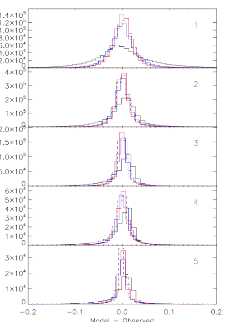
Figure 3: Residuals for all the stars in each subgrid, and all wavelengths, using the original synthetic libraries (solid black line), the corrections using $n=m=h=1$ (solid dashed line), those for $n=2$, $m=0$, $h=1$ (red), and those for $n=2$, $m=0$, $h=0$ (blue).

Table 2: Standard deviation between the original and updated par.

Grid	$T_{\rm eff}$	$\log g$	[Fe/H]	MILES stars
	(K)	(cm s2)	(dex)	surviving
1	94	0.48	0.26	166
2	98	0.31	0.19	337
3	128	0.19	0.17	118
4	616	0.30	0.51	45
5	783	0.19	0.39	19

The parameters provided with MILES (Cenarro et al. 2007) have been compiled from the literature, and subsequently homogenised by identifying and removing systematics across data sets (Cenarro et al. 2001). The metallicities in this compilation are mainly from high-resolution studies, and therefore reflect measurements from iron lines. Our model spectra have simply solar scaled metal abundances and, interestingly, if the corrections introduced are independent of [Fe/H], i.e. $h=0$, our rederived metallicities are systematically higher than those in the MILES catalogue for metal-poor stars. With $h>0$, such a trend disappears, as the corrections partially account for the relative strengthening of the features produced by $\alpha-$elements relative to iron.

The polynomial fitting using the algorithm described in Section 2 was then repeated using the original grid of synthetic spectra and the rederived atmospheric parameters. New model fluxes for the MILES stars were recalculated by quadratic Bezier interpolation, and the residuals between these and the observed fluxes are displayed in Fig. 3.

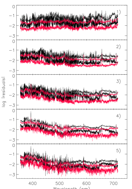
Figure 4: The lines show the 25% and 75 % percentiles of the decimal logarithm of the absolute value of the residuals between the model and the observed spectra for the original theoretical library (black) and the 2nd-order corrected (1st-order for the warmest subgrid, shown in the bottom panel) library (red).

Fig. 4 shows the 25% and the 75% percentiles of the absolute value of the residuals for each of the subgrids as a function of wavelength. The black lines are the original results for the theoretical library, and the red lines correspond to the same percentiles for the corrected library. Not only the residuals are decreased for essentially all the parameter space, but they are also smoother with wavelength for cool spectral types.

Fig. 5 illustrates the same results from a different perspective. The absolute value of the residuals are now shown for individual stars for each subgrid. Each star has two data points in the plot, at the same location, differing only on the size and type of symbol: open circles correspond to the original synthetic grid, and filled circles to the second-order corrected grid. The corrected library is in generally closer to the observations, but not in all cases, as permitted by the least-squares approach.

To ensure that we are not overfitting the data, the polynomial modelling was repeated using only 2/3 of the stars, examining the changes in the residuals between the corrected grid and the observations for the remainder of the stars. This test showed also a significant reduction in the residuals, in line with the results obtained when fitting the complete sample.

5 External check

A sanity check of the empirical spectral energy distributions can be done by using stars with reliable spectrophotometric calibrations. We have chosen three key stars: the Sun, BD $+17$ 4718, and Vega. Our choice of atmospheric parameters for these stars, compiled from the literature, are shown in Table 3. The data are from the calibration archive for HST, calspec (Bohlin 2008, 2010, and references therein); they come from HST observations for all the stars but the Sun, which are from the compilation by Colina, Bohlin, & Castelli (1996). We have dereddened the spectrum of BD $+17$ 4718 according to the prescription by Fitzpatrick & Masa (Fitzpatrick 1999), using $A_{V}/E(B-V)=3.1$, consistent with the corrections applied to MILES.

Figure 5: Absolute value of the residuals for individual stars in each of the grids. The open circles correspond to the original grid of synthetic spectra, and the filled circles to the grid corrected with first-order polynomials. The residuals are projected onto the $T_{\rm eff}$–$\log g$ plane for all five grids, and also for the $T_{\rm eff}$–[Fe/H] plane for grid #2 in the bottom-left panel.

Table 3: Testing stars.

Star	$T_{\rm eff}$	$\log g$	[Fe/H]	E(B-V)	References
	(K)	(cm s2)	(dex)	(mag)
Sun	5777	4.44	$0.0$	0.00	Stix (2004)
BD $+174708$	6141	3.87	$-1.7$	0.01	Ramírez et al. (2006)
Vega	9620	3.98	$-0.7$	0.00	García-Gil et al. (2005)

We warn the readers that parameters adopted for BD $+17$ 4708 and Vega rely on the HST spectrophotometry for these stars and model fluxes based on Kurucz atmospheres, and therefore the excellent agreement found for our purely theoretical fluxes is somewhat facilitated. The test is only completely fair for the Sun, as this is the only star in this group with parameters that are truly independent from model atmospheres (and have negligible errors), but the others are included as they may help to confirm the conclusions found from the examination of the solar case.

Fig. 6 compares the predicted spectral energy distributions, obtained by linear interpolation in a) our purely theoretical grid of model spectra (red line in left-hand panels), and b) our empirically calibrated grid (red line in right-hand panels). The interpolated spectra have also been smoothed to approximate the lower resolution of the HST spectrophotometry, with a FWHM resolving power $\lambda/\delta\lambda\sim 1000$. Overall, the calibrated grid performs slightly better than the purely theoretical grid in some regions, but the opposite is true in others.

This result suggests that there may be some systematic differences between the flux scale adopted for HST calibration and that of the MILES library, and the corrections derived from MILES may not be widely applicable. To keep a perspective, we note that systematic and random errors in the MILES fluxes were estimated to be about 2 and 3 %, respectively, from the comparison with photometry ($B-V$) from the Lausanne data base (Mermilliod et al. 1997). A reduction in effective temperature for the solar model by 150 K – which is a typical error in this quantity to be expected for most stars (not the Sun)– would be enough to bridge the 5% gap in the red between the solar fluxes and those from the empirically corrected library.

It should be emphasised that an empirical calibration, such as the procedure described in this paper, will equally erase discrepancies between models and observations due to model deficiencies and due to systematic errors in the observations, and the latter are highly dependent on the source of the data. In the upper-right panel of Fig. 6, we also show in blue the spectra of three G2V stars included in the MILES library: HD 10307, HD 84737, and HD 13043. As expected, their fluxes are consistent with the spectrum interpolated in the corrected library. An interpolated spectrum for the solar parameters from neighbouring stars using the tool available at the MILES web site leads to the same conclusion.

It is interesting to highlight the poor matching between the original library and the observed strength of the Ca II H and K lines in BD $+17$ 4708. This mismatch, which can be directly ascribed to the use of solar abundance ratios in the models, and hence the neglect of the enhancement in $\alpha$ elements typically observed in metal-poor halo stars, is reduced somewhat after the polynomial corrections have been introduced.

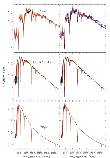
Figure 6: Observed (CALSPEC) spectrophotometry for three flux standards (Sun, BD $+174707$, and Vega; in black) compared with spectra interpolated from our grids (red lines): left-hand side graphs for the purely theoretical grid, and right-hand side for the MILES-calibrated grid. In the top right-hand panel, several spectra of solar-like stars from the MILES library are shown in blue.

6 Summary and conclusions

We present a general strategy to calibrate a set of model stellar fluxes using observations for a network a flux standards. At each frequency, the ratio of model and observed fluxes is fit by least-squares to a polynomial that depends on the atmospheric parameters. We test this scheme on the MILES stellar library, with satisfactory results: second-order corrections on effective temperature, zero-th order corrections on surface gravity, and zero-th or first-order corrections on metallicity perform well and improve significantly the agreement between the model grid and the observations, resulting in tighter and more symmetric distributions of residuals.

Seeking an external assessment of the performance of the corrections, we take a close look at the spectra of three well-known flux standards (see Bohlin 2007 and references therein). The result of this test is a much modest than expected improvement, showing that the purely theoretical fluxes perform better than those corrected for some wavelengths and stars. This suggests that the HST fluxes and those in the MILES library are not fully compatible, but further investigation is warranted.

The HST/STIS Next Generation Spectral Library (Gregg et al. 2005) has been recently released as part of the high-level products in the Multi-mission Archive at the Space Telescope (MAST). This library is based on observations made in cycles 10 through 13 and includes nearly 400 stars. This number is smaller than those in the MILES library and the resolution of the spectra is also lower, but the spectral coverage is wider. An application of the method presented here to this library, or if compatible with MILES, to the combination of the two libraries would be useful and is planned for the future.

References

- Allende Prieto et al. (2009) Allende Prieto, C., Hubeny, I., & Smith, J. A. 2009, MNRAS, 396, 759
- Allende Prieto et al. (2008) Allende Prieto, C., et al. 2008, AJ, 136, 2070
- Allende Prieto et al. (2006) Allende Prieto, C., Beers, T. C., Wilhelm, R., Newberg, H. J., Rockosi, C. M., Yanny, B., & Lee, Y. S. 2006, ApJ, 636, 804
- Allende Prieto (2004) Allende Prieto, C. 2004, Astronomische Nachrichten, 325, 604
- Asplund et al. (2005) Asplund, M., Grevesse, N., & Sauval, A. J. 2005, Cosmic Abundances as Records of Stellar Evolution and Nucleosynthesis, 336, 25
- Bautista (1997) Bautista M A 1997, A&AS, 122, 167–176.
- Bohlin (2007) Bohlin, R. C. 2007, The Future of Photometric, Spectrophotometric and Polarimetric Standardization, 364, 315
- Bohlin (2010) Bohlin, R. C. 2010, AJ, 139, 1515
- Bohlin & Cohen (2008) Bohlin, R. C., & Cohen, M. 2008, AJ, 136, 1171
- Bruzual & Charlot (2003) Bruzual, G., & Charlot, S. 2003, MNRAS, 344, 1000
- Castelli & Kurucz (2004) Castelli, F., & Kurucz, R. L. 2004, arXiv:astro-ph/0405087 bibitem[Cenarro et al.(2007)]2007MNRAS.374..664C Cenarro, A. J., et al. 2007, MNRAS, 374, 664
- Cenarro et al. (2001) Cenarro, A. J., Gorgas, J., Cardiel, N., Pedraz, S., Peletier, R. F., & Vazdekis, A. 2001, MNRAS, 326, 981 bibitem[Coelho et al.(2007)]2007MNRAS.382..498C Coelho, P., Bruzual, G., Charlot, S., Weiss, A., Barbuy, B., & Ferguson, J. W. 2007, MNRAS, 382, 498
- Cunto et al. (1993) Cunto W, Mendoza C, Ochsenbein F and Zeippen C J 1993 Bulletin d’Information du Centre de Donnees Stellaires, 42, 39–+.
- Fitzpatrick (1999) Fitzpatrick, E. L. 1999, PASP, 111, 63
- García-Gil et al. (2005) García-Gil, A., García López, R. J., Allende Prieto, C., & Hubeny, I. 2005, ApJ, 623, 460
- González Delgado et al. (2005) González Delgado, R. M., Cerviño, M., Martins, L. P., Leitherer, C., & Hauschildt, P. H. 2005, MNRAS, 357, 945
- Gregg et al. (2006) Gregg, M. D., et al. 2006, The 2005 HST Calibration Workshop: Hubble After the Transition to Two-Gyro Mode, 209
- Irwin (1981) Irwin, A. W. 1981, ApJS, 45, 621
- Koesterke (2009) Koesterke, L. 2009, American Institute of Physics Conference Series, 1171, 73
- Koesterke et al. (2008) Koesterke, L., Allende Prieto, C., & Lambert, D. L. 2008, ApJ, 680, 764
- Le Borgne et al. (2004) Le Borgne, D., Rocca-Volmerange, B., Prugniel, P., Lançon, A., Fioc, M., & Soubiran, C. 2004, A&A, 425, 881
- Mermilliod et al. (1997) Mermilliod, J.-C., Mermilliod, M., & Hauck, B. 1997, A&AS, 124, 349
- Nahar (1995) Nahar S N 1995, A&A, 293, 967–977.
- Sánchez-Blázquez et al. (2006) Sánchez-Blázquez, P., et al. 2006, MNRAS, 371, 703
- Ramírez et al. (2006) Ramírez, I., Allende Prieto, C., Redfield, S., & Lambert, D. L. 2006, A&A, 459, 613
- Schiavon et al. (2000) Schiavon, R. P., Barbuy, B., & Bruzual A., G. 2000, ApJ, 532, 453 bibitem[Stix(2004)]2004suin.book…..S Stix, M. 2004, The sun : an introduction, 2nd ed., by Michael Stix. Astronomy and astrophysics library, Berlin: Springer, 2004. ISBN: 3540207414,
- Tsuji (1964) Tsuji, T. 1964, Annals of the Tokyo Astronomical Observatory, 9,
- Tsuji (1973) Tsuji, T. 1973, A&A, 23, 411
- Vazdekis et al. (2010) Vazdekis, A., Sánchez-Blázquez, P., Falcón-Barroso, J., Cenarro, A. J., Beasley, M. A., Cardiel, N., Gorgas, J., & Peletier, R. F. 2010, MNRAS, 404, 1639