Thermal conductivity in a mixed state of a superconductor at low magnetic fields

Abstract

We evaluate accurate low-field/low-temperature asymptotics of the thermal conductivity perpendicular to magnetic field for one-band and two-band s-wave superconductors using Keldysh-Usadel formalism. We show that heat transport in this regime is limited by tunneling of quasiparticles between adjacent vortices across a number of local points and therefore widely-used approximation of averaging over the circular unit cell is not valid. In the single-band case, we obtain parameter-free analytical solution which provides theoretical lower limit for heat transport in the mixed state. In the two-band case, we show that the heat transport is controlled by the ratio of gaps and diffusion constants in different bands. Presence of a weaker second band strongly enhances the thermal conductivity at low fields.

I Introduction

The thermal conductivity of a metal in the superconducting state is markedly different from its value in the normal state. The physical reason is that the Cooper pairs give no contribution to the transport of heat. Therefore heat transport occurs solely due to the quasiparticle excitations controlled by the energy gap. Due to this reason, measurements of the thermal conductivity were extensively used during last decades as a tool to probe the energy gap symmetry in various new superconducting materials.

Application of a magnetic field $H$ provides a way to generate quasiparticles in a type-II superconductor. In a s-wave superconductor at $T\ll T_{c}$, the quasiparticles are localized near the vortex cores and thermal conduction perpendicular to the magnetic field is due to tunneling between adjacent vortices. Thermal conductivity in the mixed state of superconductors was extensively studied in the past experimentally LowellSousaJLTP70 ; VinenPhysica71 ; KesJLTP75 and theoretically PeschZPhysik74 ; ImaiWattsJLTP77 . Early theoretical work PeschZPhysik74 ; ImaiWattsJLTP77 addressed superconductors in diffusive regime (dirty limit) in the mixed state with a temperature gradient applied transverse to the magnetic flux. The electronic thermal conductivity was calculated using the quasiclassical time-dependent superconductivity theory, assuming homogeneous temperature gradient, using the circular-cell approximation, and averaging over the unit cell. This approach was later extended to study heat transport in various unconventional superconductors. Theory for d-wave superconductors was developed in Ref. GrafPRB96, for zero magnetic field and in Refs. KubertHPRL98, ; VorontsovVekhterPRB07, for the mixed state. More recently, with the discovery of magnesium diboride (MgB₂), theory was extended to the case of multiband superconductivity KusunosePRB02 . Discovery of pnictides, with possibly unconventional pairing mechanism due to spin fluctuations leading to the so-called $s_{\pm}$ pairing state, motivated extension of heat transport theory MishraPRB09 taking into account multiband superconductivity and resonant interband impurity scattering. Many recent experimental studies reconsider old superconductors, such as NbSe₂ BoakninPRL03 , and addressed novel superconductors, such as borocarbides (LuNi₂B₂C) BoakninPRL01 , Sr₂RuO₄ ShakeripourNJP09 , $C_{6}Yb$ SutherlandPRL07 , heavy-fermion compounds CeIrIn₅, CeCoIn₅ and UPt₃ ShakeripourNJP09 , MgB₂ SologubenkoPRB02 , pnictides Tanatar ; Reid and iron-silicides Machida . Being very sensitive to the gap structure, thermal transport at low magnetic fields varies considerably for different compounds.

In this paper we reconsider more accurately the problem of the thermal conductivity across the magnetic fields for s-wave superconductors. The case of s-wave superconductor is a standard reference, all other situations are compared with this case. Surprisingly, an accurate result for the low-field asymptotics of the thermal conductivity was never derived. The widely-used circular unit cell approximation does not give correct result in low magnetic fields because it misses essential physics. Namely, as the local thermal conductivity is strongly inhomogeneous, the heat transport is limited by tunneling between adjacent vortices across certain local points in the vortex lattice unit cell (bottlenecks). This leads to general low-field asymptotics of the electronic thermal conductivity, $\kappa\propto\exp(-\beta\sqrt{B_{c2}/B})$, where $B_{c2}$ is the upper critical field.VinenPhysica71 Surprisingly, the theoretical value of the numerical constant $\beta$ is not available neither for clean nor for dirty s-wave superconductors. For clean case, we provide estimate for this numerical constant using asymptotics of the Bogolyubov wave functions of the localized states at zero energy and microscopic value of the upper critical field. In the dirty case we were able to perform more quantitative analysis using the Keldysh-Usadel formalism. We calculate the thermal conductance at low temperature and low magnetic field for single- and two-band superconductors in the dirty limit. In this regime we obtain parameter-free analytical solution in a single-band case which provides theoretical lower limit for heat transport in the mixed state. We find that in dirty case the low-field thermal conductivity is drastically suppressed in comparison with clean case. Further, we generalize the developed formalism to a two-band superconductor, taking MgB₂ as an example.

II Tunneling of quasiparticles between vortex cores in clean isotropic superconductor

The electronic transverse thermal conductivity in mixed state at low temperatures and fields is determined by the probability quasiparticle tunneling between the cores of neighboring vortices. In this section we evaluate this quantity with exponential accuracy for clean isotropic superconductors. Even though this estimate is very straightforward and could be done long time ago, to our great surprise, we did not succeed to find it in the literature.

The Bogolyubov wave function of the localized state in the vortex core at $E=0$ decays as WaveFun

$$\Psi(r)\propto\exp(-r/\xi_{\Delta}),\text{ }\xi_{\Delta}=v_{F}/\Delta$$ (1)

where $\Delta$ is the superconducting gap and $v_{F}$ is the Fermi velocity. Therefore, the probability of tunneling between the vortex cores separated by distance $a=\sqrt{2\Phi_{0}/\sqrt{3}B}$ can be estimated as

$$P\!\propto\!|\Psi(a)|^{2}\!\propto\!\exp(-2a/\xi_{\Delta})\!=\!\exp\left(\!-\sqrt{\frac{8\Phi_{0}}{\sqrt{3}B\xi_{\Delta}^{2}}}\right)$$ (2)

The upper critical field $B_{c2}$ for a clean isotropic superconductor at $T=0$ is given by Hc2Clean

$$B_{c2}=\frac{e^{2}}{4\gamma}\frac{\Phi_{0}}{2\pi\xi_{0}^{2}},\ \xi_{0}=\frac{v_{F}}{2\pi T_{c}}$$ (3)

with $\gamma=\exp(0.5772)=1.781$ being the Euler constant. Using also the BCS relation $\pi T_{c}=\gamma\Delta$, we evaluate

$$2\sqrt{\frac{2\Phi_{0}}{\sqrt{3}B_{c2}\xi_{\Delta}^{2}}}=\sqrt{\frac{16\pi}{\sqrt{3}\gamma e^{2}}}\approx 1.486.$$

This allows us to represent the tunneling probability (2) as

$$P\!\propto\!\exp\left(\!-\sqrt{\frac{16\pi}{\sqrt{3}\gamma e^{2}}\frac{B_{c2}}{B}}\right)\!\approx\!\exp\left(\!-1.486\sqrt{\frac{B_{c2}}{B}}\right).$$ (4)

This result also determines the low-field asymptotics of the electronic thermal conductivity of clean isotropic superconductor. The constant in the exponent is obviously sensitive to anisotropy of Fermi surface. A more quantitative analysis which would include also evaluation of the preexponential factor requires much more complicated microscopic kinetic theory for clean limit. In the following sections we make quantitative calculations of thermal transport at low fields for dirty superconductor.

III The formalism: thermal transport in dirty superconductors within quasiclassical Keldysh-Usadel model

Our study is based on the quasiclassical Keldysh-Usadel formalism LO ; Rammer ; Belzig which was developed to describe nonequilibrium properties of dirty superconductors. Below we will reproduce the main relations of this formalism needed for our derivations. Within this formalism a superconductor is described by the Green’s function

$$G=\left(\begin{array}[]{cc}{\hat{G}}^{R}&{\hat{G}}^{K}\\ 0&{\hat{G}}^{A}\end{array}\right),$$ (5)

where in dirty limit the retarded (advanced) Green’s functions $G^{R(A)}$ satisfy the Usadel equationUsadel

$$-\hbar D\nabla({\hat{G}}^{R(A)}\nabla{\hat{G}}^{R(A)})=\left[iE\hat{\tau}_{3}+\hat{\Delta},{\hat{G}}^{R(A)}\right].$$ (6)

Here $E$ is quasiparticle energy, $D$ is the electronic diffusion coefficient, $\Delta$ is the pair potential

$$\hat{\Delta}=\left(\begin{array}[]{cc}0&\Delta\\ \Delta^{\ast}&0\end{array}\right),$$ (7)

${\hat{G}^{K}}={\hat{G}^{R}}\hat{f}-\hat{f}{\hat{G}}^{A}$, $\hat{f}$ is the distribution function, ${\hat{G}^{R}=\hat{\tau}_{3}G+\hat{\tau}_{1}F}$, ${\hat{G}^{A}=-\hat{\tau}_{3}\hat{G}^{R{\dagger}}\hat{\tau}_{3}}$, where $G$ and $F$ are the normal and anomalous Green’s functions and ${\hat{\tau}_{i}}$ are Pauli matrices.

Thermal current is given by

$$\mathbf{J}_{th}=\frac{N_{0}D}{{4}}\int{E\mathrm{Tr}}\left[{\hat{\tau}_{3}\left({\hat{G}^{R}\nabla\hat{G}^{K}+\hat{G}^{K}\nabla\hat{G}^{A}}\right)}\right]{dE},$$ (8)

where $N_{0}$ is the normal density of states the Fermi level. Writing $\hat{f}=f_{L}\hat{1}+f_{T}\hat{\tau}_{3}$ , where ${f_{L}}$ and $f_{T}$ are odd and even in energy components of the distribution function, one can rewrite the thermal current in the form Chandra

$$\mathbf{J}_{th}=N_{0}\int{E}\left[D_{L}\left(E\right)\nabla f_{L}\left(E\right)+\mathrm{Im}\mathbf{J}_{E}f_{T}\right]{dE},$$ (9)

where

$$D_{T} =D\left[\left(\mathrm{Re}G\right)^{2}+\left(\mathrm{Re}F\right)^{2}\right],$$

$$D_{L} =D\left[\left(\mathrm{Re}G\right)^{2}-\left(\mathrm{Im}F\right)^{2}\right]$$

are the energy-dependent spectral diffusion coefficients and $\mathrm{Im}\mathbf{J}_{E}$ is the spectral supercurrent given by $\mathrm{Im}\mathbf{J}_{E}=\frac{1}{4}{\mathrm{Tr}}[{\hat{\tau}_{3}({\hat{G}^{R}\mathbf{\nabla}\hat{G}^{R}-\hat{G}^{A}\mathbf{\nabla}\hat{G}^{A}})}]=\mathrm{Im}F^{R}\mathrm{Re}F^{R}{\nabla\chi}$, where ${\chi}$ is the superconducting phase. In the mixed state all quantities are spatially inhomogeneous (coordinate dependences are dropped for brevity). Functions $f_{L}$ and $f_{T}$ satisfy the following kinetic equations Rammer ; Belzig

$$\nabla\left(D_{T}\nabla f_{T}\right)+\mathrm{Im}\mathbf{J}_{E}\nabla f_{L} =2Rf_{T},$$ (10)

$$\nabla\left(D_{L}\nabla f_{L}\right)+\mathrm{Im}\mathbf{J}_{E}\nabla f_{T} =0.$$ (11)

where $R=\frac{1}{4}Tr\left[\hat{\Delta}({\hat{G}^{R}+\hat{G}^{A}})\right]$. In thermal equilibrium $f_{L}=\tanh\left(E/2k_{B}T\right)$ and $f_{T}=0$. The thermal conductivity components are defined as

$$\kappa_{\alpha}=\langle J_{th,\alpha}\rangle/\langle\nabla_{\alpha}T\rangle,$$ (12)

where $\langle{\mathbf{\nabla}}T\rangle$ is the average temperature gradient and $\alpha=(x,y,z)$.

In the following, we shall use the standard $\theta$-parametrization, ${\hat{G}^{R}}(\mathbf{r})=\hat{\tau}_{3}\cos[\theta(\mathbf{r})]+\hat{\tau}_{1}\sin[\theta(\mathbf{r})]$ in which the Usadel equation has the following form Watts ; GK

$$D\left(\mathbf{\nabla}^{2}\theta-p^{2}\cos\theta\sin\theta\right)+2\Delta\cos\theta+2iE\sin\theta=0$$ (13)

where $\mathbf{p}(\mathbf{r})=\mathbf{\nabla}\phi-(2\pi/\Phi_{0})\mathbf{A}$ is superconducting momentum (within circular cell approximation $p=1/r-r/r_{s}^{2}$, $r_{s}=\sqrt{\Phi_{0}/\pi H}$). The selfconsistency equation has the form

$$\Delta\ln\frac{T}{T_{c}}=\!\frac{T}{T_{c}}\sum_{\omega}\!\left(\sin\theta-\frac{\Delta}{\omega}\right)\!$$ (14)

The diffusion coefficients in the $\theta$-parametrization are given by the expressions $D_{T}(E,\mathbf{r})=D\cosh^{2}\left(\mathrm{Im}[\theta(E,\mathbf{r})]\right)$, $D_{L}(E,\mathbf{r})=D\cos^{2}\left(\mathrm{Re}[\theta(E,\mathbf{r})]\right)$.

IV Thermal transport in the vortex state at low fields

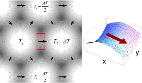
Figure 1: Left: Graylevel map of the local thermal resistance $\propto 1/D_{L}(0,\mathbf{r})$ in the vortex lattice. Light regions correspond to low thermal resistance. Arrows illustrate heat flow in the bottleneck regions. Right: Three-dimensional plot of the local thermal resistance in the bottleneck region marked by rectangle in the left picture.

We consider a superconductor in low magnetic field, $B\ll B_{c2}$. We assume an ideal triangular vortex lattice of vortex lines and study thermal transport in the direction perpendicular to the field. The local thermal conductivity is mostly determined by the diffusion constant $D_{L}(E,\mathbf{\ r})$ at low energies. This quantity is very inhomogeneous in the vortex state. It has maxima at the vortex cores and rapidly drops away from the cores reflecting localization of quasiparticles in the core regions. This means that the local thermal resistance $\propto 1/D_{L}(0,\mathbf{r})$ is maximal at the boundaries of the lattice unit cell. In such situation the temperature is mostly homogeneous within the unit cells and only changes in the boundary regions between the cells, see Fig. 1. This means that thermal transport occurs via “bottlenecks“, saddle points of $D_{L}(E,\mathbf{r})$. Our purpose is to evaluate average thermal conductivity limited by these bottlenecks. Since in the vicinity of bottlenecks, the spectral supercurrent $\mathrm{Im}\mathbf{J}_{E}$ vanishes by symmetry, the expression for local energy current simplifies and has the form: $\mathbf{J}_{th}(\mathbf{r})\approx N_{0}\int dEED_{L}\mathbf{\nabla}f_{L}$.

We start with evaluation of the diffusion constant $D_{L}(E,\mathbf{r})$ which is determined by the real part of the Green’s function $\theta(E,\mathbf{r})$. For an isolated vortex, at distances $r\!\gg\!\xi$ from its core we can present $\Delta$ and $\theta$ as $\theta(\mathbf{r})=\theta_{0}+\tilde{\theta}(\mathbf{r})$, $\Delta(\mathbf{r})=\Delta_{0}+\tilde{\Delta}(\mathbf{r})$ where $\Delta_{0}$ and $\theta_{0}$ are the equilibrium values at zero magnetic field, $\tan\theta_{0}\!=\!i\Delta_{0}/E$ and $\tilde{\theta}(\mathbf{r})\!=\!\tilde{\theta}_{r}(\mathbf{r})\!+\!i\tilde{\theta}_{i}(\mathbf{r})$ is small correction. For $E\ll\Delta_{0}$ , $\theta_{0}\approx\pi/2\!+\!iE/\Delta_{0}$, therefore the energy-diffusion constant in this region $D_{L}(E,\mathbf{r})\!\approx\!D\tilde{\theta}_{r}^{2}$. The real and imaginary parts of $\tilde{\theta}$ obey the following equations

$$D\mathbf{\nabla}^{2}\tilde{\theta}_{r}-D\frac{E^{2}+\Delta_{0}^{2}}{E^{2}-\Delta_{0}^{2}}p^{2}\tilde{\theta}_{r}-2\sqrt{\Delta_{0}^{2}-E^{2}}\tilde{\theta}_{r}=0,$$ (15)

$$D\mathbf{\nabla}^{2}\tilde{\theta}_{i}-D\frac{E^{2}+\Delta_{0}^{2}}{E^{2}-\Delta_{0}^{2}}p^{2}\tilde{\theta}_{i}-2\sqrt{\Delta_{0}^{2}-E^{2}}\tilde{\theta}_{i}$$

$$=\frac{2E\tilde{\Delta}}{\sqrt{\Delta_{0}^{2}-E^{2}}}-D\frac{E\Delta_{0}}{\Delta_{0}^{2}-E^{2}}p^{2},$$ (16)

where $p=1/r$ is the gauge-invariant phase gradient. For an isolated vortex $\tilde{\theta}_{r}$ and $\tilde{\theta}_{i}$ have qualitatively different behavior at large distances for $E<\Delta_{0}$: $\tilde{\theta}_{i}$ decays as $p^{2}\propto 1/r^{2}$ and $\tilde{\theta}_{r}$ decays exponentially

$$\tilde{\theta}_{v,r}(r) =C_{v}\frac{\exp(-k_{\xi}r)}{\sqrt{k_{\xi}r}},$$ (17)

$$k_{\xi}(E) =\sqrt{2}\left(\Delta_{0}^{2}-E^{2}\right)^{1/4}/\sqrt{D}.$$

Evaluation of numerical constant requires solution of full nonlinear problem. Numerical solution by the method described GK provides $C_{v}\approx 4.2$. In the vortex lattice away from the core regions $\tilde{\theta}_{r}$ can be represented as a sum of contributions from individual vortices

$$\tilde{\theta}_{\mathrm{lat},r}(\mathbf{r})\!\approx\!\sum_{\mathbf{R}}\tilde{\theta}_{v,r}\left(\mathbf{r}\!-\!\mathbf{R}\right)\!=\!\sum_{\mathbf{R}}C_{v}\frac{\exp(-k_{\xi}|\mathbf{r}\!-\!\mathbf{R}|)}{\sqrt{k_{\xi}|\mathbf{r}-\mathbf{R}|}},$$ (18)

where $\mathbf{R}$ are the vortex coordinates. In particular, for triangular lattice $\mathbf{R}=(a/2+ma+na/2,n\sqrt{3}/2)$ where $a=\sqrt{2\Phi_{0}/\sqrt{3}B}$ is the lattice constant and $m$ and $n$ are integers.

At small field thermal transport is determined by energy flow via bottlenecks, saddlepoints of $D_{L}(E,\mathbf{r})$ at boundaries of the lattice unit cell. Near the bottleneck point, $(x,y)=(0,0)$, we can keep only contribution from two neighboring vortices located at $(\pm a/2,0)$ which gives

$$\tilde{\theta}_{\mathrm{lat},r}(\mathbf{r})\approx\frac{2C_{v}}{\sqrt{k_{\xi}a/2}}\exp\left(-k_{\xi}a/2\right)\cosh\left(k_{\xi}x\right)\exp(-k_{\xi}y^{2}/a)$$ (19)

and

$$D_{L}(E,\mathbf{r})\approx D\frac{8C_{v}^{2}}{k_{\xi}a}\exp\left(-k_{\xi}a\right)\cosh^{2}\left(k_{\xi}x\right)\exp(-2k_{\xi}y^{2}/a).$$ (20)

Using also quasiequilibrium approximation for the gradient of $f_{L}(E,\mathbf{r})$, $\nabla_{x}f_{L}(E,\mathbf{r})\approx-\cosh^{-2}(E/2k_{B}T)(E/2k_{B}T^{2})\nabla_{x}T(\mathbf{r})$, we obtain the heat flow near the bottleneck $J_{\mathrm{th},x}(\mathbf{r})\approx-\kappa_{x}(\mathbf{r})\nabla_{x}T(\mathbf{r})$, where the local thermal conductivity $\kappa_{x}(\mathbf{r})$ is given by

$$\kappa_{x}(\mathbf{r})\approx 8C_{v}^{2}DN_{0}\int_{-\infty}^{\infty}dEE\frac{\exp\left(-k_{\xi}a\right)}{k_{\xi}a}\cosh^{2}\left(k_{\xi}x\right)\exp\left(-\frac{2k_{\xi}y^{2}}{a}\right)\frac{E/2k_{B}T^{2}}{\cosh^{2}\left(E/2k_{B}T\right)}.$$

At low temperatures $T<\Delta_{0}\xi/a$ the main contribution to the energy integral comes from the region $E\lesssim T$. This allows us to neglect the energy dependence of $k_{\xi}(E)$ and replace $k_{\xi}(E)\rightarrow k_{\xi 0}=\sqrt{2\Delta_{0}/D}=1/\xi_{\Delta}$. In this case, using $\int_{-\infty}^{\infty}x^{2}\cosh^{-2}\!x\ dx=\pi^{2}/6$, we obtain

$$\kappa_{x}(\mathbf{r})=\frac{16\pi^{2}}{3}C_{v}^{2}k_{B}^{2}TN_{0}D\frac{\exp\left(-k_{\xi 0}a\right)}{k_{\xi 0}a}$$

$$\ \times\cosh^{2}\left(k_{\xi 0}x\right)\exp\left(-\frac{2k_{\xi 0}y^{2}}{a}\right).$$ (21)

Near the bottleneck region the local thermal conductivity has a form $\kappa(x,y)=\kappa_{0}F_{x}(x)F_{y}(y)$, where the function $F_{x}(x)=\cosh^{2}\left(k_{\xi 0}x\right)$ has minimum at $x=0$ and $F_{y}(y)=\exp\left(-2k_{\xi 0}y^{2}/a\right)$ has maximum at $y=0$. The total flow per unit length along the field through the bottleneck is given by

$$I_{th}\approx\kappa_{0}F_{x}(x)\left[\int_{-\infty}^{\infty}F_{y}(y)dy\right]\nabla_{x}T.$$ (22)

Energy conservation requires that $I_{th}$ has to be $x$-independent. Therefore, the temperature drop $\Delta T$ across the bottleneck can be evaluated as

$$\Delta T\approx\frac{\int_{-\infty}^{\infty}F_{x}^{-1}(x)dx}{\kappa_{0}\int_{-\infty}^{\infty}F_{y}(y)dy}I_{th}$$ (23)

meaning that the total thermal conductance through this region $K=I_{th}/\Delta T$ can be evaluated as

$$K=\kappa_{0}\frac{\int_{-\infty}^{\infty}F_{y}(y)dy}{\int_{-\infty}^{\infty}F_{x}^{-1}(x)dx}=\frac{8\pi^{5/2}C_{v}^{2}}{3\sqrt{2}}k_{B}^{2}TN_{0}D\frac{\exp\left(-k_{\xi 0}a\right)}{\sqrt{ak_{\xi 0}}}.$$ (24)

Evaluating the total average energy flow density

$$J_{th}=\frac{I_{th}+I_{th}/4}{a\sqrt{3}/2}=\frac{5}{2\sqrt{3}}K\frac{\Delta T}{a},$$ (25)

we obtain the final result for the low-field/low-temperature limit for the thermal conductivity in the vortex-lattice state

$$\kappa/T \approx\frac{10\sqrt{2}\pi^{5/2}C_{v}^{2}}{3\sqrt{3}}k_{B}^{2}N_{0}D\frac{\exp\left(-k_{\xi 0}a\right)}{\sqrt{k_{\xi 0}a}}$$

$$=\frac{10\sqrt{2}\pi^{5/2}C_{v}^{2}}{3\sqrt{3}}k_{B}^{2}N_{0}D\frac{\exp\left(-\sqrt{(8\pi/\sqrt{3})B_{c2}/B}\right)}{\left((8\pi/\sqrt{3})B_{c2}/B\right)^{1/4}}$$ (26)

where we used relations $B_{c2}=\Phi_{0}k_{\xi 0}^{2}/4\pi$ and $k_{\xi 0}a=\sqrt{(8\pi/\sqrt{3})B_{c2}/B}$.

Introducing the thermal conductivity in the normal state $\kappa_{N}=\frac{\pi^{2}}{3}k_{B}^{2}N_{0}DT,$ we rewrite the final result in the form

$$\frac{\kappa}{\kappa_{N}} \approx 10\sqrt{\frac{2\pi}{3}}C_{v}^{2}\frac{\exp\left(-\sqrt{(8\pi/\sqrt{3})B_{c2}/B}\right)}{\left((8\pi/\sqrt{3})B_{c2}/B\right)^{1/4}}$$

$$\approx 130\left(\frac{B}{B_{c2}}\right)^{1/4}\exp\left(-3.81\sqrt{\frac{B_{c2}}{B}}\right).$$ (27)

This parameter-free analytical result provides theoretical lower limit for the heat transport in the mixed state in an isotropic dirty s-wave superconductor at low field. The constant $3.81$ in the exponent is significantly higher than the constant $1.486$ which we evaluated for the clean case (4) meaning that the scattering drastically suppresses the quasiparticle thermal conductivity at low fields.

V Discussion of experiment

Rather limited set of experimental data is available on electronic contribution to the thermal conductivity at low temperatures and low magnetic fields, since phonon contribution should be accurately subtracted in this regime. To our knowledge, the only experimental data on electronic thermal conductivity which clearly demonstrate low-field/low-temperature behavior expected for an s-wave superconductor are reported for Nb in Refs. LowellSousaJLTP70, ; VinenPhysica71, and for V₃Si in Ref. BoakninPRL03, . In these experiments the samples were in the clean limit. In Ref. VinenPhysica71, the electronic thermal conductivity was fitted by the expression $\kappa\propto\exp(-\beta\sqrt{B_{c2}/B})$ for values of $B$ up to about $B_{c2}/3$, with $\beta=1.66$. This number is slightly higher than our estimate of $\beta=1.486$ in Eq. (4). This difference can be explained by the influence of impurity scattering. The shape of field dependence of thermal conductivity for V₃Si reported in Ref. BoakninPRL03, is in qualitative agreement with the predicted exponential dependence, however the quantitative analysis was not made and the value of $\beta$ was not explicitly extracted. In a field $B=B_{c2}/20$ the value of $\kappa\approx 2.5\cdot 10^{-3}\kappa_{N}$ provided in Ref. BoakninPRL03, exceeds our dirty-limit estimate, Eq. (27), by about two orders of magnitude. This discrepancy can be naturally attributed to the fact that measured V₃Si samples were in the clean limit. The magnitude of thermal conductivity at not very small magnetic fields is in good qualitative agreement with calculations made for the clean limit using the Landau-level expansion and assuming homogeneous temperature gradient Dukan . To our knowledge, there are no data available on electronic thermal conductivity of dirty s-wave superconductors in the low-field/low-temperature limit. In available measurements of alloys LowellSousaJLTP70 and dirty Nb samples KesJLTP75 the thermal conductivity at low fields and temperatures is dominated by phonons and separating electronic contribution is a challenging task.

VI Extension to a two-band superconductor

Here we extend the above formalism to a two-band superconductor. At present, the most established example of such system is MgB₂, which is characterized by two electronic bands: $\pi$-band and $\sigma$-band, see, e. g.  recent review Ref. XiReview08, . The quasi-two-dimensional $\sigma$-band is characterized by stronger superconductivity than the three-dimensional $\pi$ -band. Heat transport in a two-band superconductor was studied theoretically in Ref. KusunosePRB02, assuming clean limit conditions and using the averaging over unit cell method PeschZPhysik74 ; ImaiWattsJLTP77 . In the dirty limit, theory of density of states in the mixed state and the upper critical field for MgB₂ was developed in Refs. MgB2-DoS, ; MgB2-Hc2, . Below we extend the calculations of the heat transport presented above, to the case of a diffusive two-band superconductor, taking MgB₂ as an example.

In the presence of two electronic bands with different energy gaps, low-temperature behavior of thermal transport is determined by the band with lower gap ($\pi$-band). Still, the generalization from single-band to two-band case involves not simply renormalization of the energy gap, but also correction to the asymptotic behavior of Green’s function in the $\pi$ -band and to the upper critical field.

The Usadel equation for the $\pi$-band reads

$$D_{\pi}\left(\mathbf{\nabla}^{2}\theta_{\pi}\!-\!p^{2}\cos\theta_{\pi}\sin\theta_{\pi}\right)\!+\!2\Delta_{\pi}\cos\theta_{\pi}\!+\!2iE\sin\theta_{\pi}\!=\!0,$$ (28)

where $D_{\pi}$ and $\Delta_{\pi}(\mathbf{r})$ are the diffusion constant and gap for the $\pi$-band. Similar to a single-band case, asymptotics of the Green’s function in the $\pi$-band at large distance from the vortex core is given by

$$\tilde{\theta}_{\pi,r}(r)=C_{\pi}\frac{\exp(-k_{\pi}r)}{\sqrt{k_{\pi}r}}.$$ (29)

with

$$k_{\pi}(E)=\sqrt{2}\left(\Delta_{\pi 0}^{2}-E^{2}\right)^{1/4}/\sqrt{D_{\pi}}.$$

The main exponential dependence of the zero-energy Green’s function at the bottleneck point is $\propto\exp(-k_{\pi 0}a)$, where $k_{\pi 0}=k_{\pi}(0)=\sqrt{2\Delta_{\pi 0}/D_{\pi}}$, which gives

$$k_{\pi 0}a =\sqrt{B_{\pi}/B},$$ (30)

$$B_{\pi} =\frac{2\Delta_{\pi 0}}{D_{\pi}}\frac{2\Phi_{0}}{\sqrt{3}}.$$ (31)

Therefore, the magnetic field dependence of thermal conductivity is determined by the field scale $B_{\pi}$ and can be presented in the form similar to Eq. (27),

$$\frac{\kappa}{\kappa_{\pi N}}\approx 10\sqrt{\frac{2\pi}{3}}C_{\pi}^{2}\frac{\exp\left(-\sqrt{B_{\pi}/B}\right)}{\left(B_{\pi}/B\right)^{1/4}},$$ (32)

where $\kappa_{\pi N}=\frac{\pi^{2}}{3}k_{B}^{2}N_{\pi}D_{\pi}T$ is the partial $\pi$-band contribution to the normal-state thermal conductivity.

To proceed further, we have to find relation between the $\pi$-band field scale $B_{\pi}$ and the upper critical field $B_{c2}$ for a two-band superconductor. The upper critical field at low temperatures, $T\ll T_{c}$, is given by MgB2-Hc2

$$B_{c2}(0)=a_{c2}B_{c2}^{s}(0),\ \ a_{c2}=\exp\left(-\frac{W_{1}\!+\!W_{2}\!-\!\ln r_{x}}{2}+\sqrt{\frac{\left(W_{1}\!+\!W_{2}\!-\!\ln r_{x}\right)^{2}}{4}\!+W_{1}\ln r_{x}}\right),$$ (33)

where indices 1 and 2 correspond to the $\sigma$ and $\pi$ bands,

$$W_{1,2}=\frac{\mp(\Lambda_{11}-\Lambda_{22})/2+\sqrt{(\Lambda_{11}-\Lambda_{22})^{2}/4+\Lambda_{12}\Lambda_{21}}}{\Lambda_{11}\Lambda_{22}-\Lambda_{12}\Lambda_{21}},$$

$\Lambda_{\alpha\beta}$ is the coupling-constant matrix, $r_{x}=\mathcal{D}_{\sigma}/\mathcal{D}_{\pi}$, $\mathcal{D}_{\sigma,\pi}$ are the diffusion constants in $\sigma$ and $\pi$ bands,

$$B_{c2}^{s}(0)=\frac{\Delta_{BCS}\Phi_{0}}{2\pi\mathcal{D}_{\sigma}}$$ (34)

is the single-band upper critical field for the $\sigma$-band, and $\Delta_{BCS}=\pi e^{-\gamma_{E}}T_{c}\approx 1.764T_{c}$ ($\gamma_{E}\approx 0.5772$ is the Euler constant).

To make estimates for MgB₂, we use the following coupling matrix elements MgB2-DoS ; MgB2-Hc2 : $\Lambda_{11}\!\approx 0.81,\ \Lambda_{22}\!\approx 0.278,\ \Lambda_{12}\!\approx 0.115,\ \Lambda_{21}\!\approx 0.091$, which gives $\!W_{1}\!\approx 0.088$ and $W_{2}\!\approx 2.56$. With such coupling matrix the two-band BCS model gives MgB2-DoS $\Delta_{\pi 0}\simeq 0.3\Delta_{\sigma 0}\simeq$ $0.177\pi T_{c}$. Since the parameter $W_{1}$ is small, typically the inequality $W_{1}|\ln r_{x}|\ll\left(W_{2}-\ln r_{x}\right)^{2}/4$ is valid. In this case one can expand Eq. (33) with respect to $W_{1}$ and obtain simple result

$$a_{c2}\approx 1+\frac{W_{1}\ln r_{x}}{W_{2}-\ln r_{x}},$$ (35)

meaning that the upper critical field is close to $B_{c2}^{s}(0)$ and is mostly determined by the coherence length of the $\sigma$-band. Using Eqs. (31), (33), and (34), we obtain the relation between $B_{\pi}$ and $B_{c2}(0)$

$$B_{\pi}=\frac{8\pi}{\sqrt{3}a_{c2}}\frac{\Delta_{\pi 0}}{\Delta_{BCS}}\frac{\mathcal{D}_{\sigma}}{\mathcal{D}_{\pi}}B_{c2}(0),$$ (36)

which presents the main result of this section. This scale has to be compared with the scale $(8\pi/\sqrt{3})B_{c2}(0)$ for the single-band case.

In order to determine the pre-exponential factor $C_{\pi}$ in Eqs. (29) and (32), we have to calculate the Green’s function $\tilde{\theta}_{\pi,r}(r)$, which requires solution of the full two-band Usadel problem, as described in Ref. MgB2-DoS, . An important parameter is the ratio of diffusion coefficients in two bands $r_{x}$ . For illustration, we consider two cases here: $r_{x}=1$ and $0.2$, for which the ratios of the coherence lengths in the two bands are $\xi_{\pi}/\xi_{\sigma}=\sqrt{(D_{\pi}/D_{\sigma})(\Delta_{\sigma 0}/\Delta_{\pi 0})}=1.83$ and 4.1. For these two cases we compute $B_{\pi}\approx 0.32(8\pi/\sqrt{3})B_{c2}(0)$, $C_{\pi}\approx 3.6$ for $r_{x}=1$ and $B_{\pi}\approx 0.065(8\pi/\sqrt{3})B_{c2}(0)$, $C_{\pi}\approx 2.9$ for $r_{x}=0.2$. This gives

$$\ \frac{\kappa}{\kappa_{\pi N}} \!\approx\!130\left(\frac{B}{B_{c2}(0)}\right)^{1/4}\exp\left(-2.15\sqrt{\frac{B_{c2}(0)}{B}}\right)\ \text{,\ }r_{x}=1$$

$$\!\approx\!130\left(\frac{B}{B_{c2}(0)}\right)^{1/4}\!\exp\left(\!-0.98\sqrt{\frac{B_{c2}(0)}{B}}\right)\text{,\ }r_{x}\!=\!0.2$$

We can see that the field scale in the two-band case is strongly reduced in comparison with the single-band case leading to large enhancement of the thermal conductivity at low fields. This reduction is mostly caused by the smaller energy gap in the $\pi$ band. Another factor which may contribute is possible large value of the diffusion constant $D_{\pi}$. The smaller field scale caused by the larger coherence length in the $\pi$-band is an established feature and important fingerprint of the two-band superconductivity in MgB₂. This small scale was experimentally observed not only in the thermal conductivity SologubenkoPRB02 , but also in the specific heat SpecHeatMgB2 and flux-flow resistivity ShibataPRB03 . For the magnetic field applied along c-axis it is 3-5 times smaller than $B_{c2}$. In this case, the low-field regime described by Eq. (32) is expected at fields $<B_{c2}/30\approx 100$G. Unfortunately, most experimental data of Ref. SologubenkoPRB02, are presented for higher magnetic fields.

We shall note that in available MgB₂ single crystals estimates suggest that the $\sigma$ band is in the clean limit. However, our results should be qualitatively applicable even in this case. The reason is that dominant contribution comes from the $\pi$-band which is in the dirty limit, as argued in Ref. MgB2-DoS, where the low-energy DoS in the vortex state of MgB₂ was calculated.

In summary, we have readdressed the problem of the heat transport of a superconductor in the mixed state at low temperatures and low magnetic fields, going beyond the circular unit cell approximation. In the clean limit we estimated the numerical constant $\beta$ in the low-field asymptotics of the electronic thermal conductivity, $\kappa\propto\exp(-\beta\sqrt{B_{c2}/B})$, using the Bogolyubov wave functions of the localized states at zero energy. In the dirty limit we have performed quantitative analysis of heat transport using Keldysh-Usadel formalism and have shown that heat transport is limited by tunneling between adjacent vortices across certain local points (bottlenecks). In the isotropic s-wave superconductor we have obtained parameter-free analytical solution which provides theoretical lower limit for heat transport in the mixed state. Based on this solution, one can conclude that low-field/low-temperature thermal conductivity in the mixed state is drastically suppressed by impurity scattering. We have extended our results to the case of a two-band superconductor, taking MgB₂ as an example. In this case, we predict an enhancement of heat transport with strong dependence on the ratio of gaps and diffusion constants in different bands.

- (1) J. Lowell, J. B. Sousa, J. Low Temp. Phys., 3, 65 (1970).
- (2) W. F. Vinen, E. M. Forgan, C. E. Gough, and M. J. Hood, Physica 55, 94 (1971).
- (3) P. H. Kes, J. P. M. van der Veeken, and D. de Kierk, Journ. of Low Temp. Phys., 18, (1975).
- (4) W. Pesch, R. Watts-Tobin, and L. Kramer Z. Physik 269, 253 (1974).
- (5) S. Imai and R.J. Watts-Tobin, Journ. of Low Temp. Phys., 26 967 (1977).
- (6) M. J. Graf, S-K. Yip, J. A. Sauls, and D. Rainer, Phys. Rev. B 53, 15147 (1996).
- (7) A. B. Vorontsov and I. Vekhter, Phys. Rev. B 75, 224502 (2007).
- (8) C. Kübert and P. J. Hirschfeld, Phys. Rev. Lett. 80, 4963(1998).
- (9) H. Kusunose, T. M. Rice, and M. Sigrist, Phys. Rev. B, 66, 214503 (2002).
- (10) V. Mishra, A. Vorontsov, P. J. Hirschfeld, and I. Vekhter, Phys. Rev. B 80, 224525 (2009)
- (11) E. Boaknin, R. W. Hill, Cyril Proust, C. Lupien, and L. Taillefer, and P. C. Canfield, Phys. Rev. Lett. 87, 237001 (2001).
- (12) E. Boaknin, M. A. Tanatar, J. Paglione, D. Hawthorn, F. Ronning, R. W. Hill, M. Sutherland, L. Taillefer, J. Sonier, S. M. Hayden, and J. W. Brill, Phys. Rev. Lett. 90, 117003 (2003).
- (13) H. Shakeripour, C. Petrovic, and Louis Taillefer, New Journal of Physics, 11, 055065 (2009).
- (14) M. Sutherland, N. Doiron-Leyraud, L.Taillefer, T. Weller, M. Ellerby, and S. S. Saxena, Phys. Rev. Lett. 98, 067003 (2007)
- (15) A. V. Sologubenko, J. Jun, S. M. Kazakov, J. Karpinski, and H. R. Ott, Phys. Rev. B, 66, 014504 (2002).
- (16) M. A. Tanatar, J.-Ph. Reid, H. Shakeripour, X. G. Luo, N. Doiron-Leyraud, N. Ni, S. L. Bud’ko, P. C. Canfield, R. Prozorov, and L. Taillefer, Phys. Rev. Lett. 104, 067002 (2010).
- (17) J.-Ph. Reid, M. A. Tanatar, X. G. Luo, H. Shakeripour, N. Doiron-Leyraud, N. Ni, S. L. Bud’ko, P. C. Canfield, R. Prozorov, and L. Taillefer, Phys. Rev. B 82, 064501 (2010).
- (18) Y. Machida, S. Sakai, K. Izawa, H. Okuyama, and T. Watanabe, arXiv:1009.2432.
- (19) C. Caroli, P. -G. de Gennes, and J. Matricon, Phys. Letters 9, 307 (1964); C. Caroli and J. Matricon, Physik Kondensienten Materie 3, 380 (1965); J. Bardeen, R. Kümmel, A. E. Jacobs, and L. Tewordt, Phys. Rev. 187, 556 (1969).
- (20) L. P. Gor’kov, Zh. Eksperim. i Teor. Fiz. 37, 833 (1959) [English transl.: Soviet Phys.—JETP 10, 593 (1960)]; E. Helfand and N. R. Werthamer, Phys. Rev. 147, 288 (1966).
- (21) A.I. Larkin and Yu. N. Ovchinnikov, Zh. Exp. Teor. Fiz. 68, 1915, (1975) [Sov. Phys. JETP 41, 960 (1976)].
- (22) J. Rammer and H. Smith, Rev. Mod. Phys. 58, 323 (1986).
- (23) W. Belzig, F. K. Wilhelm, C. Bruder, G. Schön, and A. D. Zaikin, Superlattices and Microstructures, 25, 1251 (1999).
- (24) K.D. Usadel, Phys. Rev. Lett. 25, 507 (1970).
- (25) V. Chandrasekhar, In: The Physics of Superconductors, ed. by K.H.Bennemann and J.B.Ketterson, pp.55-110, Springer (2004).
- (26) R. Watts-Tobin, L. Kramer, and W. Pesch, J. Low Temp. Phys. 17, 71 (1974).
- (27) A.A. Golubov and M. Yu. Kupriyanov, J. Low Temp. Phys. 70, 83 (1988).
- (28) S. Dukan, T.P. Powell, and Z. Tesanović, Phys. Rev. B 66, 014517, (2002).
- (29) X. X. Xi, Rep. Prog. Phys. 71, 116501, (2008).
- (30) A.E.Koshelev and A.A. Golubov, Phys. Rev. Lett. 90, 177002 (2003).
- (31) A. Gurevich, Phys. Rev. B 67, 184515 (2003); A.A. Golubov and A.E.Koshelev, Phys. Rev. B 68, 104503 (2003)
- (32) Y. X. Wang, T. Plackowski and A. Junod, Physica C 355 179, (2001); F. Bouquet, R. A. Fisher, N. E. Phillips , D. G. Hinks and J. D. Jorgensen, Phys. Rev. Lett. 87 047001 (2001).
- (33) A. Shibata, M. Matsumoto, K. Izawa, Y. Matsuda, S. Lee and S. Tajima, Phys. Rev. B 68, 060501(R) (2003)