Quantum computational capability of
a 2D valence bond solid phase

Abstract

Quantum phases of naturally-occurring systems exhibit distinctive collective phenomena as manifestation of their many-body correlations, in contrast to our persistent technological challenge to engineer at will such strong correlations artificially. Here we show theoretically that quantum correlations exhibited in the two-dimensional (2D) valence bond solid phase of a quantum antiferromagnet, modeled by Affleck, Kennedy, Lieb, and Tasaki (AKLT) as a precursor of spin liquids and topological orders, are sufficiently complex yet structured enough to simulate universal quantum computation when every single spin can be measured individually. This unveils that an intrinsic complexity of naturally-occurring 2D quantum systems — which has been a long-standing challenge for traditional computers — could be tamed as a computationally valuable resource, even if we are limited not to create newly entanglement during computation. Our constructive protocol leverages a novel way to herald the correlations suitable for deterministic quantum computation through a random sampling, and may be extensible to other ground states of various 2D valence bond phases beyond the AKLT state.

1 Introduction

Daily stories about a quantum computer have earned in our mind its image as super postmodern technology based on an artificial full control of quantum systems in the highest possible precision. Most current approaches to implement a quantum computer are based on a bottom-up idea in that we intend to build it by combining key elementary objects, as well summarized by the celebrated DiVincenzo criteria [1]. The idea implies that it should be equally, i.e., reversibly, doable to both create and annihilate at will many-body correlations (or entanglement if its nonlocal character has to be emphasized) among many qubits artificially. However, despite various promising candidates for a qubit and remarkable experimental progresses in their physical implementation, this unitary control of many-body entanglement in a scalable fashion is believed to remain the hardest challenge.

On the other hand, in a historical perspective, humanity has strived to find and tame resources present naturally on the earth, rather than achieving our goal from scratch by our immediate ability. Speaking of energy resources for instance, instead of establishing self-contained energy cycle in the first place, we have learned to take advantage of more and more elaborated natural resources, e.g., from wood and water to oil and nuclear (although their sustainable use is still our long-term project). Here, based on the fact that nature realizes various quantum phases as manifestation of underlying many-body entanglement, we suggest taking a complementary, top-down vision in that we attempt to tame a resource of suitably structured entanglement, which could either exist in nature or be simulated relatively naturally within our technology.

A key point is how to live with our limited ability. Once a specific natural resource of structured many-body entanglement is provided, we are supposed to utilize only operations which just consume entanglement without its new creation, such as local measurements and local turning off of an interaction. In this regard, our approach can be best compared to hewing out an arbitrary quantum evolving system from the “carving” resource, in enhancing Feynman’s original intuition [2] about quantum simulation in a computationally universal manner. A perquisite is that we could be content with limited technology to prepare only one specific resource of structured many-body correlation, that is less demanding than the full unitary control over arbitrary correlation. Moreover, if such a resource is available as a stable ground state of a naturally-occurring system, that gives us several possibilities to prepare, such as dissipative coolings or adiabatic evolutions, in a similar way that nature presumably does. Our target of the naturally-occurring two-dimensional (2D) system is the valence bond solid (VBS) phase of spin $\tfrac{3}{2}$’s on the 2D hexagonal lattice, modeled by Affleck, Kennedy, Lieb, and Tasaki (AKLT) [3, 4], which is widely recognized as a cornerstone in condensed matter physics. Their VBS construction of the ground state in terms of the distributed spin singlets (or the valence bonds) has become one of most ubiquitous insights in quantum magnetism as well as in high-$T_{c}$ superconductivity, and leads to modern trends of spin liquids and topological orders.

It turns out here that the 2D VBS phase, represented by the AKLT ground state, provides an ideal entanglement structure of quantum many-body systems that can be suitably tamed through our limited capability to the goal of universal quantum computation. Our top-down vision is materialized conveniently in taking advantage of a conventional framework of measurement-based quantum computation (MQC). Its methods have been developed to “steer” quantum information through given many-body correlations using only a set of local measurements and classical communication, under which entanglement is just consumed without new creation. Later we extend that in a wider program to tame naturally-occurring many-body correlations.

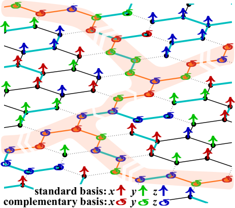
Figure 1: A scheme of quantum computation through measuring the correlations of the 2D AKLT state, a representative state of the 2D VBS phase of spin $\tfrac{3}{2}$’s on the 2D hexagonal lattice. After a random sampling which assigns every spin per site to one of three axes $x$, $y$, and $z$, the typical configuration of the outcomes enables us to choose the backbone structure (described by a shaded pinkish-orange region) along which quantum computation is deterministically simulated in terms of a quantum circuit. Our protocol harnesses a pair (depicted as a dotted bond of the hexagonal lattice) of neighboring sites where one is measured in a standard basis and the other is done in a complementary basis, to accommodate the desired structure of space-time along the region of the backbone. An emergence of the time is simulated if both two bits of information out of measurements per site are communicated to the same direction (as depicted as the double arrows), on the other hand, an emergence of the space is simulated if two bits of information are communicated to the opposite directions (as depicted as a pair of the single arrows pointing apart). The figure, reminiscent of the Feynman diagram for scattering of two elementary particles, illustrates a microscopic view of the Figure 2. The two-qubit CNOT gate is implemented in the middle region between two quantum logical wires running from the right to the left.

In the context of MQC, the so-called 2D cluster state [5] is the first and canonical instance of such an entangled state that pertains to a universal quantum computational capability when every single qubit (spin $\tfrac{1}{2}$) is measured individually and the outcomes of the measurements are communicated classically [6, 7]. Remarkably, it was already noticed in Ref. [8] that MQC on the 2D cluster state utilizes a structure of entanglement which is analogous to that of the aforementioned VBS state. Following such an observation, the tensor network states, as a class of efficiently classically parameterizable states in extending the VBS construction, has been used in Refs. [9, 10] to construct resource states of MQC, where it was indicated that a certain set of the local matrices or tensors which describe the correlations (cf. Eq. (2) in our case) can result in a quantum unital map through the single-site measurement. Notably, however, most known examples considered so far, including additionally those e.g., in Refs. [13, 11, 12, 14, 15, 16], are constructed to have such a convenient yet artificial property — as often referred as one of peculiar properties of the correlations of the 2D cluster state — that it is possible to decouple deterministically (by measurements of only neighboring sites) a 1D-chain structure that encodes the direction of a simulated time as a quantum logical wire of the quantum circuit model. This peculiarity is said to be artifact of another less realistic feature of the 2D cluster state in that it cannot be the exact ground state of any two-body Hamiltonian of spin $\tfrac{1}{2}$’s [17, 18]. Thus one cannot expect such convenience for the correlations of a genuine 2D ground state of a naturally-occurring spin system.

The main result of our paper is summarized in the following (informal) theorem and illustrated in the Figure 1. As elaborated in the text, we introduce a novel way to herald the correlations suitable for deterministic quantum computation through a random sampling, to tame for the first time the genuine 2D naturally-occurring correlation. Otherwise it has natural tendency to split an incoming information into two outgoing information because of certain symmetric nature of the three directions at every site of the 2D hexagonal lattice. This seems to be the reason why MQC on the 2D AKLT state has been an open question in a long time, although the AKLT state by the 1D spin-1 chain was shown in Ref. [11] to be capable of simulating a single quantum wire of MQC.

Theorem.

Universal quantum computation can be simulated through consuming monotonically entanglement provided as the 2D AKLT state $\left|\mathcal{G}\right\rangle$ (defined as the VBS state by a spin $\tfrac{3}{2}$ per site and described as a tensor network state of Eq. (2)) of the size proportional to the target quantum circuit size. To this end, we leverage single-site measurements of every individual spin $\tfrac{3}{2}$, a bounded amount of classical communication of measurement outcomes per site, and efficient classical side-computation.

We note that upon completion of the work, another approach to suggest computational usefulness of the 2D AKLT state is presented independently in Ref. [19] by Wei, Affleck, and Raussendorf recently, through transforming the 2D AKLT state into a 2D cluster state using a clever mastery of the graph states (an extension of the cluster state to a general graph). In comparison, our proof constitutes a more direct protocol to use the correlations of the 2D AKLT state to simulate straightforwardly the quantum circuit model, with much less resort to the known machinery of the cluster state. Our construction of the protocol also respects more explicitly the physics and topological nature of the 2D VBS phase, such as the edge states at the boundary and the (widely-believed) energy gap at the bulk. It clarifies their operational usage in quantum information in that the former is used to process the logical information of quantum computation in the degenerate ground subspace and the latter could contribute to its protection, in providing some robustness against local noise, as the ground-code version of MQC discussed in the Section 6.

2 2D valence bond solid ground state

The 2D VBS phase can be modeled by a nearest-neighboring two-body Hamiltonian of the antiferromagnetic Heisenberg-type isotropic interaction (i.e. $J>0$) [4, 21],

$$H=J\sum_{(k,k^{\prime})}^{\rm n.n.}\left[{\mathbf{S}}_{k}\cdot{\mathbf{S}}_{k^{\prime}}+\frac{116}{243}({\mathbf{S}}_{k}\cdot{\mathbf{S}}_{k^{\prime}})^{2}+\frac{16}{243}({\mathbf{S}}_{k}\cdot{\mathbf{S}}_{k^{\prime}})^{3}\right],$$ (1)

where ${\mathbf{S}}_{k}$ is the spin-$\tfrac{3}{2}$ irreducible representation of $\mathfrak{su}(2)$ at the site $k$, and the summation is taken over all the nearest neighboring pairs $(k,k^{\prime})$ of spin $\tfrac{3}{2}$’s on the 2D hexagonal lattice. The particular weights to the biquadratic and bicubic terms are chosen conventionally to be the projector onto the subspace of the total spin $3$ for every pair of $(k,k^{\prime})$. However the 2D VBS phase itself is supposed to persist around this AKLT point without a fine tuning of these weights, in the same way as the 1D case. It is important to mention that our 2D VBS phase should be distinguished from the 2D valence bond crystal (VBC) phase, since VBC is usually used to refer to the phase that consists of the valence bonds in a broader sense, namely including not only the VBS phase but also the dimer phase etc. However, there are considerable differences between VBS and the dimer phase, for example, regarding the global nature of entanglement and the origin of the ground-state degeneracy (with an open boundary condition).

The 2D AKLT ground state is such a VBS wavefunction that the symmetrization of three (virtual) spin $\tfrac{1}{2}$’s to represent a physical spin $\tfrac{3}{2}$ per site is made on a collection of the singlet pairs $\tfrac{1}{\sqrt{2}}(\left|1^{z}\right\rangle\otimes\left|0^{z}\right\rangle-\left|0^{z}\right\rangle\otimes\left|1^{z}\right\rangle)$ of spin $\tfrac{1}{2}$’s, where each singlet is distributed along every bond of the 2D hexagonal lattice. The construction can be visualized like in the Figure 3.2 of Ref. [4] for instance. It is straightforward, for our convenience, to describe it as a tensor network state via the celebrated Schwinger boson method [20],

$$\left|\mathcal{G}\right\rangle=\sum_{\alpha_{k},\alpha_{k^{\prime}}}{\rm tr}\left[B\prod_{k\in\top}A_{\top}[\alpha_{k}]\left|\alpha_{k}\right\rangle\prod_{k^{\prime}\in\bot}A_{\bot}[\alpha_{k^{\prime}}]\left|\alpha_{k^{\prime}}\right\rangle\right],$$ (2)

where $\alpha_{k(k^{\prime})}$ at the site $k$ (or $k^{\prime}$) runs over $\tfrac{3}{2}^{z},\tfrac{1}{2}^{z},-\tfrac{1}{2}^{z},-\tfrac{3}{2}^{z}$, and the trace is taken by the contraction of the tensors according to their locations on the 2D hexagonal lattice. The boundary condition is assumed to be open in that we are simply given a finite bulk portion of the lattice, and, the boundary tensor $B$ is set to be the identity according the A. The tensors at the site with the $\top$-shaped or $\bot$-shaped bonds are found to be given by

$$\begin{split}A_{\top}[\tfrac{3}{2}^{z}]&=|0^{z}\rangle\langle 1^{z}|\otimes\left\langle 1^{z}\right|,\\ A_{\top}[\tfrac{1}{2}^{z}]&=\frac{-1}{\sqrt{3}}\left(|0^{z}\rangle\langle 1^{z}|\otimes\left\langle 0^{z}\right|+Z\otimes\left\langle 1^{z}\right|\right),\\ A_{\top}[-\tfrac{1}{2}^{z}]&=\frac{1}{\sqrt{3}}\left(-|1^{z}\rangle\langle 0^{z}|\otimes\left\langle 1^{z}\right|+Z\otimes\left\langle 0^{z}\right|\right),\\ A_{\top}[-\tfrac{3}{2}^{z}]&=|1^{z}\rangle\langle 0^{z}|\otimes\left\langle 0^{z}\right|,\end{split}$$ (3)

$$\begin{split}A_{\bot}[\tfrac{3}{2}^{z}]&=-|0^{z}\rangle\langle 1^{z}|\otimes\left|0^{z}\right\rangle,\\ A_{\bot}[\tfrac{1}{2}^{z}]&=\frac{1}{\sqrt{3}}\left(-|0^{z}\rangle\langle 1^{z}|\otimes\left|1^{z}\right\rangle+Z\otimes\left|0^{z}\right\rangle\right),\\ A_{\bot}[-\tfrac{1}{2}^{z}]&=\frac{1}{\sqrt{3}}\left(|1^{z}\rangle\langle 0^{z}|\otimes\left|0^{z}\right\rangle+Z\otimes\left|1^{z}\right\rangle\right),\\ A_{\bot}[-\tfrac{3}{2}^{z}]&=|1^{z}\rangle\langle 0^{z}|\otimes\left|1^{z}\right\rangle,\end{split}$$ (4)

respectively. Here the first ket and bra correspond to degrees of freedom by the left and the right, and the second ket or bra corresponds to that by the up or the down, respectively. The Pauli matrices are defined as $Z=|0^{z}\rangle\langle 0^{z}|-|1^{z}\rangle\langle 1^{z}|$, $X=|0^{z}\rangle\langle 1^{z}|+|1^{z}\rangle\langle 0^{z}|$, and $Y=iXZ$ with the imaginary unit $i=\sqrt{-1}$. An element of the Pauli group, including the identity, will be denoted as $\Upsilon$ later. In this tensor network description, the effective spin $\tfrac{1}{2}$ labeled by $\left|0^{z}\right\rangle,\left|1^{z}\right\rangle$ should better be understood as a manifestation of the fractionalized degree of freedom, the edge state, emergent at the boundary across a single bond. Later it will turn out that these tensors are interpreted as the logical action on these emergent edge states (in other words, degenerate ground states), when the spin is measured in the direction by its argument.

The set of tensors in terms of the other bases has exactly the same structure (up to a possible overall phase) because of the rotational symmetry. In defining $\left|0/1^{x}\right\rangle=\tfrac{1}{\sqrt{2}}(\left|0^{z}\right\rangle\pm\left|1^{z}\right\rangle)$ and $\left|0/1^{y}\right\rangle=\tfrac{1}{\sqrt{2}}(\left|0^{z}\right\rangle\pm i\left|1^{z}\right\rangle)$,

$$\begin{split}&A_{\top}[\alpha^{x}]=A_{\top}[\alpha^{z}]|_{z\mapsto x},\quad A_{\bot}[\alpha^{x}]=-A_{\bot}[\alpha^{z}]|_{z\mapsto x},\\ &A_{\top}[\alpha^{y}]=-iA_{\top}[\alpha^{z}]|_{z\mapsto y},\quad A_{\bot}[\alpha^{y}]=A_{\bot}[\alpha^{z}]|_{z\mapsto y},\end{split}$$ (5)

where $\alpha=\tfrac{3}{2},\tfrac{1}{2},-\tfrac{1}{2},-\tfrac{3}{2}$ and our notation, for example for the $S^{x}$ basis, is meant to describe the tensors obtained in replacing $\left|0/1^{z}\right\rangle$ and $\left\langle 0/1^{z}\right|$ into $\left|0/1^{x}\right\rangle$ and $\left\langle 0/1^{x}\right|$ as well as $Z$ into $X$ in Eqs. (3) and (4).

The 2D AKLT state inherits various characteristics from the 1D VBS state. For example, its correlations measured in terms of the two-point function was shown to decay exponentially in lattice distance with the correlation length $\xi=1/\ln(3/2)\approx 2.47$ [21]. Furthermore, in very contrast with the dimer phase, it also realizes a fractionalized degree of freedom on every boundary, called the edge state, as mentioned above. A numerical calculation [22] of the entanglement entropy confirms a qualitative nature of edge states. On the other hand, the spectral gap to the excited states in the 2D AKLT model is widely believed to persist in the thermodynamical limit, but has yet to be proved.

3 Insight to the MQC protocol

We intend to simulate the quantum circuit model through measuring the correlations at every site. We call the part of the 2D hexagonal lattice sites that corresponds to the quantum circuit (consisting of the quantum logical wires running almost horizontally and their entangling gates described vertically) a backbone, as seen in the Figure 2. The degree of the backbone site refers to how many neighbors it has along the backbone. The degree-3 backbone sites are used at every junction of the horizontal logical wire with a vertical entangling gate, so that they are required only occasionally.

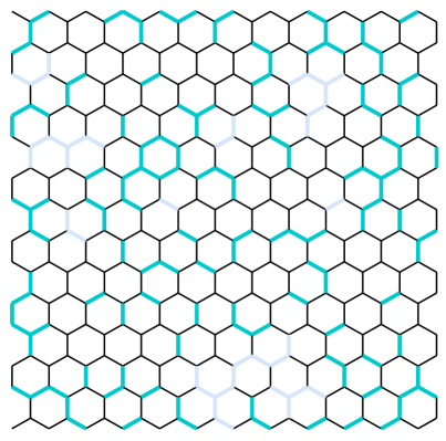
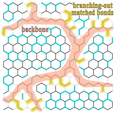
Figure 2: (Left) Illustrated is a typical distribution of matched bonds depicted as thicker (dark-cyan and light-purple) bonds. Here the bond is called matched when the pair of neighboring sites is assigned to the same axis through the polarizing measurement at the first stage of the protocol. The region to simulate a quantum circuit by the complementary bases, called the backbone, is going to be chosen by classical side-computation, so as to guarantee its global topology is identical to that of the target quantum circuit (cf. the Section 5). To this end, the backbone must skirt some “off-limits” configurations of matched-bond clusters that induce additional undesirable logical loops if all of them are involved in the backbone. Accordingly, it is sufficient that every quantum logical wire is chosen from any horizontally percolating path that circumvents only some clusters of matched bonds, for instance, colored in light purple. (Right) A possible embedding of the backbone, described as a shaded pinkish-orange region, has been identified by analyzing classically the occurrence of matched bonds . The “branching-out” matched bonds that are involved in the backbone and described by a shaded yellow region are the extended region where the logical information of quantum computation is processed in the second stage of the protocol. However, by having no additional closed loop, they would not disturb the desired logical action. Based on the statistical property originated from the genuine 2D nature of correlations of the AKLT state, the almost sure success of such an identification of the suitable backbone is guaranteed in an analogous way with the emergence of the macroscopic percolating cluster in the bond percolation phenomenon. The microscopic view near the CNOT gate is highlighted in the Figure 1.

A key insight to construct our protocol is that since the reduced density operator of every spin $\tfrac{3}{2}$ per site is totally mixed and isotropic, i.e., the normalized identity projector $\tfrac{{\bf 1}}{4}$, we are able to extract 2 bits of classical information by measurements per site. Then it is sensible that in stead of obtaining them at once, a part of the information, indeed $\log_{2}3$ bits in our case, is first extracted and we adapt the next stage according to it. It might be surprising that the first measurement induces a kind of randomization, but intuitively speaking, this part is crucial to separate the original quantum correlation that intrinsically involves genuine 2D fluctuations into the classical correlation (or, a statistical sampling) that can be still efficiently handled by a classical side-processor and the “more rigid” quantum correlation suitable for deterministic quantum computation. A global statistical nature of the AKLT correlations through the first stage guarantees, in an analogous way with the classical percolation phenomenon, that an embedding of the backbone (i.e. the target quantum circuit) can be found in the typical configuration of a heralded, randomized distribution of entanglement. At the second stage which implements quantum computation, the protocol is invented in such a way that the standard-basis measurement and complementary-basis one, both of which are defined later, are paired (as depicted by the dotted bonds in the Figure 1). This paired processing is crucial to make the logical information bound in the domain of the backbone, somehow in a reminiscent way how the deoxyribonucleic acid (DNA) holds genetic information in its famous double strands.

Summary of the MQC protocol

Now we outline our MQC protocol, which consists of two stages. (i) The first stage is to apply a measurement $\{M^{x},M^{y},M^{z}\}$ which polarizes randomly toward one of the three orthogonal axes at every site. We define a degenerate projection $M^{\mu}\;(\mu=x,y,z)$ as

$$M^{\mu}=\sqrt{\tfrac{2}{3}}(|\tfrac{3}{2}^{\mu}\rangle\langle\tfrac{3}{2}^{\mu}|+|-\tfrac{3}{2}^{\mu}\rangle\langle-\tfrac{3}{2}^{\mu}|).$$ (6)

The set of $\{M^{x},M^{y},M^{z}\}$ constitutes the positive operator value measure (POVM) by satisfying $\sum_{\mu=x,y,z}M^{\mu\dagger}M^{\mu}={\bf 1}$, so that it is a valid local measurement with three alternative, random outcomes $\mu$. We must record the outcome $\mu_{k}$ at every site $k$ and collect the location of such matched bonds that the pair of the axes for the neighboring sites $k,k^{\prime}$ coincides, namely $\mu_{k}=\mu_{k^{\prime}}$ . Based on the occurrence of matched bonds (which need additional care in their use), we are able to determine the backbone by efficient classical side-computation in circumventing some rare “off-limits” configurations of matched bonds defined later.

(ii) The second stage carries actual quantum computation, using further projective measurements at every site and feedforward of their outcomes. Once the backbone is identified, the computation is deterministic in a very similar way with MQC on the 2D cluster state.

4 Widgets for the logical gates

A basic idea of the widgets to construct the logical gates from the set of tensors is outlined first. Suppose the bond is not matched for a pair of the nearest neighboring sites, then either of the sites can be used as the part of the backbone, by treating the other as the non-backbone site. Let the assignment of the first-stage polarizing measurement at the backbone site be $\mu$ and the other be $\nu(\neq\mu)$, and, as an illustration, assume $\mu=z$ at the $\top$ site and $\nu=x$ at the $\bot$ site. It turns out that, in measuring the non-backbone site in the basis of $\{\left\langle\tfrac{3}{2}^{x}\right|,\left\langle-\tfrac{3}{2}^{x}\right|\}$ (since the state is already in this subspace by the preceding $M^{x}$), we can always get a unitary action at the backbone site along the other remaining two bonds, regardless of which outcome has occurred. This is because conditioned on the specification of the tensor of Eqs. (4,5) to be, for instance, $|0^{x}\rangle\langle 1^{x}|\otimes\left|0^{x}\right\rangle$ by the outcome $\left\langle\tfrac{3}{2}^{x}\right|$ at the non-backbone site, the tensors at the backbone site are essentially fixed as

$$\begin{split}\tilde{A}_{\top}[\tfrac{3}{2}^{z}]&=|0^{z}\rangle\langle 1^{z}|\otimes\langle 1^{z}|0^{x}\rangle=\tfrac{1}{\sqrt{2}}|0^{z}\rangle\langle 1^{z}|,\\ \tilde{A}_{\top}[-\tfrac{3}{2}^{z}]&=|1^{z}\rangle\langle 0^{z}|\otimes\langle 0^{z}|0^{x}\rangle=\tfrac{1}{\sqrt{2}}|1^{z}\rangle\langle 0^{z}|.\end{split}$$ (7)

The overall numerical factor $\tfrac{1}{\sqrt{2}}$ implies the fact that the outcome $\left\langle\tfrac{3}{2}^{z}\right|$ would occur with probability $\tfrac{1}{2}$, and of course the other outcome would do with the same probability $\tfrac{1}{2}$. Indeed, the measurements used for the unitary actions are unbiased in their output probability. Here after, however, we do not describe the overall factor explicitly, since it is irrelevant to the statistics of the logical output of quantum computation. It can be readily seen that we can get a unitary gate by mixing these two tensors in such a way that for instance, measuring this backbone site in the basis $\{\tfrac{1}{\sqrt{2}}(\left\langle\tfrac{3}{2}^{z}\right|+\left\langle-\tfrac{3}{2}^{z}\right|),\tfrac{1}{\sqrt{2}}(-\left\langle\tfrac{3}{2}^{z}\right|+\left\langle-\tfrac{3}{2}^{z}\right|)\}$ provides $X(=\tilde{A}_{\top}[\tfrac{3}{2}^{z}]+\tilde{A}_{\top}[-\tfrac{3}{2}^{z}])$ or $XZ(=-\tilde{A}_{\top}[\tfrac{3}{2}^{z}]+\tilde{A}_{\top}[-\tfrac{3}{2}^{z}])$ respectively. Both unitary actions should be interpreted as the logical identity since the difference by a Pauli operator can be readily incorporated, as explained later, by the adaptation of the following measurement basis so that the Pauli operators are treated as the byproduct operator $\Upsilon$. In more general, measuring in a basis on the plane spanned by the aforementioned two vectors is found to provide the logical rotation $R^{z}(\theta)=|0^{z}\rangle\langle 0^{z}|+e^{i\theta}|1^{z}\rangle\langle 1^{z}|$ by an arbitrary angle $\theta$ along the axis $z$. We call any of such bases complementary to the standard basis $\{\left\langle\tfrac{3}{2}^{\mu}\right|,\left\langle-\frac{3}{2}^{\mu}\right|\}$ given the axis $\mu$ at the site. The choice of the complementary basis depends on the axis $\nu$ of the associated non-backbone site. Accordingly, we may denote the complementary basis in an abstract way as $\{\left\langle\gamma^{\mu|\nu}\right|\}$, which will be explicitly defined later.

Such a construction of a “mutually-unbiased” input to the backbone is the key technique provided by the pair of the standard-basis and complementary-basis measurements. Indeed, this basic idea is shown to be extensible with an additional care even when the bond is matched. As it will get clearer, the set of sites measured in the complementary bases, which covers strictly the backbone, corresponds to the region where logical information of quantum computation is processed. Our construction enables us to decouple the logical output probability of quantum computation from the rest of the sites measured in the standard-basis measurements (conditioned on the configuration of the axis per site after the first stage of the protocol). A suitable identification of the backbone is addressed later in the Section 5 as a global nature of computational capability, supported by a prescription to the matched bonds in the B.

4.1 Single-qubit logical gates

Any single-qubit logical gate in $SU(2)$ can be implemented by the sequence of the rotations $R^{\mu}(\theta)=|0^{\mu}\rangle\langle 0^{\mu}|+e^{i\theta}|1^{\mu}\rangle\langle 1^{\mu}|$ along two independent axes, using the Euler angles $\theta$’s. Here we take $\mu=z$ and $x$ without loss of generality, and describe the detailed protocol for $R^{z}(\theta)$.

The $R^{z}(\theta)$ can be only attempted if the axis $\mu$ of the backbone site is assigned to be $z$ after the polarizing measurement at the first stage. Otherwise we teleport the logical information along the backbone by implementing the logical identity by measuring the site in the complementary basis with the fiducial angle (i.e., $\theta=0$) until we reach the backbone site with $\mu=z$. Let the axis of the associated non-backbone site be $\nu$, and the outcome when measured in the standard basis denoted as $c\in\{0,1\}$ in corresponding to $\left\langle(-1)^{c}\tfrac{3}{2}^{\nu}\right|$. The complementary basis for the given axis $\mu=z$ is defined (at both the $\top$ and $\bot$ sites) as, if $\nu=x$,

$$\langle\gamma^{z|x}(\theta)|=\tfrac{1}{2\sqrt{2}}\left[(1+(-1)^{b}e^{i\theta})\left(\left\langle\tfrac{3}{2}^{z}\right|+\left\langle-\tfrac{3}{2}^{z}\right|\right)+(1-(-1)^{b}e^{i\theta})\left(-\left\langle\tfrac{3}{2}^{z}\right|+\left\langle-\tfrac{3}{2}^{z}\right|\right)\right],$$ (8)

where $b\in\{0,1\}$ corresponds to each outcome of the orthogonal projective measurement with the angle $\theta$ or $\theta+\pi$ respectively, and if $\nu=y$,

$$\langle\gamma^{z|y}(\theta)|=\tfrac{1}{2\sqrt{2}}\left[(1+(-1)^{b}e^{i\theta})\left(-i\left\langle\tfrac{3}{2}^{z}\right|+\left\langle-\tfrac{3}{2}^{z}\right|\right)+(1-(-1)^{b}e^{i\theta})\left(i\left\langle\tfrac{3}{2}^{z}\right|+\left\langle-\tfrac{3}{2}^{z}\right|\right)\right].$$ (9)

In all the cases, the logical action is given by

$$\sum_{\alpha}\tilde{A}[\alpha]\langle\gamma^{z|\nu}(\theta)|M^{z}|\alpha\rangle=XZ^{b\oplus c}R^{z}(\theta),$$ (10)

where a partial contraction has been made, in the same way as in Eq. (7), with the rank-1 tensor from the associated non-backbone site, using the notation

$$\tilde{A}_{\top}[\alpha]=A_{\top}[\alpha]\left|c^{\nu}\right\rangle,\quad\tilde{A}_{\bot}[\alpha]=\left\langle c\oplus 1^{\nu}\right|A_{\bot}[\alpha].$$ (11)

This is the desired rotation up to a Pauli byproduct $\Upsilon=XZ^{b\oplus c}$. Note that the choice of the various complementary bases only depends on the axis $\nu$ and not on the outcome $c$ at the non-backbone site, so that once the axis of every site has been assigned and the backbone structure has been determined, the backbone site and its associated non-backbone site can be measured in a parallel way. Likewise, the counterpart for $R^{x}(\theta)$ can be obtained by

$$\langle\gamma^{x|z}(\theta)|=\tfrac{1}{2\sqrt{2}}\left[(1+(-1)^{b}e^{i\theta})\left(\left\langle\tfrac{3}{2}^{x}\right|+\left\langle-\tfrac{3}{2}^{x}\right|\right)+(1-(-1)^{b}e^{i\theta})\left(-\left\langle\tfrac{3}{2}^{x}\right|+\left\langle-\tfrac{3}{2}^{x}\right|\right)\right],$$ (12)

$$\langle\gamma^{x|y}(\theta)|=\tfrac{1}{2\sqrt{2}}\left[(1+(-1)^{b}e^{i\theta})\left(i\left\langle\tfrac{3}{2}^{x}\right|+\left\langle-\tfrac{3}{2}^{x}\right|\right)+(1-(-1)^{b}e^{i\theta})\left(-i\left\langle\tfrac{3}{2}^{x}\right|+\left\langle-\tfrac{3}{2}^{x}\right|\right)\right].$$ (13)

The measurement in these complementary bases result in $\Upsilon R^{x}(\theta)$ with $\Upsilon=ZX^{b\oplus c}$. Although it is straightforward to define $\left\langle\gamma^{y|\nu}(\theta)\right|$ for $R^{y}(\theta)$, it is theoretically sufficient that the sites labelled by $\mu=y$ are only used for the logical identity (with $\theta=0$), whose dependence to the outcomes is $\Upsilon=X^{b\oplus c}Z^{b\oplus c\oplus 1}$. The dependence of the byproduct operator $\Upsilon$ on measurement outcomes is summarized in the Table 1.

In the above, we have assumed that the (degree-2) backbone site has in tow its neighboring non-backbone site which is measured in the standard basis along $\nu$ and provides the outcome $c$. If the backbone site is connected via the matched bonds to its associated non-backbone site, then the intermediate sites should be measured in the complementary basis too, and a correction to $\left|c^{\nu}\right\rangle$ (or $\left\langle c\oplus 1^{\nu}\right|$) of $\tilde{A}[\alpha]$ defined by Eq. (11) is required. Roughly speaking, the non-backbone sites connected by the “branching-out” matched bonds (colored in yellow in the Figure 2) need to be treated in the same way as the backbone sites, so that we have to sum up all their byproduct operators. The motivation as well as technical detail of this prescription to the matched bonds is found in the B.

$\mu$	$a^{x}$	$a^{z}$
$\gamma^{x|\nu}$	$b\oplus c$	1
$\gamma^{y|\nu}$	$b\oplus c$	$b\oplus c\oplus 1$
$\gamma^{z|\nu}$	1	$b\oplus c$

Table 1: The indices $(a^{x},a^{z})$ of the byproduct operator $\Upsilon=X^{a^{x}}Z^{a^{z}}$ for the complementary basis measurement $\{\langle\gamma^{\mu|\nu}|\}$ given the axis $\mu$, where $b$ is the outcome of the site measured in this basis, and $c$ is the outcome of the associated site (connected to the former directly by an unmatched bond) measured in the standard basis of the axis $\nu$ .

4.2 Two-qubit logical gate: CNOT

Together with the arbitrary single-qubit logical gates on every logical wire, it is widely known that any entangling two-qubit logical gate is sufficient to achieve the universality of quantum computation when the quantum circuit is composed from the set of these gates. Here we take the target two-qubit logical gate to be the controlled-not (CNOT) gate, $|0^{z}\rangle\langle 0^{z}|\otimes{\bf 1}+|1^{z}\rangle\langle 1^{z}|\otimes X$.

The two-qubit logical gate requires connecting a pair of the degree-3 backbone sites with the $\top$ and $\bot$ bonds for each. In particular, the CNOT uses the degree-3 $\top$ site with the axis $\mu_{1}=z$ and the degree-3 $\bot$ site with $\mu_{2}=x$. One could in principle use a matched-bond cluster with the same axis, instead of the single degree-3 site. Observe that

$$\begin{split}A_{\top}[\gamma^{z|x}(0)]&=\tfrac{1}{\sqrt{2}}\Upsilon_{\top}\left({\bf 1}\otimes\left\langle 0^{x}\right|+Z\otimes\left\langle 1^{x}\right|\right),\\ A_{\bot}[\gamma^{x|z}(0)]&=\tfrac{1}{\sqrt{2}}\Upsilon_{\bot}\left({\bf 1}\otimes\left|0^{z}\right\rangle+X\otimes\left|1^{z}\right\rangle\right),\end{split}$$ (14)

where the byproducts are $\Upsilon_{\top}=XZ^{b_{\top}}\otimes{\bf 1}$ and $\Upsilon_{\bot}=X^{b_{\bot}\oplus 1}Z\otimes Z$, and the conditioning axes $\nu_{1},\nu_{2}$ of the complementary bases can be chosen freely, so that we have set $\nu_{1}=x$ and $\nu_{2}=z$ for convenience. So, when the vertical direction (the second degree of freedom in the tensor structure of Eq. (14)) is contracted through the sequence of the logical identities in the same way as in the part of a quantum logical wire, it is readily seen that this provides the desired CNOT $(=\tfrac{1}{2}\left({\bf 1}\otimes{\bf 1}+{\bf 1}\otimes X+Z\otimes{\bf 1}-Z\otimes X\right))$.

Here we need to calculate the total byproduct operator from this intermediate vertical part, namely $\Upsilon_{|}=X^{\sum_{k}a^{x}_{k}}Z^{\sum_{k}a^{z}_{k}}$ where the summation is taken over the degree-2 backbone sites symbolically labeled by $k$. Needless to say, if there are, in between, the branches by the matched bonds, we have to take their contribution into account according to the prescription of the B, in order to determine $(a^{x}_{k},a^{z}_{k})$ at every junction to the branch. Thus, $\Upsilon_{|}$ essentially amounts to the whole accumulation of the byproducts from the vertical part. By absorbing $Z^{\sum_{k}a^{z}_{k}\oplus 1}$ (which has included the additional one from $\Upsilon_{\bot}$) into $\left\langle 0/1^{x}\right|$ of $A_{\top}$, as well as $X^{\sum_{k}a^{x}_{k}}$ into $\left|0/1^{z}\right\rangle$ of $A_{\bot}$, we can reduce them to the byproduct operators along two logical wires. The whole logical action is $\Upsilon{\rm CNOT}$, where $\Upsilon=XZ^{b_{\top}\oplus\sum_{k}a^{z}_{k}\oplus 1}\otimes X^{b_{\bot}\oplus\sum_{k}a^{x}_{k}\oplus 1}Z$.

4.3 Initialization and readout

The initialization and readout (in the sense of the quantum circuit model) of the logical wire can be simulated as well. Suppose, without loss of generality, these are always made in the $\left|0/1^{z}\right\rangle$ basis. All we have to do is to find the degree-2 backbone site with $\mu=z$ on the rightmost (for the initialization) and on the leftmost (for the readout) of every logical wire, and to measure it in the standard basis $\{\left\langle\tfrac{3}{2}^{z}\right|,\left\langle-\tfrac{3}{2}^{z}\right|\}$. As already described through the notation for the standard-basis measurement, according to Eqs. (3, 4), the outcome $c$ must be interpreted as $\left|c^{z}\right\rangle$ or $\left\langle c\oplus 1^{z}\right|$. Note, in particular regarding the readout, that the outcome $c$ at the leftmost boundary site is not immediately the logical outcome of the computation. The latter is evaluated only together with the byproduct operator at the end of the computation.

4.4 Adaptation based on byproduct operators

Since the byproduct operator $\Upsilon$ stays in the Pauli group, we can use the same machinery as the cluster-state MQC, to deal with the randomness of the measurement outcome. The key idea is to postpone the effect of $\Upsilon$ by adapting the following angles of the logical rotations. As an illustration, suppose we wish to apply the sequence of $R^{z}(\theta^{z})$ followed by $R^{x}(\theta^{x})$ up to some byproduct operator $\Upsilon$, namely $\Upsilon R^{x}(\theta^{x})R^{z}(\theta^{z})$. Since

$$(X^{b^{\prime}\oplus c^{\prime}}ZR^{x}(\theta^{x}))(XZ^{b\oplus c}R^{z}(\theta^{z}))=X^{b^{\prime}\oplus c^{\prime}\oplus 1}Z^{b\oplus c\oplus 1}R^{x}((-1)^{b\oplus c}\theta^{x})R^{z}(\theta^{z}),$$ (15)

we realize that if we adapt the second angle $\theta^{x}$ to be $(-1)^{a^{z}}\theta^{x}$, based on the byproduct index $a^{z}=b\oplus c$ of the first measurement, we can always apply the desired sequence of the rotations regardless of the outcomes $b$ and $c$. In general, we have to adapt the angle of the next logical rotation, based on the current byproduct operator $\Upsilon$ updated according to the simulated time direction of the quantum circuit. Note that such an adaptation is required only if the rotation angle is not fiducial, so that the part by the logical identities does not need the adaption and can be implemented parallely in principle. Since this adaptation is now a widely-known machinery in MQC, we leave the details to the literatures, e.g., Ref. [7] (although in the case of the cluster state there is an additional automatic logical operation by the Hadamard matrix $\tfrac{1}{\sqrt{2}}(X+Z)$ at every single step of computation).

5 Global nature of emergent computational capability

5.1 Identification of the backbone

In this section, we show that the backbone structure, which should be intact from rare “off-limits” configurations of matched bonds, can be identified efficiently in analyzing their occurrence by classical side-computation. The analysis not only guarantees that the widgets for the logical gates in the Section 4 can be composed consistently, but also suggests how the computational capability as a whole is linked to the emergence of a macroscopic feature of the many-body system.

Recall that, at the first stage of the protocol, every outcome of the polarizing measurement $\{M^{\mu}\}\;(\mu=x,y,z)$ occurs randomly at every site, i.e., with the equal probability $\tfrac{1}{3}$. Thus, in neglecting two-point correlation functions exponentially decaying in distance as a first approximation, we can imagine that the bond between a pair of the neighboring sites is unmatched with probability $\tfrac{2}{3}$ and matched with probability $\tfrac{1}{3}$. Indeed, the effect of two-point correlations is very limited, and it seems to modify the probability of the unmatched bond by not more than 1 percent. Accordingly, we could visualize in our mind a typical configuration of unmatched bonds, as presented in the Figure 2, by the proximity to the bond percolation model with an occupation probability $p=\tfrac{2}{3}$. As a reference, it is widely known in the bond percolation model that, when $p$ is larger than the critical value $p_{c}=1-2\sin(\tfrac{\pi}{18})\approx 0.652\ldots$ [23] for the 2D hexagonal lattice, there exists almost surely (i.e., with a probability close to the unity exponentially in the lattice size) a single macroscopic cluster of the occupied bonds, spanning the whole lattice.

Importantly, it is shown (in detail in the B) that not only unmatched bonds, which are the majority, but also most of matched bonds are indeed available as a part of the backbone under our prescription. The key idea is a “topological encoding” of the backbone structure in that in most cases the matched-bond cluster touching the backbone and measured in its complementary basis can be made to constitute a micro-circuit whose output to the backbone is mutually-unbiased as if the whole cluster were a single unmatched bond. In other words, the matched-bond cluster can be effectively renormalized to the single logical site directly on the backbone (which is called the “root” site in the B), regardless of the size and shape of the cluster. This prescription clarifies that the backbone should be identified in order that the region measured in the complementary bases (namely, the backbone and all the matched-bond cluster touching it) does not induce any additional closed loop which is absent in the target quantum circuit.

For a practical algorithmic implementation, we could leverage a variety of polynomial-time classical algorithms (see e.g., Ref. [24]) developed through the study of percolation models. For instance, using an existing method to detect the locations of matched-bond clusters locally from the records of the polarizing measurement outcome at every site, we can efficiently mark potential off-limits configurations that two matched-bond clusters with different axes are nearest neighboring via more than one unmatched bond (see the B for their precise notion related to the existence of closed loops). This is because measuring both clusters in complementary bases must result in an undesired closed loop inevitably. So, one could consider one of such clusters to be effectively “unoccupied” bonds (which are marked by thicker, light-purple bonds in the Figure 2), and choose the backbone from the remaining (unmatched and matched) bonds.

Thus, our situation is much more favorable to find every horizontally percolating path corresponding to a quantum logical wire, compared to the case where such a path should be found from the cluster of unmatched bonds only. The ratio of “occupied” bonds is much larger than $\tfrac{2}{3}$ effectively, and our macroscopic cluster of the occupied bonds can indeed offer abundant choices. For this purpose, it is straightforward to apply to our context the same efficient classical algorithm to find multiple percolating paths, despite that the unoccupied bonds are not generated according to the standard percolation model. That may involve, in practice, some customization such as a preference to the sites with certain axes (depending on the choice of the elementary gates) and optimization about physical overheads, but we do not intend to pursue concrete algorithms further. Note that the use of a percolation phenomenon has been previously considered in the context of MQC but in rather different scenarios [25, 26] where the preparation of a cluster state suffers some locally probabilistic errors. For example, Ref. [26] has presented a detailed algorithm to extract explicitly multiple percolating paths for a 2D cluster state. Such machinery to the cluster state is also used in another approach to indicate computational usefulness of the 2D AKLT state in Ref. [19].

Only a practically notable constraint by the matched bonds is on the spatial overhead of the backbone, in particular, the spacing between every neighboring pair of quantum logical wires running horizontally. Two quantum logical wires are not supposed to enter a single matched-bond cluster, since the latter behaves as the single logical site effectively. According to the approximation by the percolation model, it is expected that the size of the largest matched-bond cluster scales logarithmically in the lattice size but it occurs with an exponentially small probability. Since we would likely resort to quantum error correction to the goal of a scalable fault-torelant quantum computer in the end, we can set a cutoff within its constant error threshold, so as to disregard the rare large clusters and to deal with them in the similar way with other errors. It means that a constant spacing between two neighboring logical wires would be sufficient.

5.2 Emergence of a simulated space-time

It is remarkable to see how the distinction between (simulated) space and time emerges in our model. Our backbone structure after the first stage does not distinguish them yet, but we can realize, by a careful examination of the protocol, it originates from the way the byproduct indices $(a^{x},a^{z})$, namely two bits of classical information processed at each site, are communicated to the neighbors. Time emerges when both two indices are forwarded in the same (and roughly horizontal here) direction, while space emerges when two are sent in the opposite (and roughly vertical here) directions as is the case of CNOT, where $a^{x}$ or $a^{z}$ is sent downward or upward, respectively. Note also that since the spatial-entangling gate, like CNOT, is simulated only using the measurements with the fiducial angle and thus need not be adapted, there is indeed no “time-ordering” along the simulated spatial direction.

6 Discussion

6.1 Ground-code MQC

A feature that our resource is available as the ground state can be leveraged during the computational process in addition to the stage of its preparation. As originally proposed in Ref. [11] as the ground-code version of MQC using coupled 1D AKLT states, if we are capable of adiabatically turning off a two-body interacting term only to the spin to be measured selectively — importantly that still does not have to create new entanglement — we could indeed make the Hamiltonian in the remaining bulk coexist without interfering the MQC protocol for quantum computation. Then, the Hamiltonian with a (conjectured) gap would be able to contribute to a passive protection of the logical information stored in the degenerate ground state, by providing some robustness against local noises, in compared to a scenario where the bulk Hamiltonian is absent.

Here we need additional care to apply the idea of the ground code to the 2D AKLT state, since it was assumed that the spin $\tfrac{3}{2}$’s are first assigned to one of three axes through the polarizing measurement before the quantum computation starts. It turns out that it is still possible for the the classical algorithms described in the Section 5 to function if the sampling of the matched bonds are made over the block of a constant number of spins near the rightmost boundary of the unmeasured bulk, without identifying the full configuration of matched bonds deep inside the bulk.

6.2 Persistence of computational capability in the VBS phase

Another significant merit to have the bulk Hamiltonian during the computation is that any ground state which belongs to the 2D VBS phase (with the rotational symmetry as is present in the AKLT Hamiltonian) is conceived to be ubiquitously useful to simulate the same quantum computation through the aforementioned adiabatic turning off of the interaction at the boundary. Its detail will be analyzed elsewhere, but such persistence of computational capability over an entire quantum phase was unveiled in Ref. [27], in examining the rotationally-invariant 1D VBS phase to which the 1D AKLT state belongs. A key of the mechanism is indeed the edge states — fractionalized degrees of freedom emergent at the boundary of the unmeasured bulk part — that are commonly present in the VBS phase and carry the logical information of quantum computation in our context. At any point within the VBS phase, the quantum correlation between the spin to which the two-body interaction has been turned off and the emergent edge state at a new boundary of the bulk would be modified to exactly that of the AKLT state, since the AKLT Hamiltonian satisfies additionally a frustration-free property (that the global ground state also minimizes every summand of the Hamiltonian) among a parameterized class of generally-frustrated Hamiltonians within the phase. That is how the primitive of the ground-code MQC, the adiabatic turning off of the interaction followed by the measurement of the freed spin, can ubiquitously unlock computational capability persistent over the VBS phase.

In contrast, suppose our ability of the selective control of a single spin at the boundary is further limited only to its measurement and the bulk Hamiltonian is neither engineered nor present during the computational process. We may still consider implementing physically (namely probabilistically in compensation with a longer distance scale) a quantum computational renormalization, through which the correlation within the VBS phase is modified into that of a fixed point. This is envisioned based on Ref. [28] where a protocol within the 1D VBS phase was constructed so as to set the AKLT point as its fixed point. An attempt to construct a 2D counterpart of the protocol may face the intrinsic difficulty for the traditional computer to analyze correlations in the 2D system, but recent various developments of the classical methods (cf. in Refs. [29, 30, 31, 32]) regarding the renormalization of 2D entanglement might be applicable to our context.

6.3 Outlook towards physical implementations

The persistence of such computational capability over the 2D VBS phase would be encouraging towards physical implementations of our scheme. Then a fine tuning to engineer a set of specific interaction strengths in the 2D AKLT Hamiltonian of Eq. (1) may not be necessary as far as the system can be set within the “quantum computational” phase in maintaining some key symmetries such as the rotational symmetry.

The biggest difference from the 1D case is the fact that the ordinary Heisenberg point (i.e. the ground state of the Hamiltonian without biquadratic and bicubic terms in Eq. (1)) has been known to be Néel ordered [4] and does not belong to the 2D VBS phase unfortunately, although the 1D Heisenberg point is located within the 1D VBS phase. That implies that we may need a more elaborated interaction than the simplest Heisenberg interaction or a use of geometrically frustrated quantum magnets, in order to set a ground state in the 2D VBS phase. In fact, the 1D VBS phase has been identified experimentally in several natural chemical compounds such as CsNiCl₃, Y₂BaNiO₅, and so-called NENP. The 2D VBS phase seems to be less studied both theoretically and experimentally, compared to other kinds of 2D VBC phases for now. A recent discovery of the absence of spontaneous magnetic ordering in the manganese oxide Bi₃Mn₄O₁₂(NO₃) [33], which materializes an antiferromagnet of spin $\tfrac{3}{2}$’s in terms of Mn⁴⁺ ions on the 2D hexagonal lattice, might pave the way towards this direction (e.g., Ref. [34]).

Another possible realization of the 2D VBS phase is based on analog engineering of the Hamiltonians of spin lattice systems. A recent experimental development of quantum simulators in atomic, molecular, and optical physics is promising in that Mott insulating phases of ultracold Fermi spinor gases with a hyperfine manifold $F=\tfrac{3}{2}$, e.g., in terms of ⁶Li or ¹³²Cs atoms trapped in the optical lattice, might be used to simulate the 2D AKLT Hamiltonian of spin $\tfrac{3}{2}$’s along an extension of the approach in Ref. [35] for example.

Acknowledgments

I acknowledge various relevant discussions, over a long period of the project, with I. Affleck, S.D. Bartlett, G.K. Brennen, H.J. Briegel, J.-M. Cai, W. Dür, D. Gross, M.B. Hastings, H. Katsura, R. Raussendorf, J.M. Renes, A. Sanpera, N. Schuch, and T.-C. Wei. The work is supported by the Government of Canada through Industry Canada and by Ontario-MRI.

Appendix A Boundary tensor in the 2D VBS state

The boundary tensor $B$ is defined as $B=\prod_{\ell}\Upsilon_{\ell}$, where $\ell$ represents a nonlocal degree of freedom associated with every pair of the boundary sites which are supposed to be closed under the periodic boundary condition, and thus $2|\ell|$ represents the total number of the boundary sites. This term formally provides the $4^{|\ell|}$-fold initial degeneracy to the ground state, but it turns out that any of such ground states (and actually even the mixed state by them through an argument similar to Ref. [27]) is useful to our goal, because of the decoupling property to the backbone. Thus, here we set $B$ to be the identity for simplicity.

Appendix B Renormalizing prescription to matched bonds

We elaborate a technical prescription for matched bonds, and prove the following informal lemma.

Lemma.

The backbone is freely chosen as far as the global topology of the region measured in the complementary bases (namely, the backbone and all the matched-bond clusters touching to it) is equivalent to the target quantum circuit, regarding the configuration of closed loops.

The lemma can be also seen as our resolution to the genuine 2D fluctuations present in naturally-occurring systems. They are dealt, by adjusting the encoding of each single logical site to be variable according to the size and shape of every matched-bond cluster.

B.1 1D-like chain

Let us consider first a 1D-like chain of the matched bonds, branching out from a degree-2 site on the backbone of the axis $\mu$. Here we call such a site as the root site of the matched-bond cluster. The sequence does not bifurcate further, and thus is expected to terminate in the end at a non-backbone site after a chain of matched bonds. Let us for now label these sites along the matched-bond chain by $k$. As said, all the non-backbone sites along the chain of the matched bonds are measured in the complementary bases $\{\left\langle\gamma^{\mu|\nu_{k}}\right|\}$, which depend on the axis $\nu_{k}$ of each associated site connected by the unmatched bond in the third direction orthogonal to the matched-bond chain. At the end of the matched-bond chain, the terminating site must have two unmatched bonds, and its two associated sites are measured in the standard basis of each. That provides a pair $\left|c^{\nu}\right\rangle$ and $|c^{\prime\nu^{\prime}}\rangle$ to the tensors at the terminating site, so that either one, here $|c^{\prime\nu^{\prime}}\rangle$, can be used to assign $\tilde{A}[\alpha]$ to the terminating site as usual, and the other $\left|c^{\nu}\right\rangle$ plays a role of the “initial” condition to the matched-bond chain. In the exactly same way as the chain of the degree-2 backbone sites, this matched-bond chain behaves as the sequence of the logical identities acting on the initial state $\left|c^{\nu}\right\rangle$. At the root site to the backbone, the total logical effect is equivalent to input $\left|\bar{c}^{\bar{\nu}}\right\rangle$ given by

$$\left|\bar{c}^{\bar{\nu}}\right\rangle=\!\!\prod_{k}^{\rm matched}\!\!\tilde{A}_{k}[\gamma^{\mu|{\nu_{k}}}(0)]|c^{\nu}\rangle=X^{\sum_{k}a^{x}_{k}}Z^{\sum_{k}a^{z}_{k}}|c^{\nu}\rangle,$$ (16)

where $\bar{\nu}=\nu$ and

$$\bar{c}=\left\{\begin{array}[]{ll}c\oplus\sum_{k}a^{z}_{k}&\mbox{if}\;\;\nu=x,\\ c\oplus\sum_{k}(a^{x}_{k}\oplus a^{z}_{k})&\mbox{if}\;\;\nu=y,\\ c\oplus\sum_{k}a^{x}_{k}&\mbox{if}\;\;\nu=z.\end{array}\right.$$ (17)

The indices $(a^{x}_{k},a^{z}_{k})$ of the byproduct operator at every site $k$, measured in the complementary basis along the matched-bond chain, are determined according to the rule at the Table 1 (in incorporating the contributions from associated sites measured in the standard basis). $\left\langle\bar{c}\oplus 1^{\bar{\nu}}\right|$ is determined exactly in the same formula. The key observation is that the matched-bond chain all measured in the complementary basis provides a “mutually-unbiased” input state in an axis $\nu$ different from the axis $\mu$ of the matched bonds, and thus can play a comparable role to a single unmatched bond.

B.2 Locally tree structure

In general, the branching-out cluster of the matched bonds may have bifurcations like a tree locally. Flowing backward from every leaf of the tree (or, the terminating site of a matched-bond chain) according to the aforementioned procedure, we can prepare the mutually-unbiased input at each bifurcation site. Thus, we concatenate this procedure several times until it reaches the root site of the matched-bond cluster located on the backbone.

B.3 Closed loop

For completeness, we remark that closed loops may exist within the matched-bond cluster, branching out from the backbone. It essentially corresponds to the counterpart of Eq. (16) in a closed boundary condition. Suppose a closed loop, for example a hexagon, exists when we are applying the aforementioned procedure from every leaf of the cluster. Each site in the closed loop, except the the one which is closest to the root site of the cluster and called as the zeroth here, is now assumed to be associated effectively with the mutually-unbiased input using either an unmatched bond or our prescription for matched bonds. Then, the contribution by the closed loop is

$${\rm tr}_{\rm\,loop}\left[A_{0}[\gamma^{\mu|{\nu_{0}}}(0)]\!\!\prod_{k}^{\rm matched}\!\!\tilde{A}_{k}[\gamma^{\mu|{\nu_{k}}}(0)]\right],$$ (18)

where the axis $\nu_{0}$ can be chosen to be either axis different from $\mu$, and note that $A_{0}$ is the original, three-directional tensor. For example, if $\mu=z$ and the zeroth is a $\top$ site, Eq. (18) is equivalent to

$$\sum_{\bar{c}=0,1}{\rm tr}\left[X^{1\oplus\sum_{k}a^{x}_{k}}Z^{b_{0}\oplus\bar{c}\oplus 1\oplus\sum_{k}a^{z}_{k}}\right]\otimes\left\langle\bar{c}\oplus 1^{\nu_{0}}\right|,$$ (19)

by denoting the zeroth-site bare outcome as $b_{0}$. Remarkably, careful examination of the Table 1 clarifies that the total byproduct operator along the loop could accumulate up to the identity operator (with a regular weight $\tfrac{1}{\sqrt{2}}$), and the contribution of Eq. (18) is always non-vanishing. In this example, $1\oplus\sum_{k}a^{x}_{k}\equiv 0$ because the number of sites constituting a loop must be even and every $a^{x}_{k}$ is always $1$ according to the Table 1. Thus, the closed loop of matched bonds provides likewise a mutually-unbiased input $\left|\bar{c}^{\bar{\nu}}\right\rangle$ or $\left\langle\bar{c}\oplus 1^{\bar{\nu}}\right|$ towards the root site, where $\bar{\nu}=\nu_{0}$ and

$$\bar{c}\oplus 1=\left\{\begin{array}[]{ll}b_{0}\oplus\sum_{k}a^{x}_{k}&\mbox{if}\;\;\mu=x,\\ b_{0}\oplus\sum_{k}a^{x}_{k}=b_{0}\oplus\sum_{k}(a^{z}_{k}\oplus 1)&\mbox{if}\;\;\mu=y,\\ b_{0}\oplus\sum_{k}a^{z}_{k}&\mbox{if}\;\;\mu=z,\end{array}\right.$$ (20)

in analogy to Eq. (17).

This analysis suggests that the closed loop itself can be directly a part of the backbone, namely can share one or more bonds with the backbone. Phrased differently, the matched-bond loop (of the same axis) does not disturb the global topology of the backbone. This can be confirmed by inserting, instead of $A_{0}$, two original three-directional tensors, e.g. $A_{\rm in}$ and $A_{\rm out}$ at a $\top$ and a $\bot$ site respectively with $\mu=z$ and $\nu_{0}=x$ or $y$, in Eq. (18). Note that the two are not necessarily the nearest neighbors, nor necessarily $\top$ and $\bot$ sites in general.

$${\rm tr}_{\rm\,loop}\left[A_{\rm out}[\gamma^{z|{\nu_{0}}}(0)]\!\!\prod_{k}^{\rm matched}\!\!\tilde{A}_{k}[\gamma^{z|{\nu_{k}}}(0)]A_{\rm in}[\gamma^{z|{\nu_{0}}}(0)]\right]$$

$$=\sum_{c,c^{\prime}=0,1}\!\!{\rm tr}\left[X^{2\oplus\sum_{k}a^{x}_{k}}Z^{b_{\bot}\oplus c^{\prime}\oplus\sum_{k}a^{z}_{k}\oplus b_{\top}\oplus c}\right]\otimes|{c^{\prime}}^{\nu_{0}}\rangle\left\langle c\oplus 1^{\nu_{0}}\right|=Z^{b_{\top}\oplus b_{\bot}\oplus\sum_{k}a^{z}_{k}\oplus 1},$$ (21)

where in the last equality we have used the non-vanishing condition of the trace, $c\oplus c^{\prime}=b_{\top}\oplus b_{\bot}\oplus\sum_{k}a^{z}_{k}$ (i.e., the parity of $c$ and $c^{\prime}$ is fixed), based on the property that the exponent of the Pauli $X$ operator is identically zero once again. Thus, the contribution by the loop is a power of the Pauli $\mu$ operator depending on the measurement outcomes in an extended manner of the Table 1. It is also straightforward to see that we could get further $R^{z}(\theta)$ by this matched-bond cluster, by replacing one of fiducial rotations by $\theta$, as usual.

In a nutshell, as mentioned in the main text, the cluster of matched bonds can be effectively treated as a single logical site under our renormalizing prescription, regardless of its size and shape.

B.4 Off-limits configuration

On the contrary, suppose a closed loop of sites measured in the complementary bases is introduced by a situation that the backbone touches sequentially two kinds of matched-bond clusters (with different axes, say $\mu=x$ and $z$) nearest neighboring via two or more unmatched bonds. Then the contribution of the induced loop does change the global topology of the backbone. As an illustration, suppose the induced loop consists of the matched-bond cluster of the $z$ axis and a single site of the $x$ axis, all of which are measured in their own complementary bases. By replacing in Eq. (21) the axis $z$ at $A_{\rm in}$ by $x$ (implicitly there are two unmatched bonds in the loop), we see that

$${\rm tr}_{\rm\,loop}\left[A_{\rm out}[\gamma^{z|{\nu^{\prime}_{0}}}(0)]\!\!\prod_{k}^{\rm matched}\!\!\tilde{A}_{k}[\gamma^{z|{\nu_{k}}}(0)]A_{\rm in}[\gamma^{x|{\nu_{0}}}(0)]\right]$$

$$=\sum_{c,c^{\prime}=0,1}\!\!{\rm tr}\left[X^{b_{\top}\oplus c\oplus\sum_{k}a^{x}_{k}}Z^{b_{\bot}\oplus c^{\prime}\oplus\sum_{k}a^{z}_{k}}\right]\otimes|c^{\prime\nu^{\prime}_{0}}\rangle\left\langle c\oplus 1^{\nu_{0}}\right|=|b_{\bot}\oplus\mbox{$\sum_{k}$}a^{z\,\nu^{\prime}_{0}}_{k}\rangle\left\langle b_{\top}\oplus 1^{\nu_{0}}\right|.$$ (22)

The resulting map is not unitary anymore in contrast to Eq. (21). Such an off-limits configuration would be readily circumvented through local analysis of the configuration of matched-bond clusters. In the Figure 2, we have illustrated marking (by light purple) the off-limits configurations, where each cluster is paired with another cluster in such a manner that both should not be measured in the complementary bases.

References

- [1] D.P. DiVincenzo, Fortschr. Phys. 48, 771 (2000).
- [2] R. Feynman, Int. J. Theor. Phys. 21, 467 (1982).
- [3] I. Affleck, T. Kennedy, E.H. Lieb, and H. Tasaki, Phys. Rev. Lett. 59, 799 (1987).
- [4] I. Affleck, T. Kennedy, E.H. Lieb, and H. Tasaki, Comm. Math. Phys. 115, 477 (1988).
- [5] H.J. Briegel and R. Raussendorf, Phys. Rev. Lett. 86, 910 (2001).
- [6] R. Raussendorf and H.J. Briegel, Phys. Rev. Lett. 86, 5188 (2001).
- [7] R. Raussendorf, D.E. Browne, and H.J. Briegel, Phys. Rev. A 68, 022312 (2003).
- [8] F. Verstraete and J.I. Cirac, Phys. Rev. A 70, 060302(R) (2004).
- [9] D. Gross and J. Eisert, Phys. Rev. Lett. 98, 220503 (2007).
- [10] D. Gross, J. Eisert, N. Schuch, and D. Perez-Garcia, Phys. Rev. A 76, 052315 (2007).
- [11] G.K. Brennen and A. Miyake, Phys. Rev. Lett. 101, 010502 (2008).
- [12] D. Gross and J. Eisert, Phys. Rev. A 82, 040303(R) (2010).
- [13] S.D. Bartlett and T. Rudolph, Phys. Rev. A 74, 040302(R) (2006).
- [14] T. Griffin and S.D. Bartlett, Phys. Rev. A 78, 062306 (2008).
- [15] X. Chen, B. Zeng, Z.-C. Gu, B. Yoshida, and I.L. Chuang, Phys. Rev. Lett. 102, 220501 (2009).
- [16] J.-M. Cai, A. Miyake, W. Dür, and H.J. Briegel, Phys. Rev. A 82, 052309 (2010).
- [17] M.A. Nielsen, Rep. Math. Phys. 57, 147 (2006).
- [18] M. Van den Nest, K. Luttmer, W. Dür, and H.J. Briegel, Phys. Rev. A 77, 012301 (2008)
- [19] T.-C. Wei, I. Affleck, and R. Raussendorf, Phys. Rev. Lett. 106, 070501 (2011).
- [20] D.P. Arovas, A. Auerbach, and F.D.M. Haldane, Phys. Rev. Lett. 60, 531 (1988).
- [21] T. Kennedy, E.H. Lieb, and H. Tasaki, J. Stat. Phys. 53, 383 (1988).
- [22] H. Katsura, N. Kawashima, A.N. Kirillov, V.E. Korepin, and S. Tanaka, J. Phys. A: Math. Theor. 43, 255303 (2010).
- [23] M.F. Sykes and J.W. Essam, J. Math. Phys. 5, 1117 (1964).
- [24] A.K. Hartmann and H. Rieger, “Optimization algorithms in physics,” (Wiley-VCH, Berlin, 2001).
- [25] K. Kieling, T. Rudolph, and J. Eisert, Phys. Rev. Lett. 99, 130501 (2007).
- [26] D.E. Browne, M.B. Elliott, S.T. Flammia, S.T. Merkel, A. Miyake, and A.J. Short, New J. Phys. 10, 023010 (2008).
- [27] A. Miyake, Phys. Rev. Lett. 105, 040501 (2010).
- [28] S.D. Bartlett, G.K. Brennen, A. Miyake, and J.M. Renes, Phys. Rev. Lett. 105, 110502 (2010).
- [29] G. Vidal, Phys. Rev. Lett. 101, 110501 (2008).
- [30] M. Levin and C.P. Nave, Phys. Rev. Lett. 99, 120601 (2007).
- [31] J.I. Cirac and F. Verstraete, J. Phys. A: Math. Theor. 42, 504004 (2009).
- [32] Z.-C. Gu and X.-G. Wen, Phys. Rev. B 80, 155131 (2009).
- [33] O. Smirnova, M. Azuma, N. Kumada, Y. Kusano, M. Matsuda, Y. Shimakawa, T. Takei, Y. Yonesaki, and N. Kinomura, J. Am. Chem. Soc. 131, 8313 (2009).
- [34] R. Ganesh, D.N. Sheng, Y.-J. Kim, and A. Paramekanti, Phys. Rev. B 83, 144414 (2011).
- [35] K. Eckert, Ł. Zawitkowski, M.J. Leskinen, A. Sanpera, and M. Lewenstein, New J. Phys. 9, 133 (2007).