Two-particle Kapitza-Dirac diffraction

Abstract

We extend the study of Kapitza-Dirac diffraction to the case of two-particle systems. Due to the exchange effects the shape and visibility of the two-particle detection patterns show important differences for identical and distinguishable particles. We also identify a novel quantum statistics effect present in momentum space for some values of the initial particle momenta, which is associated with different numbers of photon absorptions compatible with the final momenta.

PACS: 42.50.Xa; 03.75.Dg; 61.05.J-

1 Introduction

A long time ago Kapitza and Dirac proposed that a standing-wave light field can act as a diffraction grating [1]. This proposal is interesting in two main aspects. On the one hand, from the fundamental point of view, it provides a nice demonstration of the wave-particle duality where the diffraction grating is not massive, but made of massless entities, the photons. On the other hand, from a more practical perspective, it allows for the design of matter-wave interferometers (see, for instance, [2]). The effect has been experimentally observed, first with atomic beams [3, 4], later with cold atoms [5], and finally with electrons [6, 7].

More recently, following the seminal work of Hong-Ou-Mandel (HOM) [8], the effects associated with the quantum statistics of the particles have been extensively studied in many-particle interferometry. These studies were mainly concerned with two-photon interferences originated by the interaction in a beam splitter. Later, it has been suggested that the exchange effects can also play an important role in interferometry of identical massive two-particle systems by diffraction gratings [9]. In particular, in that paper it was shown that the diffraction patterns originated at a single slit are very different for distinguishable particles and fermions and bosons.

It seems natural to study the behavior of two-particle systems interacting with the Kapitza-Dirac arrangement. However, this is an almost unexplored subject. Up to our knowledge, only in [10] has a numerical simulation of some basic aspects of the problem for identical particles been considered. We want to present in this paper a more general treatment of the subject for two-particle systems, emphasizing the differences with distinguishable particles. We shall mainly analyze two aspects of the problem: the spatial dependence of the detection patterns, and the exchange effects present in momentum space. With respect to the first point we shall find that, as in the case of a single slit reported in [9], the patterns show notorious differences for distinguishable and identical particles, in particular, for the shape and visibility of the interference figures. A similar behavior is also found for the correlation functions. The second aspect, exchange effects in momentum space, is a less studied subject. We shall show that for some values of the initial momenta of the particles a novel effect is present in our system. It is reflected in the changes experienced by the probabilities of finding the particles in some final states. The physical mechanism underlying these changes is the possibility of different numbers of photon absorptions (the mechanism in the basis of the diffraction of the particles) compatible with the final state of the particles. This effect occurs in addition to the usual bunching and antibunching effects in momentum space, which take place for close values of the momenta.

The calculations will be first carried out for single-mode states to present the main ideas in a simple way. Later, we shall move to the more realistic case of multi-mode states.

The plan of the paper is as follows. In Sect. 2 we present the basic equations. The single-mode diffraction patterns are evaluated in Sect. 3, where we also briefly discuss the behavior of correlation functions. Section 4 deals with the same problem, but for multi-mode states. In Sect. 5 we move to momentum space, in which we describe the existence of novel exchange effects for some values of the parameters. Finally, in Sect. 6, we discuss the principal results of the paper.

2 General expressions

We consider a pair of particles, distinguishable or not, interacting with an optical standing wave, usually a laser beam. The wave acts as a Kapitza-Dirac diffraction grating (see Fig. 1). After the grating we place detectors measuring the interference pattern, which can be obtained after many repetitions of the experiment.

The particles passing through the standing-wave light experience a potential of the form $V=V_{0}\cos^{2}k_{L}x$, with $k_{L}$ the wavenumber of the light field and $x$ the coordinate in the direction parallel to the light beam [11]. The wavefunction after the interaction can easily be calculated using standard techniques (see [11] for the diffraction and Bragg regimes and [12] for the intermediate region between them). For the short interaction times between the particles and the light field the Raman-Nath approximation, equivalent to neglect the particle motion during the interaction, holds [2]. This approximation is usual in the diffraction regime, the only one we shall consider in this paper. The single-mode wavefunction of a particle prior to the interaction is given by $\psi(x,X,t=0)=\exp(i(k_{0}x+K_{0}X))$, with $X$ the coordinate of the direction perpendicular to the optical wave, and $k_{0}$ and $K_{0}$ the initial wavenumbers. The evolved wavefunction after the interaction is given by

$$\psi(x,X,t)=e^{-iVt/\hbar}\psi(x,X,t=0)=e^{iK_{0}X}e^{-iV_{0}t\cos^{2}k_{L}x/\hbar}e^{ik_{0}x}$$ (1)

where $t$ is the interaction time. The evolution in the $X$-axis is not modified by the interaction.

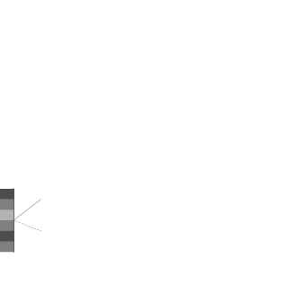
Figure 1: Schematic representation of the arrangement. The continuous and dashed lines represent the two particles

Recalling the well-known expressions $\exp(iz\cos\varphi)=\sum_{n}i^{n}J_{n}(z)\exp(in\varphi)$, with $J_{n}$ the Bessel functions, and $\cos^{2}\varphi=\frac{1}{2}+\frac{1}{2}\cos 2\varphi$, we easily obtain

$$\psi(x,X,t)=e^{iK_{0}X}\sum_{n=-\infty}^{\infty}b_{n}e^{i(2nk_{L}+k_{0})x}$$ (2)

with $b_{n}=i^{n}e^{-iw}J_{n}(-w)$ and $w=V_{0}t/2\hbar$.

The wavenumber of the particle can only be modified by double recoils. For atoms, the first one is associated with the photon absorption whereas the second one corresponds to stimulated emission. In the case of electrons, the double scattering can be understood as a stimulated Compton scattering [11].

We consider now the case of two particles. We denote by $\psi_{k_{0}K_{0}}(x,X,t)$ and $\psi_{q_{0}Q_{0}}(y,Y,t)$ two wavefunctions, with an obvious notation. When the particles are identical the usual product wavefunction $\Psi(x,X,y,Y,t)=\psi_{k_{0}K_{0}}(x,X,t)\psi_{q_{0}Q_{0}}(y,Y,t)$, valid for distinguishable particles, must be replaced by

$$\Psi(x,X,y,Y,t)=\frac{1}{\sqrt{2}}\left(\psi_{k_{0}K_{0}}(x,X,t)\psi_{q_{0}Q_{0}}(y,Y,t)\pm\psi_{k_{0}K_{0}}(y,Y,t)\psi_{q_{0}Q_{0}}(x,X,t)\right)$$ (3)

In the double sign expressions the upper one holds for bosons and the lower one for fermions.

From the above expressions one can see that, in the case of identical Particles, we have simultaneously two different interference effects. On the one hand, for both distinguishable and identical particles, the distributions $|\psi_{k_{0}K_{0}}(x,X,t)|^{2}$ display the interference effects associated with the diffraction grating. On the other hand, for identical particles we have another interference effect that is not present for distinguishable ones. This follows immediately from the term $\pm 2Re(\psi_{k_{0}K_{0}}^{*}(x,X,t)\psi_{q_{0}Q_{0}}^{*}(y,Y,t)\psi_{k_{0}K_{0}}(y,Y,t)\psi_{q_{0}Q_{0}}(x,X,t))$, contained in the expression of $|\Psi(x,X,y,Y,t)|^{2}$. This form agrees with the standard interpretation of exchange effects as interference effects [13].

3 Spatial probability distributions

In this section we evaluate the spatial distribution of simultaneous two-particle detections and the correlation functions associated with it. The simplest experimental implementation of the arrangement consists of two detectors, one fixed at a given position and the other placed at different points in successive repetitions of the experiment. In a first step we restrict our calculations to single-mode states, postponing the discussion of multi-mode ones to the next section.

The evaluation of the probability distribution is simple. We assume the detection time is fixed at $t$ and we can drop the temporal variable from all the expressions. We rewrite Eq. (2) as

$$\psi(x,X)=e^{iK_{0}X}e^{ik_{0}x}\phi(x)$$ (4)

with

$$\phi(x)=\sum_{n=-\infty}^{\infty}b_{n}e^{i2nk_{L}x}$$ (5)

With this notation the two-particle probability distribution becomes

$$|\Psi_{dis}(x,X,y,Y)|^{2}=|\phi(x)|^{2}|\phi(y)|^{2}$$ (6)

for distinguishable particles, and

$$|\Psi(x,X,y,Y)|^{2}=|\phi(x)|^{2}|\phi(y)|^{2}(1\pm\cos((K_{0}-Q_{0})(X-Y)+(k_{0}-q_{0})(x-y)))$$ (7)

for identical ones.

We assume from now on that $X=Y$, i. e., the positions of the detectors in the direction perpendicular to the light field to be equal. Several consequences easily emerge from the above expressions. In the case of identical particles, the distribution is the product of the distinguishable distribution by the term $1\pm\cos((k_{0}-q_{0})(x-y))$. The first one reflects the two-particle interferences associated with the dispersion by the light field. It is a function, through $\phi$, of $k_{L}$ and $b_{n}(V_{0}t)$ the parameters of the optical diffraction grating. That dependence is similar for both identical and distinguishable particles. On the other hand, the term containing the cosine function is related to the exchange effects. For fixed $x$ and $y$ it is only function of the initial momenta of the particles in the direction of the light field. The bunching and antibunching effects directly emerge from the above equations. In the case of bosons, for $x\approx y$ we have $|\Psi_{B}(x,X,y,X)|^{2}\approx 2|\phi(x)|^{2}|\phi(y)|^{2}$, i. e., the probability of two-boson detection almost doubles that of two distinguishable particles. For double detection at the same point, $x=y$, we have, as discussed in [9], $|\Psi_{B}(x,X,x,X)|^{2}=2|\phi(x)|^{4}$, i. e., a dependence on the fourth power of the wavefunction modulus. By contrast, for fermions we have for $x\approx y$, $|\Psi_{F}(x,X,y,X)|^{2}\approx 0$ that is the antibunching effect. When $x=y$ the probability is strictly null according to the exclusion principle. There is another situation in which the two-fermion detection probability is, for any $x$ and $y$, identically null. It occurs for equal initial momenta in the direction of the light field, $q_{0}=k_{0}$. This is so even when $K_{0}\neq Q_{0}$ (in the case of $K_{0}=Q_{0}$ it is evident that the distribution must be null because it is impossible to prepare two fermions in the same state).

Next we present a graphical representation of the above equation. As discussed before we fix one of the detectors at $y=0$ and move the other at different positions $x$. A simple calculation gives the explicit form for $\phi(x)$ and its squared modulus:

$$|\phi(x)|^{2}=1+\sum_{n,m}^{m>n}2(-1)^{n+m}J_{n}(w)J_{m}(w)\cos\left((m-n)\left(2k_{L}x+\frac{\pi}{2}\right)\right)$$ (8)

In the calculation we have used the properties $\sum_{n}|b_{n}|^{2}=1$ that derives directly from the normalization condition, and $J_{n}(-w)=(-1)^{n}J_{n}(w)$.

The normalization of $\Psi_{dis}$ is automatically guaranteed by the normalization of $\phi$. On the other hand, for identical particles $|\Psi|^{2}$ contains terms of the form $\cos((m-n)2k_{L}x+\pi/2)\cos((k_{0}-q_{0})x)$. The integration over $x$ of these terms is not null (see, for instance, [9] where similar integrations are carried out) when $(m-n)2k_{L}=\pm(k_{0}-q_{0})$. When this condition is fulfilled the normalization is not given by $|\phi(0)|^{2}\sum_{n}|b_{n}|^{2}=1$, but by the expression $|\phi(0)|^{2}(\sum_{n}|b_{n}|^{2}\pm I)=1$ with $I$ the result of the above integration.

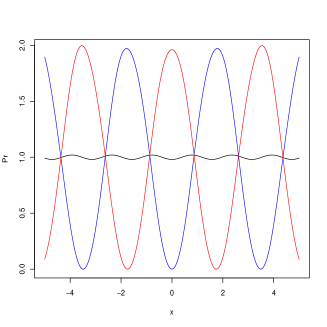
Figure 2: In the vertical axis we represent the two-particle detection probability and in the horizontal one the coordinate $x$. The red, black and blue curves correspond, respectively, to bosons, distinguishable particles and fermions. We use the values $w=0.2$, $k_{0}=0.9$, $q_{0}=-0.9$, and $k_{L}=1$.

The figure shows a large increase of the visibility of the two-particle detection probabilities for identical particles. As usual the visibility is defined as

$${\cal V}=\frac{|\Psi(x,X,0,X)|_{max}^{2}-|\Psi(x,X,0,X)|_{min}^{2}}{|\Psi(x,X,0,X)|_{max}^{2}+|\Psi(x,X,0,X)|_{min}^{2}}$$ (9)

In the case of distinguishable particles the probability approximately oscillates between $0.98$ and $1.02$, whereas for identical ones it does between $0$ and $2$. Then we have, respectively, ${\cal V}_{dis}\approx 0.02$ and ${\cal V}_{ide}\approx 1$, i. e., a very large difference.

The curves for bosons and fermions are very similar, with small changes of intensity due to the modulation introduced by the multiplicative factor $|\phi(x)|^{2}|\phi(0)|^{2}$ and a phase-$\pi$ displacement associated with the sign $\pm$ (which explains the difference between bunching and antibunching at $x\approx 0$).

Now, we briefly analyze the behavior of the correlation functions. These functions have been extensively used in the experimental study of the (anti)bunching effect of free particles released from optical lattices or magnetic traps [14, 15, 16]. In particular, in the last two references the existence of periodic correlations was shown between density fluctuations of atoms released from optical lattices. These correlations reflect the underlying structure of the lattice.

The correlation function is defined as

$$C(\eta)=\frac{1}{d}\int_{0}^{d}|\Psi(x,X,x+\eta,X)|^{2}dx$$ (10)

with $d=2\pi/k_{L}$ representing the spatial periodicity of the optical diffraction grating. In our case, this expression transforms into

$$C(\eta)=\frac{1}{d}(1\pm\cos((q_{0}-k_{0})\eta))\int_{0}^{d}|\phi(x)|^{2}|\phi(x+\eta)|^{2}dx$$ (11)

The evaluation of the integral is simple but lengthy. We only present the final result (a similar calculation can be found in [9]):

$$C(\eta)=(1\pm\cos((q_{0}-k_{0})\eta))\times$$

$$(1+2\sum_{\cal N}(-1)^{n+m+r+s}J_{n}(w)J_{m}(w)J_{r}(w)J_{s}(w)\cos(2(r-s)k_{L}\eta))$$ (12)

with ${\cal N}$ denoting the set of $n,m,r,s$ with the constrains $m>n$, $s>r$ and $m-n=\pm(r-s)$.

This correlation function is the product of two periodic functions. The first one, that in the left side, is only relevant for identical particles. For distinguishable ones it reduces to $1$ and, consequently does not vary for different initial preparations of the pairs. For identical particles it only depends on their initial momenta. For bosons it reaches maximum values for any $\eta=2N\pi/(q_{0}-k_{0})$ with $N$ an integer and minimum ones for $\eta=(2N+1)\pi/(q_{0}-k_{0})$. A similar behavior holds for fermions when an additional phase-$\pi$ is taken into account. On the other hand, the second multiplicative factor is similar for both distinguishable and identical particles and bosons and fermions. It only depends on the parameters of the optical grating, $w$ and $k_{L}$. As all the terms of the type $(r-s)k_{L}$ are contained in this factor, we have in the correlation function all the periods generated by the optical grating. As discussed in [15, 16, 9], it reflects the underlying structure of the diffraction grating.

4 Multi-mode states

Up to now, we have only considered single-mode states. Now, we move to the more realistic case of multi-mode ones. The simplest way to study them is to assume that the distribution of initial wavenumbers of each particle is a Gaussian one. The one-dimensional Gaussian distribution is given by $f(k_{0})=(4\pi)^{1/4}\sigma^{-1/2}\exp(-(k_{0}-\Lambda)^{2}/2\sigma^{2})$ with $\sigma$ the width of the distribution and $\Lambda$ its central value. The initial wavefunction reads as $\psi(x,t=0)=\int dk_{0}f(k_{0})e^{ik_{0}x}$. Note that, for the sake of simplicity, we have not included the variable $X$, which is irrelevant in the following discussion. The wavefunction after passing through the light grating is:

$$\psi(x)=\sum_{n=-\infty}^{\infty}b_{n}e^{i2nk_{L}x}\int dk_{0}f(k_{0})e^{ik_{0}x}$$

$$\sim e^{-x^{2}\sigma^{2}/2}\sum_{n=-\infty}^{\infty}b_{n}e^{i2(nk_{L}+\Lambda)x}=e^{-x^{2}\sigma^{2}/2}\psi_{\Lambda}(x)$$ (13)

where we have carried out a trivial integration over $k_{0}$, and $\psi_{\Lambda}$ represents the wavefunction of a particle with initial wavenumber $\Lambda$. For the matter of simplicity we have not included the constant coefficients of the distribution and those derived from the integration. We conclude that the multi-mode wavefunction after the interaction equals that of a single-mode particle with the central value of the distribution, but spatially modulated by a Gaussian distribution.

In the next step we consider two particles in multi-mode states, with central values $\Lambda$ and $\Upsilon$ and widths $\sigma$ and $\mu$. The probability distribution after the interaction is

$$|\Psi(x,y)|^{2}=\frac{1}{2}e^{-x^{2}\sigma^{2}}e^{-y^{2}\mu^{2}}|\phi(x)|^{2}|\phi(y)|^{2}+$$

$$\frac{1}{2}e^{-y^{2}\sigma^{2}}e^{-x^{2}\mu^{2}}|\phi(y)|^{2}|\phi(x)|^{2}\pm$$

$$e^{-(x^{2}+y^{2})(\sigma^{2}+\mu^{2})/2}|\phi(x)|^{2}|\phi(y)|^{2}\cos((x-y)(\Lambda-\Upsilon))$$ (14)

We represent this distribution. We take the same values of Fig. 2, in particular, $\Lambda=k_{0}$ and $\Upsilon=q_{0}$. For the width of the distribution we take $\sigma^{2}=\mu^{2}=0.2$.

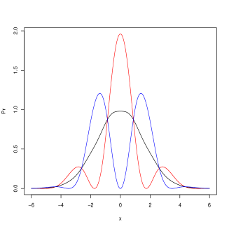
Figure 3: The same as in Fig. 2, but for multi-mode states.

As in the single-mode case, there is a notorious difference between the curves of distinguishable and identical particles. For the first one, there is an almost flat distribution in the center followed by an exponential-like decreasing superposed with small oscillations (associated with $|\phi(0)|^{2}|\phi(x)|^{2}$). On the other hand, for identical particles there is an interference pattern. In the proximities of the point $x=0$ we observe the bunching and antibunching effects. The values of the visibility are clearly different for the three figures, but not so much as in the single-mode case. These contrasts in the visibility are strongly enhanced for small values of $\sigma$.

5 Momentum space

In the two previous sections we have studied the spatial two-particle interference patterns. Now we consider the momentum space to see how the exchange effects manifest in this representation. The methodology is similar to that used above, first we consider single-mode states where the principal ideas can be analyzed in a simple way, and later we address the multi-mode case.

The wavefunction in momentum space (the momentum and wavevnumber are related by the trivial relation $p=\hbar k$, and it is justified to speak about the momentum space although really we are dealing with wavevenumbers) is given by the Fourier transform of the wavefunction in the position representation, $\Phi(k)=\int dxe^{-ikx}\psi(x)$. For the identical two-particle system we have

$$\Phi(k,q)=\int dx\int dye^{-i(kx+qy)}\Psi(x,y)=\frac{1}{\sqrt{2}}\Phi_{k_{0}}(k)\Phi_{q_{0}}(q)\pm\frac{1}{\sqrt{2}}\Phi_{k_{0}}(q)\Phi_{q_{0}}(k)$$ (15)

where the single-particle wavefunctions are characterized by the value of the initial wavenumber (for multi-mode states by the central value of the distribution).

The experimental variable to measure is the probability of detecting one particle with the value $k$ and the other with $q$. In the arrangement we must replace the detectors of the previous sections by momentum measurement devices. In a large series of measurements, for instance fixing $k$ and scanning for different values of $q$, we can compare the experimental data with the theoretical distribution:

$$|\Phi(k,q)|^{2}=\frac{1}{2}|\Phi_{k_{0}}(k)|^{2}|\Phi_{q_{0}}(q)|^{2}+\frac{1}{2}|\Phi_{k_{0}}(q)|^{2}|\Phi_{q_{0}}(k)|^{2}$$

$$\pm Re(\Phi_{k_{0}}^{*}(k)\Phi_{q_{0}}^{*}(q)\Phi_{k_{0}}(q)\Phi_{q_{0}}(k))$$ (16)

This expression shows that the probability distributions in momentum space have a structure similar to that in the position representation. In particular, for $k\approx q$ we have the bunching and antibunching effects in momentum space. This effect has been numerically discussed in [10].

To get a better understanding of that distribution we shall consider specific examples, starting with the single-mode states.

5.1 Single-mode states

We consider successively the cases of a single particle, two distinguishable Particles, and two identical ones.

One particle. This case is particularly simple because the wavefunction reduces to a superposition of Dirac’s deltas:

$$\Phi(k)=\sum_{n}b_{n}\delta(k-2nk_{L}-k_{0})$$ (17)

For a single particle the probability of finding in a momentum measurement the value $2nk_{L}+k_{0}$ is $|b_{n}|^{2}$ because, in the sense of the distributions, for $r\neq n$ the terms $\delta(k-2nk_{L}-k_{0})\delta(k-2rk_{L}-k_{0})$ are zero.

Two distinguishable particles. Now, the probability distribution is

$$|\Phi_{k_{0}}(k)|^{2}|\Phi_{q_{0}}(q)|^{2}=\sum_{n,m}|b_{n}b_{m}|^{2}\delta(k-2nk_{L}-k_{0})\delta(q-2mk_{L}-q_{0})$$ (18)

The probability of obtaining in simultaneous measurements the values $2nk_{L}+k_{0}$ and $2mk_{L}+q_{0}$, denoted as $P(n,m)$, is $|b_{n}b_{m}|^{2}$.

To illustrate the form of this probability we graphically Represent it in Fig. 4 it for the lower values of $n$ and $m$. Note that this probability is equal to the probability of $n$ absorptions by the particle with initial wavenumber $k_{0}$ and $m$ by that with $q_{0}$. For small values of $w$ there is only one absorption. When $w$ increases the probability of two absorptions becomes dominant. The probability of symmetric absorption (one photon each particle, $P(1,1)$) is much larger than the asymmetric one (one particle two photons and the other none, $P(0,2)$). For larger values of $w$ the terms with three absorptions become important. However, here, there is again a notorious difference between $P(1,2)$ that increases with $w$ and $P(0,3)$ that remains negligible for all the range of values considered. At the end of the graphic, the term $P(2,2)$ becomes comparable to (or larger than) the other terms.

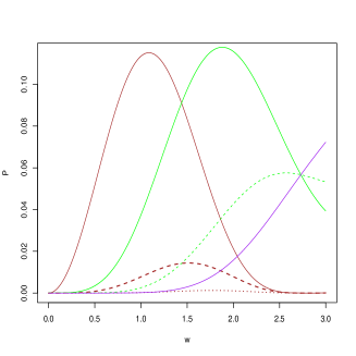
Figure 4: Representation of the probability P(n,m) versus w. The brown curves correspond to $P(0,1)$ (continuous), $P(0,2)$ (dashed), and $P(0,3)$ (dotted), the green ones to $P(1,1)$ (continuous), and $P(1,2)$ (dashed), and the purple one to $P(2,2)$.

Two identical particles. The two direct terms in $|\Phi(k,q)|^{2}$ are similar to those for distinguishable particles. We evaluate now the term associated with the exchange effects:

$$\Phi_{k_{0}}^{*}(k)\Phi_{q_{0}}^{*}(q)\Phi_{k_{0}}(q)\Phi_{q_{0}}(k)=$$

$$\sum_{n,m,r,s}b_{n}^{*}b_{m}^{*}b_{r}b_{s}\delta(k-2nk_{L}-k_{0})\times$$

$$\delta(q-2mk_{L}-q_{0})\delta(q-2rk_{L}-k_{0})\delta(k-2sk_{L}-q_{0})$$ (19)

The product of the two deltas containing $k$ is zero (in the sense of the distributions) unless the relation $2nk_{L}+k_{0}=2sk_{L}+q_{0}$ holds. Similarly, we must have $2mk_{L}+q_{0}=2rk_{L}+k_{0}$ in order for the product of the deltas containing $q$ not be null. These two relations can be expressed as

$$n-s=N\;;\;m-r=-N\;;\;N=\frac{q_{0}-k_{0}}{2k_{L}}$$ (20)

with $N$ an integer. The difference between the initial wavenumbers must be an integer number of times $2k_{L}$.

When these relations hold, we have that the terms related to the deltas containing $n$ and $m$ must be rewritten as

$$\frac{1}{2}|b_{n}b_{m}|^{2}\delta(k-2nk_{L}-k_{0})\delta(q-2mk_{L}-q_{0})+$$

$$\frac{1}{2}|b_{n}b_{m}|^{2}\delta(q-2nk_{L}-k_{0})\delta(k-2mk_{L}-q_{0})\pm$$

$$Re(b_{n}^{*}b_{m}^{*}b_{m+N}b_{n-N})\delta(k-2nk_{L}-k_{0})\delta(q-2mk_{L}-q_{0})$$ (21)

The two first terms correspond to the absorption of $n$ photons by a particle with initial wavenumber $k_{0}$ and $m$ by one with $q_{0}$. If $(q_{0}-k_{0})/2k_{L}$ is not an integer, the third term does not contribute and we have the two final wavenumbers $2nk_{L}+k_{0}$ and $2mk_{L}+q_{0}$ with probability $|b_{n}b_{m}|^{2}$. On the other hand, when the condition holds we obtain the same final wavevenumbers $2nk_{L}+k_{0}$ and $2mk_{L}+q_{0}$, but with probability

$$P_{N}(n,m)=|b_{n}b_{m}|^{2}\pm Re(b_{n}^{*}b_{m}^{*}b_{m+N}b_{n-N})$$ (22)

This result can easily be understood in terms of indistinguishability of alternatives. If the final wavenumbers are the same for both types of absorptions, we cannot distinguish if the final result corresponds to the alternative of absorptions $n$ and $m$, or to the other alternative, $n-N$ and $m+N$. In quantum theory the amplitudes of probability for indistinguishable alternatives must be added, obtaining an interference effect. The indistinguishable alternatives correspond to different numbers of absorptions yielding the same final wavenumbers. The situation is different for distinguishable particles. In this case, we can know in principle at any instant if the particle is of one type (that whose wavenumber is denoted by $k$) or the other (wavenumber $q$) and, consequently, if its initial wavenumber was $k_{0}$ or $q_{0}$. Then one particle of the first kind cannot reach the final wavenumber $2nk_{L}+k_{0}$ by $n-N$ absorptions. There are not different alternatives to reach the final wavenumber and, there is not an interference effect.

Figure 5: Representation of the exchange effects. Black and white circles represent particles labeled by $k$ and $q$. (a) The standard (anti)bunching effect in the spatial representation. The detections can occur in two alternative ways, these represented by the continuous and dashed lines. (b) The same effect in momentum space. The dashed horizontal lines correspond to the two momenta at which the particles are detected and the continuous vertical ones to the trajectories in momentum space. The (anti)bunching is observed when the two final momenta are very close. (c) The effect discussed in this paper. The dotted lines correspond to the initial momenta. The arrows represent the absorption of photons. Being the particles identical the two represented alternatives are indistinguishable.

We remark that this novel exchange effect is different from (anti)bunching (see Fig. 5). The last one only takes place when we consider particles very close in momentum space. In contrast, the effect described here only depends on the initial values of the momenta (which can be rather different for all the cases with $N\neq 0$) and can occur for well-separated final momenta.

The previously described effect is a purely quantum one. To justify this statement we show that it cannot be described by a classical treatment. We use a qualitative model where the particles collide with the photons and the collisions are ruled by the classical law of momentum conservation (classical description of the Compton effect assuming the existence of photons). We assume that all of the momentum of the photon is transferred to the particle, in such a way that its momentum changes from $p_{0}$ to $p_{0}+\hbar k_{L}$. In the cases with $2n$ collisions the final momentum of the particle would be the same predicted by quantum theory. However, in the absence of additional unnatural assumptions, the classical theory allows for odd numbers of collisions. The agreement between the model and quantum theory would be even worse for couples of particles. Classically, both particles behave in an independent way, and the stochastic collision events are uncorrelated. The probability of one particle experiencing $2n$ collisions and the other $2m$ factorizes. The result would be similar to that for quantum distinguishable particles. In conclusion, in the classical model (a reasonable one) there is not room for the previous exchange effect.

Next we represent these probabilities for a particular example. A simple calculation using the expression for $b_{n}$ and the property of the Bessel functions $J_{-n}(w)=(-1)^{n}J_{n}(w)$ gives $P_{0}(1,0)=J_{1}^{2}J_{0}^{2}\pm J_{1}^{2}J_{0}^{2}$, $P_{1}(1,0)=J_{1}^{2}J_{0}^{2}\pm J_{1}^{2}J_{0}^{2}$ and $P_{-1}(1,0)=J_{1}^{2}J_{0}^{2}\mp J_{1}^{2}J_{0}J_{2}$. We see that $P_{0}(1,0)=P_{1}(1,0)$.

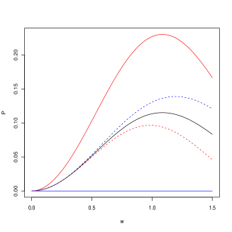
Figure 6: Representation of the probability P of finding the final wavenumbers $2nk_{L}+k_{0}$ and $2mk_{L}+q_{0}$ versus w. The black curve represents the distinguishable case for $n=1$ and $m=0$. The red and blue ones correspond to bosons and fermions with $N=1$ (continuous) and $N=-1$ (dashed).

The figure clearly shows that the probabilities of finding the particle in the targeted final wavenumber state are different for the all the cases. For $N=1$ the detection rate notoriously increases for bosons, whereas it becomes null for fermions. The detection rate is not always enhanced for bosons; for $N=-1$ it is smaller than that of distinguishable particles. Similarly, the fermion rate can increase with respect to that of distinguishable particles (also $N=-1$).

5.2 Multi-mode states

In this subsection we analyze how the above results are modified in the more realistic case of multi-mode distributions. We mainly restrict our considerations, as in Sect. 4, to Gaussian distributions which can be tackled analytically. As in the previous subsection we consider successively the cases of a single particle, two distinguishable particles, and two identical ones.

One particle. The wavefunction in momentum space for a particle with a multi-mode distribution $f(k_{0})$ of initial wavenumbers is easily obtained:

$$\Phi(k)=\int dxe^{-ikx}\psi(x)=\int dxe^{-ikx}\sum_{n}\int dk_{0}f(k_{0})b_{n}e^{i(2nk_{L}+k_{0})x}=$$

$$\sum_{n}\int dk_{0}f(k_{0})b_{n}\delta(k-2nk_{L}-k_{0})=\sum_{n}b_{n}f(k-2nk_{L})$$ (23)

The probability of finding the particle with final wavenumber $k$ is $|\Phi(k)|^{2}=\sum_{n,m}b_{n}^{*}b_{m}f^{*}(k-2nk_{L})f(k-2mk_{L})$. If the mode distribution is a Dirac’s delta (the single-mode distribution), $f(k_{0})=\delta(k_{0}-K_{0})$, the probability becomes $|\Phi(k)|^{2}=\sum_{n}|b_{n}|^{2}\delta(k-2nk_{L}-K_{0})$.

When the initial distribution is a Gaussian, $f(k_{0})\sim e^{-(k_{0}-\Lambda)^{2}/2\sigma^{2}}$, we have

$$|\Phi(k)|^{2}\sim\sum_{n,m}b_{n}^{*}b_{m}e^{-(k-2nk_{L}-\Lambda)^{2}/2\sigma^{2}}e^{-(k-2mk_{L}-\Lambda)^{2}/2\sigma^{2}}$$ (24)

These two exponentials correspond to two Gaussians with the same width of the initial ones, but centered around $2nk_{L}+\Lambda$ and $2mk_{L}+\Lambda$. Two different regimes can be obtained. For $2k_{L}\gg\sigma$ we have that the overlapping between the Gaussians centered around $2nk_{L}+\Lambda$ and $2(n\pm 1)k_{L}+\Lambda$ (and, of course, any $m$ with $|n\pm m|>1$) is negligible. The sum in the above expression reduces to the diagonal terms, $|\Phi(k)|^{2}\simeq\sum_{n}|b_{n}|^{2}e^{-(k-2nk_{L}-\Lambda)^{2}/\sigma^{2}}$. After the interaction, we can only detect the particle with wavenumbers contained in the Gaussian distributions centered in the points $2nk_{L}+\Lambda$ (with $1/\sqrt{2}$ times the width of the initial one). There is not a contribution of the crossed terms to the probability of detection. In the limit of very peaked Gaussians we recover the behavior described by Dirac’s delta distributions. The other regime takes place when $\sigma\geq 2k_{L}$. In this case, there is a non-negligible overlapping between the distributions centered around $2nk_{L}+\Lambda$ and $2(n\pm 1)k_{L}+\Lambda$ (and, perhaps, the other $m$ with $|n-m|>1$). The crossed terms can no longer be neglected, leading to interference terms. These interference terms can be understood by the impossibility of distinguishing if a particle detected with wavenumber $k$ belongs to one or the other of the distributions.

Two distinguishable particles. The discussion closely follows that of one particle. If the initial distributions of the particles are $f(k_{0})$ and $g(k_{0})$ the probability of finding one particle with $k$ and the other with $q$ is

$$|\Phi_{f}(k)|^{2}|\Phi_{g}(q)|^{2}\sim\sum_{n,m,r,s}b_{n}^{*}b_{m}b_{r}^{*}b_{s}f^{*}(k-2nk_{L})f(k-2mk_{L})g^{*}(q-2rk_{L})g(q-2sk_{L})$$ (25)

We assume the two distributions to be Gaussian ones. For $2k_{L}\gg\sigma$ and $2k_{L}\gg\mu$ we have that the overlappings between the Gaussians centered around $2nk_{L}+\Lambda$ and $2(n\pm 1)k_{L}+\Lambda$ and $2nk_{L}+\Upsilon$ and $2(n\pm 1)k_{L}+\Upsilon$ are negligible, becoming the probability $|\Phi_{f}(k)|^{2}|\Phi_{g}(q)|^{2}\simeq\sum_{n,m}|b_{n}b_{m}|^{2}e^{-(k-2nk_{L}-\Lambda)^{2}/\sigma^{2}}e^{-(q-2nk_{L}-\Upsilon)^{2}/\mu^{2}}$. The probability is the product of the one-particle distributions without crossed terms. When the conditions $\sigma\geq 2k_{L}$ and/or $\mu\geq 2k_{L}$ hold we have crossed terms leading to interference effects.

Two identical particles. The two-particle probability contains the terms of the form $|\Phi_{f}(k)|^{2}|\Phi_{g}(q)|^{2}$, which can be treated as before, and the exchange term that transforms into $\sum_{n,m,r,s}Re(b_{n}^{*}f^{*}(k-2nk_{L})b_{m}^{*}g^{*}(q-2mk_{L})b_{r}f(q-2rk_{L})b_{s}g(k-2sk_{L}))$. We again consider Gaussian distributions, for which the exchange term reads proportional to

$$\sum_{n,m,r,s}Re(b_{n}^{*}b_{m}^{*}b_{r}b_{s})e^{-(k-2nk_{L}-\Lambda)^{2}/2\sigma^{2}}\times$$

$$e^{-(q-2mk_{L}-\Upsilon)^{2}/2\mu^{2}}e^{-(q-2rk_{L}-\Lambda)^{2}/2\sigma^{2}}e^{-(k-2sk_{L}-\Upsilon)^{2}/2\mu^{2}}$$ (26)

For the sake of simplicity we take $\sigma=\mu$. For $|2(n-s)k_{L}+\Lambda-\Upsilon)|\gg\sigma$ or $|2(m-r)k_{L}-\Lambda+\Upsilon)|\gg\sigma$ (for any $n$ and $s$ and $m$ and $r$) the overlapping between the curves is negligible and the product of the two distributions with the same argument ($k$ or $q$) is almost null. The contribution of the exchange terms can be neglected. In contrast, when $|2(n-s)k_{L}+\Lambda-\Upsilon)|\leq\sigma$ for some $n$ and $s$ and $|2(m-r)k_{L}-\Lambda+\Upsilon)|\leq\sigma$ for some $m$ and $r$ the product of the distributions cannot be neglected. The exchange effects become important in this case. However, the conditions for the presence of the exchange effect are much less stringent than in the case of single-mode states.

6 Discussion

We have analyzed in this work the extension of the Kapitza-Dirac effect to the case of two-particle systems. The spatial two-particle detection patterns display notorious differences for distinguishable particles and fermions and bosons, in particular for the shape and visibility of the interference figure.

We have also shown the existence of a novel exchange effect in momentum space. The effect, which modifies the distribution of particles detected with given momenta, only occurs for some values of the initial momenta of the particles (or in the case of multi-mode states for some values of the parameters of the initial momenta distributions). For multi-mode states these conditions are much less stringent than for single-mode ones. The verification of this effect would be interesting in several aspects. Exchanges effects are a striking manifestation of the departure between classical and quantum descriptions of physical systems. Any new example of these differences is worth investigating. The novel effect has no relation with other exchange effects such as (anti)bunching, exclusion in atoms, or degeneracy in gases. The physical underlying mechanisms are different, in our case, different numbers of photon absorptions. Moreover, the confirmation of the effect would corroborate the validity of the (anti)symmetrization principle in a framework where strong interactions with other types of particles are present.

In this paper, we have only considered the spatial part of the wavefunction. This is equivalent to assume that the spin states (and the electronic states for atoms) are symmetric and do not play any role in the problem. The extension to the case of antisymmetric spin or electronic states, where the relative sign of the spatial part of the wavefunction can be reversed, is simple.

Some other aspects of our approach must be commented on. The wavefunctions have just been evaluated after the interaction with the optical grating. The detectors must be placed at these positions, and consequently, we are in the near-field regime. However, in this type of problems one usually works in the far-field one [7]. In the free evolution of the particles between both regimes there is a dispersion of the wavefunctions. Fortunately, that evolution is simple (free evolution) and can easily be described. For instance, in the spatial picture we have that the width of the Gaussian packet increases with time. As the momentum peaks are determined via spatial detection [7] we must take into account that broadening to correctly interpret the data. For well-separated peaks the effects of the spreading are negligible. For peaks with appreciable overlapping the range of values of the initial momenta for which the exchange effect described in this paper takes place increases (as we can easily see with an argument similar to that used for multi-mode states in subsection 5.2). An exact treatment of the problem would require a quantitative evaluation of the evolution of the multi-mode states, instead of the qualitative one presented here. However, this will be presented elsewhere. Another important aspect of the problem is the question of the coherence between the two particles. As is well-known, when they are only partially coherent the two-particle interference properties, in particular the visibility, are modified. Thus, the relative coherence of the two particles should be checked for every type of source of pairs of particles. When it is only partial we should introduce the necessary modifications in the formalism. In our proposal, there is an additional question similar to that of the partial coherence: we must analyze if the overlapping between the wavefunctions is complete or partial (see also the next paragraph). In the first case we can use a completely (anti)symmetrized wavefunction. In the second one, we should include in the wavefunction (or in a density matrix) the property of partial overlapping. This is a subject worth analyzing since, as far as we know, it is not considered in the literature. Here, by a matter of simplicity, we have assumed complete coherence between both particles in the two senses, coherence and overlapping.

The last question we briefly address here is the possibility of experimentally testing the above effects. In the space representation, the interchange effects are present when there is a non-negligible overlapping between the wavefunctions of the two particles. Then we must prepare the particles in such a way that they have a non-negligible overlapping at the time they reach the optical grating. Several sources of identical particles, such as Bose-Einstein condensates, optical lattices, or magnetic traps have recently been used to study correlation functions [14, 15, 16]. If we would be able to select the cases in which only two particles are released from any of the above devices we would have an efficient source for our problem. We would also carefully test that the times of the arrival of the two particles to the optical grating are close enough. In terms of wavepacket spread, the peaks of the two probability distributions must reach the optical grating at the same time. On the other hand, the interaction strength is given, as in the one-particle case, by the parameter $w$. Using the same values of the single particle arrangement [11] we can reach an appreciable value for the number of pairs diffracted.

Acknowledgments We acknowledge partial support from MEC (CGL 2007-60797).

References

- [1] P. L. Kapitza and P. A. M. Dirac, Proc. Cambridge Philos. Soc. 29, 297 (1933).
- [2] C. S. Adams, M. Sigel, and J. Mlynek, Phys. Rep. 240, 143 (1994).
- [3] P. L. Gould, G. A. Ruff, and D. E. Pritchard, Phys. Rev. Lett. 56, 827 (1986).
- [4] P. J. Martin, B. G. Oldaker, A. H. Miklich, and D. E. Pritchard, Phys. Rev. Lett. 60, 515 (1988).
- [5] S. B. Cahn, A. Kumarakrishnan, U. Shim, T. Sleator, P. R. Berman, and B. Dubetsky, Phys. Rev. Lett. 79 784 (1997).
- [6] D. L. Freimund, K. Aflatooni, and H. Batelaan, Nature 413, 142 (2001).
- [7] D. L. Freimund and H. Batelaan, Phys. Rev. Lett. 89 283602 (2002).
- [8] C. K. Hong, Z. Y. Ou, and L. Mandel, Phys. Rev. Lett. 59, 2044 (1987).
- [9] P. Sancho, J. Phys. B 43 065504 (2010).
- [10] G. Lenz, P. Pax, and P. Meystre, Phys. Rev. A 48, 1707 (1993).
- [11] H. Batelaan, Contemp. Phys. 41, 369 (2000).
- [12] M. V. Fedorov, JETP 52, 1434 (1967).
- [13] U. Fano, Am. J. Phys. 29, 539 (1961).
- [14] T. Jeltes, et al., Nature 445, 402 (2007).
- [15] S. Föllling, F. Gerbier, A. Widera, O. Mandel, T. Gericke, and I. Bloch, Nature 434, 481 (2005).
- [16] T. Rom, Th. Best, D. Van Oosten, U. Schneider, S. Föllling, B. Paredes, and I. Bloch, Nature 444, 733 (2006).