Connectivity Graphs of Uncertainty Regions

Abstract

We study connectivity relations among points, where the precise location of each input point lies in a region of uncertainty. We distinguish two fundamental scenarios under which uncertainty arises. In the favorable Best-Case Uncertainty (BU), each input point can be chosen from a given set to yield the best possible objective value. In the unfavorable Worst-Case Uncertainty (WU), the input set has worst possible objective value among all possible point locations, which are uncertain due, for example, to imprecise data.

We consider these notions of uncertainty for the bottleneck spanning tree problem, giving rise to the following Best-Case Connectivity with Uncertainty (BCU) problem: Given a family of geometric regions, choose one point per region, such that the longest edge length of an associated geometric spanning tree is minimized. We show that this problem is NP-hard even for very simple scenarios in which the regions are line segments or squares. On the other hand, we give an exact solution for the case in which there are $n+k$ regions, where $k$ of the regions are line segments and $n$ of the regions are fixed points. We then give approximation algorithms for cases where the regions are either all line segments or all unit discs. We also provide approximation methods for the corresponding Worst-Case Connectivity with Uncertainty (WCU) problem: Given a set of uncertainty regions, find the minimal distance $r$ such that for any choice of points, one per region, there is a spanning tree among the points with edge length at most $r$.

1 Introduction

Finding an optimally connected substructure in a network is one of the fundamental combinatorial optimization problems in network design. The standard problem of minimizing the total edge cost in the network amounts to finding a minimum spanning tree, which can be computed by straightforward greedy methods. A closely related problem that has gained in importance in the context of wireless networking is to consider the “bottleneck” problem of minimizing the length of the longest edge. A solution to this problem allows one to choose a point set of lowest power, where equi-power routers are to be placed at nodes, such that a message can be relayed between any two nodes. However, the situation changes when the locations of devices becomes part of the problem: How should each location be chosen from a given neighborhood, such that the solution to the resulting bottleneck connectivity problem is minimized? The neighborhoods can be the result of imprecise input data, or simply arise from a geometric range of possible locations; depending on the scenario, the choice of locations can be optimistic (i.e., best case) or adversarial (i.e., worst case).

Let $U$, $|U|=n$, denote a family of uncertainty regions, e.g., a family of disks, squares, line segments or pairs of points. For each uncertainty region $u_{i}\in U$, $1\leq i\leq n$, one point $p_{i}$ is to be chosen inside this region $u_{i}$. Let $P$ be the set of points chosen. For a value $\alpha\in\mathbb{R}$, we define the connectivity graph $G_{\alpha}=(V,E)$ of $P$ with respect to $\alpha$ as follows: $V=P$ and $E=\{(p_{i},p_{j})\in P\times P,\|p_{i}-p_{j}\|_{2}\leq 2\alpha\}$. Thus, the graph connects a pair of points with an edge whenever closed disks of radius $\alpha$ centered at these points intersect. We can now formally define the main problem, Best-Case Connectivity with Uncertainty (BCU), that we study in this paper.

The BCU Problem. Given a set $U=\{u_{1},\ldots,u_{n}\}$ of $n$ uncertainty regions, find the minimum value $\alpha$ for which there exists a choice of point set $P=\{p_{1},\ldots,p_{n}\},p_{i}\in u_{i}$, such that the connectivity graph $G_{\alpha}$ of $P$ is connected.

We further study a closely related problem, Worst-Case Connectivity with Uncertainty (WCU):

The WCU Problem. Given a set $U=\{u_{1},\ldots,u_{n}\}$ of $n$ uncertainty regions, find the minimum value $\alpha$, such that for any choice of point set $P=\{p_{1},\ldots,p_{n}\},p_{i}\in u_{i},$ the connectivity graph $G_{\alpha}$ of $P$ is connected.

1.1 Related Work.

If the $n$ uncertainty regions are points (in other words, there is no uncertainty), then finding the minimum $\alpha$ for which the connectivity graph is connected amounts to finding a minimum Euclidean Bottleneck Spanning Tree (MBST) on the points. Because minimum spanning trees (MSTs) are also MBSTs, a solution can be found in time $O(n\log{n})$.

Closely related to our BCU and WCU problems is the well-studied family of range assignment problems. In these problems, the disks centered at the points can be of different radius, and the goal is to minimize the total power consumption under the constraint that the network satisfies certain structural properties like connectivity, strong connectivity, or a particular broadcast property. Most of the work on these problems has considered point sets rather than uncertainty regions (see cps-opapr-00 ; lp-eaasb-02 ; lp-ptasb-05 ; SCG06 ; fuchs-06 ). Thus our work provides an early exploration of connectivity problems, arising in the context of wireless networks, for points lying in nontrivial uncertainty regions.

The minimum spanning tree problem (MST) has been studied in the setting of uncertainty regions. Yang et al. Yang07 showed that the problem of computing a spanning tree that minimizes the total edge length is NP-hard if the uncertainty regions are non-overlapping unit disks or rectangles. They also give a polynomial-time approximation scheme (PTAS) for the case in which the uncertainty regions are unit disks; this is notably different from our problem, which does not admit a PTAS, unless P=NP. Further approximation results for minimization and maximization versions of the MST with uncertainty were provided by Dorrigiv et al. dfh+-mmwst-12 . Another optimization problem with neighborhoods that have received attention is the Traveling Salesman Problem; e.g. see ah-aagcp-94 ; mm-aagtn-95 ; gl-faatn-99 ; dm-aatnp-01 ; delm-tsp-03 ; bgk+-tnvs-05 ; m-ptnfr-07 . The bottleneck version of TSP is known to be NP-hard (Garey_Johnson79, , p. 212). A $2$-approximation has been known since 1984 parker_rardin84 .

Other work on geometric optimization with uncertainty regions has been framed using the notions of imprecise data or neighborhoods. For studies of shortest paths with uncertainty regions see pk-aspas-10 ; dmmw-rsprm-14 ; dmm-mspip-15 . For a more general treatment and discussion of problems such as convex hulls, see Löffler and van Kreveld lv-lschi-10 , who also considered the size of bounding boxs, diameters and related problems in lv-lbbsm-10 . A discrete variant in $d$-dimensional space was considered by Ding and Xu dx-scccp-11 , who studied the problem of picking one representative each from a family of finite sets, such that the resulting set has a small enclosing hypersphere. Fiala et al. fiala05 considered “systems of distant representatives”, which amounts to maximizing the minimum distance between selected points. This is related to but different from our work in this paper: we aim for minimizing the maximum length in a spanning tree.

Another angle is to consider topological changes under uncertainty: when does the structure of an optimal solution change when the input data is perturbed? Abellanas et al. ahr-stdt-99 studied this structure with respect to the largest perturbation of a set of planar points that keeps the Delaunay triangulation unchanged. Conversely, problems of determining a necessary perturbation in order to achieve a desired change have also been studied; e.g., see Arkin et al.adk+-ct-11 for deciding whether a given set of neighborhoods has a convex stabber, which amounts to deciding whether a given set can be moved into a convex position. For further discussions of related problems, see the excellent exposition by Löffler and van Kreveld lv-lschi-10 .

1.2 Our Main Results.

After showing that several variants of BCU are NP-hard (some even to approximate), we give exact and approximation algorithms for certain variants. Given the geometric nature of our problems, we use the Euclidean measure of distance. Our main results are as follows:

1. We show that BCU is NP-hard even in the simple cases in which the uncertainty regions are point pairs and vertical line segments, respectively. Our proof technique also works when the regions are all squares. We further show that it is NP-hard to approximate BCU within a factor less than $\sqrt{5}/2$ when the uncertainty regions are pairs of points. See Section 2.

2. We present an exact algorithm for BCU when the instance consists of $n$ fixed points and $k$ line segments. The algorithm is polynomial in $n$ for constant $k$. The output of this algorithm is correct up to precision $\delta$, $\delta>0$. See Section 3.

3. For uncertainty regions that are all unit disks, we give a simple constant additive approximation algorithm for BCU. A slight modification of this algorithm gives a constant multiplicative approximation in case the disks are non-overlapping. See Section 4.

4. We provide approximation results for the WCU. In particular, we establish methods with additive and multiplicative performance guarantees. See Section 5.

2 Hardness Results for BCU

We prove hardness results for three variants of the BCU problem. Our first main result shows NP-hardness when the uncertainty regions are point pairs (Theorem 2.1). Interestingly, this result also implies a hardness of approximation result for the case of point pairs (Theorem 2.2), and NP-hardness when the uncertainty regions are line segments (Theorem 2.3). Our second main result shows NP-hardness when the uncertainty regions are unit squares (Theorem 2.4). We assume, in all cases, that the uncertainty regions are non-overlapping. All of our reductions are from Planar 3-SAT – in other words 3-SAT with the added condition that the input formula can be represented as a planar graph.

2.1 BCU when uncertainty regions are point pairs.

We consider the BCU problem for uncertainty regions of vertically aligned pairs of points, unit distance apart with integer coordinates. We study the decision version of the BCU problem for $\alpha=1$, i.e., we want to decide if $G_{\alpha}=G_{1}$ is connected for some choice of points, one for each uncertainty pair.

Theorem 2.1

It is NP-hard to find an exact solution to the BCU problem for the case in which the regions of uncertainty are point pairs that have a vertical distance of length one.

Proof

We show this problem is NP-hard, using a reduction from the following formulation of Planar 3-SAT. Let $\Phi=(X,C)$ be an instance of 3-SAT, with variables $X=\{x_{1},\ldots,x_{n}\}$ and clauses $C=\{c_{1},\ldots,c_{m}\}$. Each clause consists of exactly three literals, each a variable or its negation. For such an instance, we define a formula graph $H(\Phi)$ as follows: $H(\Phi)=(V,E)$ with vertex set $V=X\cup C$ and edge set $E=E_{1}\cup E_{2}$, such that $E_{1}=\{(x_{i},x_{i+1})|i<n\}$, and $E_{2}=\{(x_{i},c_{j})|c_{j}\mbox{ contains }x_{i}\mbox{ or }\overline{x_{i}}\}$. A Planar 3-SAT instance is one whose corresponding formula graph $H(\Phi)$ is planar. In the Planar 3-SAT problem, our goal is to determine whether a given Planar 3-SAT instance $\Phi$ is satisfiable. This problem is known to be NP-complete Garey_Johnson79 ; Lichtenstein .

Our reduction makes use of the fact that, given a Planar 3-SAT instance $\Phi$ with formula graph $H(\Phi)$, this graph has a planar layout on an $O(n+m)\times O(n+m)$ grid Duchet ; Rosenstiehl . Further, in this layout, the vertices (variables and clauses) can be drawn as horizontal line segments and edges as vertical line segments. Henceforth, we equate the formula graph $H(\Phi)$ with the planar layout we have described above.

To reduce from Planar 3-SAT to BCU when the uncertainty regions are pairs of points, we design various gadgets. Specifically, given a layout of a Planar 3-SAT instance using line segments as described above, we replace each horizontal line segment corresponding to a variable by a variable gadget, each horizontal line segment corresponding to a clause by a clause gadget, and each vertical line segment corresponding to an edge in $E_{1}$ by a variable-variable connector and each one corresponding to an edge in $E_{2}$ by a variable-clause connector. Below we will argue that there exists a choice of point in each of these uncertainty pairs such that the connectivity graph for $\alpha=1$, $G_{1}$, is connected if and only if the corresponding Planar 3-SAT instance is satisfiable.

Overview of the gadgets

We present the main ideas behind the clause gadgets, variable gadgets, and connector gadgets mentioned above.

A clause gadget is designed so that it contains three “gates”, one for each of the literals in the clause. The gate for each literal is either on the top or the bottom of the clause gadget, depending on whether the literal appears above or below the clause in the planar grid layout of $H(\Phi)$. For the connectivity subgraph corresponding to the clause to be connected to the rest of the graph in $G_{1}$, at least one of these three gates must be open. This corresponds to setting the literal to True in the clause. This, in turn, ensures that the clause is satisfied.

The role of a variable gadget is to choose and propagate a truth value for the variable to all the clauses containing it in a consistent manner. The variable gadget contains three types of constructs. Type $I$ and type $II$ constructs help link the variable to all the clauses that contain it and are either above or below it. We have one such type $I$-type $II$ pair for every occurrence of the variable in a clause. A construct of type $III$ is used to ensure that the subgraph corresponding to the variable gadget can be connected if and only if the truth assignment to the variable in all the copies of type $I$-type $II$ pairs are the same. Our construction also prevents subgraphs arising from parts of a variable gadget from being connected through other parts of $G_{1}$.

The variable and clause gadgets are linked to each other using two types of connectors. A clause-variable connector replaces an edge of $H(\Phi)$ between a clause vertex and a variable vertex in such a way that points chosen in the corresponding gadgets can be connected through it if and only if the truth value of the variable is consistent with its occurrence (as a literal) in the clause. A variable-variable connector replaces an edge of $H(\Phi)$ between two variable vertices. Points in one variable gadget can be connected to those in another variable gadget via points chosen in the variable-variable connector irrespective of the choice of truth values for each variable gadget.

Having given the overview of the reduction, we now provide a detailed proof by first describing the different gadgets in detail and then arguing the correctness of our reduction.

The clause gadget

Figure 1 depicts a schema that describes the functioning of a clause gadget. Each gate in the schema represents the entry of a connection to a literal, with an open gate representing a contribution of True. If all gates are closed, then, as suggested by the schema, it is possible that the connectivity graph of the clause gadget is connected, but it is isolated from the rest of the graph. Also, as the schema suggests, if gates to two literals $x_{i}$ and $x_{j}$ are both open, then connections are created between the clause gadget and the gadgets for the literals, but no connection via the clause gadget is made between the variable gadgets.

Figure 1: Schema of the clause gadget. When a gray gate is open the entire clause gadget can be connected to the rest of the graph.

The shape of the clause gadget can be adapted to meet the requirements of the clause vertex it represents in the planar layout of $H(\Phi)$ (e.g., the length of the horizontal line segment representing a particular clause gadget in the planar layout of $H(\Phi)$ by line segments; however many of the horizontal segments representing literals contained in the clause lie below the segment representing the clause and however many above). Figure 2 shows an example of a clause gadget where, in the representation of $H(\Phi)$, the clause was represented by a horizontal segment connected to one horizontal variable segment lying above, and two horizontal variable segments lying below the segment for the clause. The clause gadget is flexible, as its size can be adjusted by adding more uncertainty pairs to the sequence between two connections to the variable gadgets, and to the sequence between connections to variable gadgets and the left and right sides of the gadget. Furthermore, in a straightforward manner we can modify the clause gadget to move the connection to a particular variable gadget vertically by one unit without moving the entire clause gadget; e.g., the uncertainty pairs in the gray box in Figure 2 can be moved up by one unit.

Consider the three uncertainty pairs with white and gray points in Figure 2. If all three of the white points are chosen, then it is easy to see that, while points can be chosen so that the connectivity subgraph arising from pairs in the clause gadget can be made connected, no such subgraph can be connected to the rest of $G_{1}$ for any choice of points in the remaining uncertainty pairs. If a gray point is chosen from a white-gray pair, then the dashed edges shown incident to the pair do not belong to $G_{1}$.

Figure 2: An example clause gadget. As shown, aside from vertical sequences of uncertainty pairs leading to variable gadgets, there are no other uncertainty pairs in the vicinity of the clause gadget. The graph $G_{1}$ can be connected only if at least one of the gray points is chosen; that is, the attached literal is set to True. The gate inside the gray box can be moved up one unit to meet variable-clause connectors at different heights, if necessary.

Each of the three white-gray uncertainty pairs is connected to a variable gadget by a sequence of vertical uncertainty pairs. The choice of a gray point, shown in the schema as an open gate, is intended to mean that the literal (a variable or its negation) connecting to this open gate contributes a True to the clause. Note that the clause gadget never connects two variable gadgets.

Next, we outline how variable gadgets transmit truth values and how consistency of truth assignments is assured.

The variable gadget

An example of the variable gadget is shown in Figure 3. Let the uncertainty pair at the extreme left of the variable gadget be the reference pair for this variable. We adopt the interpretation that the choice of black point in the reference pair means a setting of True to the variable and the choice of gray point means a setting of False to the variable.

Figure 3: An example variable gadget.

In order for the constructs of type $I$, $II$, and $III$ to function as described above, in the Overview of the gadgets, we require that the following two properties hold: (1) for all variable gadgets, $G_{1}$ is connected only if the subgraph of $G_{1}$ restricted to points chosen in a given variable gadget is connected; and, (2) the subgraph of $G_{1}$ restricted to points chosen in a variable gadget can be connected if and only if the truth values in type $I$ and $II$ constructs are consistent with the reference pair (as these are the parts of the gadget that propagate truth values to clause gadgets). Together, these properties ensure that for $G_{1}$ to be connected, the points chosen from variable gadgets must be internally connected and, in turn, each variable gadget must propagate consistent truth values to the clause gadgets that are connected to it via connector gadgets. We prove these two properties now.

Recall that the clause gadget connects to the literals that are satisfied (only) by opening gates, and that no two open gates are connected through the clause gadget. As such, there cannot be a path in $G_{1}$ joining points in two (possibly indistinct) variable gadgets through points in a clause gadget. In addition, the edges $E_{1}$ join the variable vertices (horizontal lines) in $H(\Phi)$ by a path, not a cycle. Therefore, $G_{1}$ can be connected only if the subgraph of $G_{1}$ corresponding to points chosen from any variable gadget is connected. This shows the first property.

The choice of any black point in a construct of type $I$ or $II$ forces the choice of black points in this as well as in all the other constructs of type $I$ and $II$ inside a variable gadget. The same is true for gray points. In Figure 3, if the gray point is chosen in the reference pair, gray arrows show the implications that force the choice of gray points in all the type $I$ and $II$ constructs. The function of the type $III$ construct in the variable gadget is to allow this propagation. Thus, the second property holds; the variable gadget can be internally connected if and only if the truth value of the reference pair agrees with the truth value in type $I$ and type $II$ constructs.

We describe how the type $I$ and type $II$ constructs are used to connect to clause gadgets above and below the variable gadget. Suppose that the variable associated with this gadget is $x$. If the literal $x$ appears in a clause gadget embedded above the variable gadget, then the connection from the corresponding clause gadget to this variable gadget (to be described in the next section) is made to the top of a construct of type $I$. In order to connect the variable gadget to the clause gadget, a black point has to be chosen in the reference pair. If the literal $\overline{x}$ appears in a clause above the variable gadget, then the connection is made to the top of a construct of type $II$ and a gray point is chosen in a reference pair. Similarly, if the literal $x$ appears in a clause embedded below the variable gadget, the connection from the clause gadget is made to the bottom of a type $II$ construct and the black point is chosen in the reference pair. If the literal $\overline{x}$ appears in a clause embedded below the variable gadget, the connection is made to the bottom of a type $I$ construct and the gray point is chosen in the reference pair.

We replace horizontal line segments corresponding to variables in the embedding of the Planar 3-SAT instance by variable gadgets. Note that the width of type $I$ and $II$ constructs can be adjusted by adding horizontally arranged uncertainty pairs. The number of occurrences of constructs of type $I$, $II$ and $III$ depends on the number of clauses containing this variable.

Linking the gadgets

We now explain how to represent the edges of the planar graph $H(\Phi)$, corresponding to an instance $\Phi$ of Planar 3-SAT. In the embedding we are considering, edges are represented by vertical line segments. They represent two kinds of connections: (1) between a pair of variables, and (2) between a clause and a variable in that clause. Figure 4 shows vertical constructs of uncertainty pairs that (right) connect pairs of variable gadgets and (left) clause and variable gadgets. We observe the following properties of the two connectors: In a clause-variable connector, the choice of black point in a clause gadget above a variable gadget implies the choice of black point in the variable gadget. The choice of gray point in the clause gadget below a variable gadget forces the choice of gray point in the variable gadget. In the variable-variable connector, for any choice of points in the two vertically extreme uncertainty pairs, there is a path using points in the shown uncertainty pairs that connects the two extreme uncertainty pairs. The white uncertainty pair allows this connection. The $n$ variable gadgets are connected using $n-1$ variable-variable connectors that replace $E_{1}$ in $H(\Phi)$.

Figure 4: (Left): A connector between clause and variable gadgets. (Right): A connector between variable gadgets.

Note that the parities of the (integer) heights of the tops of type I and type II constructs in the variable gadget differ (see Figure 3); we must ensure that clause gadgets have the flexibility to accommodate this. Indeed, this is the case; consider again Figure 2. If necessary, gate-constructs can be shifted vertically by one unit to allow such connections. For example, the gate on the top of the gadget in Figure 2 can be shifted by moving all the uncertainty pairs in the gray box up by one unit. This change preserves the properties of the clause gadget given earlier.

Correctness of the reduction

In a line segment embedding of the planar graph $H(\Phi)$ corresponding to a Planar 3-SAT instance $\Phi$, nodes (clauses and variables) are horizontal line segments and edges are vertical line segments. We have presented clause and variable gadgets to replace horizontal line segments and connectors to replace vertical line segments. We argue that the connectivity graph $G_{1}$ is connected for some choice of points in these uncertainty pairs if and only if the Planar 3-SAT instance $\Phi$ is satisfiable.

If the Planar 3-SAT instance $\Phi$ is satisfiable, let us consider the assignment of truth values to the variables of the instance. When a variable is set to True, we choose the black point in the reference pair of the corresponding variable gadget. When it is set to False, we choose the gray point. Let $P$ be the set of points chosen and consider the graph $G_{1}$ of $P$. In $G_{1}$, points selected in variable gadgets are all internally connected and connected to each other via the variable-variable connectors. As all the clauses are satisfied by the truth assignment, each clause is connected to one or more variable gadgets through edge-disjoint paths. Therefore the graph $G_{1}$ is connected.

Suppose that there exists a choice of points in $U$ such that its corresponding connectivity graph $G_{1}$ is connected. In $G_{1}$, points in each clause gadget are connected to points in one or more variable gadgets through edge-disjoint paths. Therefore, points in two different variable gadgets can never be connected via a path that includes points chosen from a clause gadget. This implies that if $G_{1}$ is connected, then all the internally connected variable gadgets are connected to each other via the path in $H(\Phi)$ that is replaced by the $n-1$ variable-variable connectors. A truth value is assigned to each variable solely depending on whether the black or gray point is chosen inside the variable gadget. Since every clause gadget is connected to at least one variable gadget, the truth assignment satisfies every clause. Therefore, this truth assignment satisfies the Planar 3-SAT instance $\Phi$.

This proves Theorem 2.1. $\Box$

2.2 Inapproximability for point pairs

We observe that for uncertainty regions that are pairs of points, there is no approximation algorithm, polynomial in the size of the input, with an approximation ratio less than $\sqrt{5}/2$, unless $P=NP$. Indeed, we have provided problem instances where the uncertainty regions are vertically aligned pairs of points separated by a distance of one unit such that a Bottleneck Spanning Tree of maximum edge length $2$ ($\alpha=1$) can be found if and only if $P=NP$. But two points on the integer grid, if further apart than distance $2$, must be at least distance $\sqrt{5}$ from one another. Hence if we had a polynomial time approximation to the solution with a ratio less than $\sqrt{5}/2$ then we could use the approximation to find a Bottleneck Spanning Tree with maximum edge length not greater than $2$, a contradiction (unless $P=NP$).

Theorem 2.2

There is no approximation algorithm, polynomial in the size of the input, that solves BCU for point pairs with approximation ratio less than $\sqrt{5}/2$, unless $P=NP$.

2.3 BCU when the uncertainty regions are line segments

We can also prove that the BCU problem is NP-hard for vertical unit segments on an integer grid. To show this, we use the same argument as in the proof of Theorem 2.1 except that point pairs, unit distance apart, are now replaced by vertical line segments of unit length.

Theorem 2.3

It is NP-hard to find an exact solution to the BCU problem for the case in which the regions of uncertainty are vertical unit edges.

Hardness of approximation, such as for point pairs (Theorem 2.2), however, does not hold for line segments, because we can use edges of length arbitrarily close to $2$.

2.4 BCU when the uncertainty regions are unit squares

We prove an NP-hardness result for this problem using a reduction from Planar 3-SAT. Our reduction uses techniques similar to the previous reduction.

Theorem 2.4

It is NP-hard to find an exact solution to the BCU problem for the case where the regions of uncertainty are unit squares.

Proof

We use a reduction from the formulation and embedding $H(\Phi)$ of a Planar 3-SAT instance $\Phi$ that is given in the proof of Theorem 2.1.

We need the following terminology: A point $p$ is $l$-connected to a point $q$ if the (Euclidean) distance from $p$ to $q$ does not exceed $l$. A set $S$ of points is $l$-connected if the maximum edge length of the minimum spanning tree of $S$ does not exceed $l$.

We now describe the variable and the clause gadgets as well as the connectors we use to link the variables and clauses.

2.4.1 The variable gadget.

For each variable, we create a gadget similar to the one shown in Figure 5. The variable gadget, as shown in the figure, can be $5$-connected in two ways: by choosing the gray points in each square, or by choosing the black points in each square. We call the bold square in the figure the reference square. A point in the reference square can only be 5-connected to a point in at most one square among the other squares in the variable gadget. If the black point is chosen to make this connection in the reference square, then we say that the variable associated with this gadget is True; if the gray point is chosen, we say that the variable is False. Furthermore, the subgraph of $G_{1}$ corresponding to points in a variable gadget can be connected if and only if the points (black or gray) chosen for all of its uncertainty regions are consistent.

Figure 5: An example variable gadget.

Connections to clause gadgets (which replace clause vertices embedded as horizontal lines) that contain this variable or its negation are made via constructs similar to the four extreme top and bottom squares shown in the example variable gadget of Figure 5. Of these, the top left and bottom right connect to clauses containing this variable and the top right and bottom left connect to clauses containing the negation of this variable. The width of the variable gadget can easily be increased and more such constructs can be added to allow additional connections (which replace edges embedded as vertical lines of $H(\Phi)$) to clause gadgets above or below.

2.4.2 The clause gadget.

For each clause, we create a gadget such as the one shown in Figure 6. We call the bold square in the clause gadget the core square. For each of the 3 literals (a variable or its negation), there is a sequence of squares in the gadget, called an arm.

Observe that the core square can be $5$-connected to only a single arm, and once this arm is selected, the choice of points in its squares is fixed in order for the squares to be $5$-connected. The choice of points within the other arms’ squares is free since they do not need to connect to the core point. These squares can be made connected to each other.

Figure 6: An example clause gadget. The gray arrow connecting the core square to the top right arm represents a connection to a negated variable.

2.4.3 Linking the gadgets.

Here we explain how variable gadgets can be linked to clause gadgets and how variable gadgets can be linked to each other.

Clause-variable connectors represent edges of $H(\Phi)$ and, as such, they propagate truth values vertically. In order to attach them to the horizontal arms of the clause gadget, shown in Figure 6, we use a corner gadget, shown in Figure 7, to change the alignment of the gray and black points in the square regions from horizontal to vertical. The corner and clause gadgets may be reflected as necessary in order to attach to three clause-variable connectors above and/or below the clause gadget.

Figure 7: An example corner gadget.

To complete the connection between vertex and clause gadgets, it remains to explain how to connect pairs of square uncertainty regions, one in the variable gadget and the other in an extension of one of the arms of the clause gadgets. We would like to propagate truth assignments (choice of gray or black point in the variable gadget) consistently along such connectors. When the distance between the points to be joined in the two squares is a multiple of $5$ and these points are vertically aligned, the connection can be made in the way analogous to that shown in Figure 4(Left). Otherwise the construction of such connectors can be easily accomplished but is quite tedious to describe. We leave this construction to the reader.

To connect variable gadgets to each other (in place of the edge subset $E_{1}$ of the Planar 3-SAT embedding), we add $n-1$ loose connections between the $n$ variable gadgets by using a sequence of squares that allow the variable gadgets to be $5$-connected to each other, regardless of the choice of point in the squares of the gadget. Figure 8 shows such a loose connection between two horizontal sequences of squares. The variable gadgets may need to be expanded by adding horizontal sequences of squares in order to allow these connections.

Figure 8: An example of a loose connection.

2.4.4 Correctness of the Reduction.

We now argue that there exists a choice of point in each of the square uncertainty regions such that the connectivity graph for $\alpha=5/2$ is connected if and only if the corresponding Planar 3-SAT instance is satisfiable.

Suppose that there is a satisfying assignment to the Planar 3-SAT instance. Then, in each variable gadget we choose the black corner of the reference square when that variable is True and the gray corner when that variable is False in the satisfying assignment. Our construction shares the property with the one in Section 2.1, for point-pairs, that points chosen in a variable gadget must be internally connected for $G_{1}$ to be connected. As such, we must choose points in the other squares of the variable gadgets to be the same colour as that of the reference square. The choice of gray or black point is then propagated to every clause gadget satisfied by this assignment via the connectors. Note that the truth value is correctly inverted by the variable gadget when connecting a negated variable to a clause that includes this literal. Since all the clauses are satisfied, the core square in each clause gadget is connected to a variable that satisfies the clause. The arms that do not connect to the core square are connected to their respective variable gadgets. At this point we have created $n$ trees, one for each variable. Points chosen in $n-1$ connectors between variable gadgets make $G_{5/2}$ connected.

Let $P$ be any choice of points in the square regions for which the corresponding graph $G_{5/2}$ is connected. Since $G_{5/2}$ is connected, points in each clause gadget are connected to points in exactly one variable gadget. Because variable gadgets can never be connected to each other via a clause gadget, each variable gadget must be internally connected. The choice of gray or black point in the reference square of each variable gadget assigns the satisfying truth assignment to the variable associated with that variable gadget in the Planar 3-SAT instance.

By reduction from Planar 3-SAT, BCU for non-overlapping unit square uncertainty regions whose corners can be given integer coordinates is NP-hard. $\Box$

Once again, hardness of approximation does not hold because we can use edges of length arbitrarily close to $5$.

3 An Exact Algorithm for Solving BCU for $n$ Fixed Points and $k$ Segments

We present an exact algorithm that solves BCU—for a given precision $\delta$—when the input consist of $n$ fixed points, and the uncertainty regions are $k$ line segments, possibly of varying length, in general position. That is, no two of the line segments are parallel. Our algorithm determines, in a time that is polynomial in $n$ for any fixed $k$ and constant precision $\delta$, a set of point positions on the line segments that permits a spanning tree whose longest edge is of minimum length amongst all spanning trees that connect exactly one point from each segment as well as all fixed points.

Rather than give a practical algorithm, the aim of this section is to show that BCU is indeed computable and provide an upper bound on the running time. Nevertheless, we introduce two tools below, minimum solution trees and critical paths, in order to discretize and prune the search space (over all possible labelled spanning trees on $n+k$ vertices) considerably.

We highlight in the Key ideas how the general position assumption simplifies the proof of correctness of the algorithm, but the extension to inputs that include parallel line segments is not difficult to conceive. We omit the details of such an extension for the sake of clarity.

Key Ideas

In our search for an optimum solution we focus on determining optimum solutions that satisfy slightly stronger additional properties: we seek a selection of point locations on the line segments which supports a minimum solution tree. A minimum solution tree is a spanning tree for segment locations and fixed points that does not just have a shortest longest edge, but also has a shortest second longest edge amongst all such solutions, and so forth. Looking for minimum solution trees, instead of optimum solutions, can decrease the search space considerably by virtue of the fact that for certain problem instances an infinite number of optimum solutions exist due to freedom of point selection on the line segments.

Critical paths give support when determining minimum solution trees. These are paths in spanning trees where all edges are of equal length and all inner path points are located on line segments. Further, moving the location of any of the points on segments will lengthen at least one of the edges while shortening another.

Our algorithm determines point locations on all segments that support a minimum solution tree with longest tree edge of length $2\alpha$ as follows. We enumerate candidates for critical paths, from longest to shortest in terms of path length. Each candidate path is tested to see whether or not it supports a critical path. If successful, and if the edge length of this critical path is no longer than the longest edge of the solution tree for the best point set found so far, the line segments of that critical path are replaced by their corresponding point locations. The general position assumption provides that these point locations are unique, and simplifies our method of computing them. We then recurse on the updated input. Once all points on segments are determined, a greedy algorithm to determine the corresponding minimum solution tree can be applied.

Minimum Solution Trees

To describe minimum solution trees formally, we begin by defining a way that allows us to compare different spanning trees that correspond to optimum solutions. We partition into equivalence classes the set of all spanning trees taken over all fixed points and all point choices on the $k$ segments, and we define a linear ordering on the equivalence classes such that a minimum solution tree is a smallest spanning tree w.r.t. the linear ordering.

For any two selections of points on the $k$ segments, and for any two of their corresponding spanning trees, let ${\cal L}$ and ${\cal L^{\prime}}$ be ordered lists of lengths of all edges in the two trees, sorted from longest to shortest. That is, ${\cal L}=(l_{1},l_{2},\ldots,l_{n+k-1})$ and ${\cal L^{\prime}}=(l^{\prime}_{1},l^{\prime}_{2},\ldots,l^{\prime}_{n+k-1})$, with $l_{i}\geq l_{i+1}$ and $l^{\prime}_{i}\geq l^{\prime}_{i+1}$ for all $i$. We say that ${\cal L}$ is preferred over ${\cal L^{\prime}}$ if for a certain $i$, $l_{i}<l^{\prime}_{i}$, and $l_{j}=l^{\prime}_{j}$ for all $j<i$. If $\cal T$ and $\cal T^{\prime}$ are spanning trees with edge lists $\cal L$ and $\cal L^{\prime}$, respectively, we also say $\cal T$ is preferred over $\cal T^{\prime}$ if $\cal L$ is preferred over $\cal L^{\prime}$. Note that this defines a linear ordering on lists in general, and not only those derived from spanning tree edge-lengths.

Our algorithm seeks to choose points on segments that result in a spanning tree such that no other spanning tree is preferred over it. We call such a tree a minimum solution tree ${\cal T}$. We call a choice of points on segments that results in a minimum solution tree ${\cal T}$ a best point set for ${\cal T}$.

In a minimum solution tree ${\cal T}$, not only are longest edges as short as possible, but also the number of longest edges is minimum. In other words, a tree with a smallest number of shortest longest edges is preferred over the ones with more edges of the same length. Further, for all $i$ the $i^{th}$ longest edge is as small as possible, and the number of edges of that length is minimum.

The above conditions imply convenient properties on the best point set w.r.t. a minimum solution tree. Note that, for any point $p$ on a segment in a best point set, it is impossible to improve the solution by slightly moving $p$ on its segment; in fact, any perturbation of a point must lengthen at least one of the edges that is longest among all edges incident to $p$. We now list the possibilities for a point $p$ on a segment in a best point set (see Figure 9) in distinguishing three different types. Given a point $p$ on a segment, we call an edge $e$ that belongs to a minimum solution tree ${\cal T}$ incident to $p$ locally longest if no other tree edge of ${\cal T}$ incident to $p$ is longer than $e$. Then, in a minimum solution tree the possibilities for a point located on a segment w.r.t. its locally longest edges are as follows.

Figure 9: Points (in black) of Type $1$, $2$, and $3$ respectively, with the segment shown in bold, incident edges in black, and perpendicular (to the segment) shown in gray. In each case, moving the point along the segment results in a longer locally longest incident edge.

Type 1

Point $p$ lies at an extremity of the segment. Then, one of the locally longest edge, $e$, incident to $p$ lies on the half plane that is delimited by a line perpendicular to the segment and does not contain the segment. We observe that moving $p$ would lengthen $e$.

Type 2

Point $p$ is on the relative interior of the segment and $e$, one of the locally longest edges incident to $p$, is perpendicular to the segment. We observe that moving $p$ in any direction would lengthen $e$.

Type 3

Point $p$ is on the relative interior of the segment but not of Type $2$. Then there are two locally longest edges incident to $p$ laying in different half-planes delimited by a line perpendicular to the segment passing through $p$. We observe that moving $p$ in any direction would increase the length of one of these two edges.

Notably, if we know for any point $p$ on a segment that it is of Type $1$ or $2$ and what its locally longest incident edge $e$ is, then we can deduce $p$’s position on the segment without any knowledge of other incident edges of $p$, just by minimizing the length of $e$. Similarly, if we know that for any point $p$ on a segment that it is of Type $3$ and what its pair of locally longest incident edges $e,f$ is, then we can deduce $p$’s position on the segment without any knowledge of other incident edges of $p$, just by minimizing the length of $e$ and $f$.

Critical Paths

Let $(E_{1},\ldots,E_{m})$ denote a sequence of fixed points and segments, where $E_{1}$ and $E_{m}$ are fixed points or segments, and $E_{2},\ldots,$ $E_{m-1}$ are segments. A critical path supported by $(E_{1},\ldots,E_{m})$ consists of points $p_{1},\ldots,p_{m}$, where each $p_{i}$ is located at a selected position on segment $E_{i}$. The $p_{i}$s are connected by edges $e_{i}$ such that (1) the edges are all of identical length, and (2) no different selection of point locations on these segments results in a sequence where no edge is longer but some edge is strictly shorter. We may specify that the edges are of length $\lambda$ by writing $\lambda$-critical path.

Critical paths are useful in constructing minimum solution trees. Our algorithm makes use of the fact that it is possible to reduce the construction of a minimum solution tree to computing a set of critical paths.

We will show below (1) that a sequence $(E_{1},\ldots,E_{m})$ supports at most one critical path (under the assumption of general position) and (2) how to compute a critical path supported by $(E_{1},\ldots,$ $E_{m})$—in case of existence—for a given precision $\delta$.

We introduce terminology that will aid us for both purposes. Given a sequence $(E_{1},\ldots,E_{m})$ and a positive number $\lambda$, let $U_{i}(\lambda)$ be the area around $E_{i}$ that can be reached from $E_{1}$ via $E_{2},\ldots,E_{i-1}$ by edges of length at most $\lambda$. More exactly, let

• $U_{1}(\lambda)$ be the set of points in the plane reachable from $E_{1}$ by an edge of length at most $\lambda$, and

• $U_{i}(\lambda)$, $i>1$, be the set of points on the plane reachable from $U_{i-1}(\lambda)\cap E_{i}$ by an edge of length at most $\lambda$.

Let $S_{i}(\lambda)$ be the set of points on the plane reachable from $E_{i}$ by an edge of length exactly $\lambda$, such that $p\in S_{i}(\lambda)$ implies that there is a $\lambda$-critical path $p_{1},p_{2},\ldots,p_{i},p$ supported by $(E_{1},E_{2},\ldots,E_{i},\{p\})$, with $p_{i}\in E_{i}$ (note that $p$ need not be in one of the uncertainty regions). In particular, $S_{i}(\lambda)$ is contained, for $i>1$, in the set of points on the plane reachable from $S_{i-1}(\lambda)\cap E_{i}$ by an edge of length exactly $\lambda$. We characterise the set $S_{i}(\lambda)$ more directly in Lemma 3.

We study the properties of $U_{i}(\lambda)$ and $S_{i}(\lambda)$. By definition, $E_{1}$ consists of either a single point or a segment (Figure 10). Further, $U_{1}(\lambda)$ consists either of a circle of radius $\lambda$ (Figure 10) or the Minkowski sum of a circle of radius $\lambda$ and a segment, and therefore also $U_{1}(\lambda)\cap E_{2}$—if not empty—consists of either a point or a subsegment of $E_{2}$.

Figure 10: Examples of $U_{1}(\lambda)$ and $S_{1}(\lambda)$ for the cases that $E_{1}$ is a fixed point (left) and a segment (right).

In general we can deduce inductively the following lemma.

Lemma 1

For $1<i\leq m$, if $U_{i-1}(\lambda)\cap E_{i}\not=\varnothing$ then $U_{i-1}(\lambda)\cap E_{i}$ consists of either a single point of $E_{i}$ or a subsegment of $E_{i}$.

Using the definitions of $U_{i}(\lambda)$ and $S_{i}(\lambda)$, we have the following observation.

Lemma 2

For all $i\geq 1$, $S_{i}(\lambda)$ $\subseteq$ boundary of $U_{i}(\lambda)$.

Proof

For $i=1$, it follows easily from the definition that $S_{1}(\lambda)$ is contained in the boundary of $U_{1}(\lambda)$. Let $B$ be an open ball contained in $U_{i}(\lambda)$, with $p\in B$; we will show that $p$ cannot be in $S_{i}(\lambda)$, and hence $S_{i}(\lambda)$ can only contain boundary points. For any $p^{\prime}\in B$, since $B\subset U_{i}(\lambda)$, there is a path on points $(p_{1},p_{2},\ldots,p_{i},p^{\prime})$, with $p_{j}\in E_{j}$, for $1\leq j\leq i$, with no edge longer than $\lambda$. On the other hand, since $B$ is an open set, there exists a $p^{\prime}\in B$ such that $\|p_{i}p\|<\|p_{i}p^{\prime}\|$, for all choices of $p_{i}$ in $E_{i}$, and hence there exists a path on points $(p_{1},p_{2},\ldots,p_{i},p^{\prime})$ where $\|p_{i}p\|<\|p_{i}p^{\prime}\|\leq\lambda$. Thus we have points $(p_{1},p_{2},\ldots,p_{i},p)$ with $\|p_{j}p_{j+1}\|\leq\lambda$, for $1\leq j<i$, and $\|p_{i}p\|<\lambda$ implying that $(E_{1},E_{2},\ldots,E_{i},\{p\})$ does not support a $\lambda$-critical path, and therefore $p\not\in S_{i}(\lambda)$. $\Box$

We can conclude from the above lemma that, if $U_{i-1}(\lambda)\cap E_{i}=\varnothing$ then $S_{i-1}(\lambda)\cap E_{i}=\varnothing$. Further, if $U_{i-1}(\lambda)\cap E_{i}$ consists of a single point $p$, then either $S_{i-1}(\lambda)\cap E_{i}=\varnothing$ or $S_{i-1}(\lambda)\cap E_{i}=\{p\}$. If $U_{i-1}(\lambda)\cap E_{i}$ is a subsegment of $E_{i}$, then $S_{i-1}(\lambda)\cap E_{i}$ can be empty, consist of one or both extremities of the subsegment. In fact, we can prove the following lemma that describes $S_{i}(\lambda)$ more directly.

Lemma 3

1. The set $S_{1}(\lambda)$ is the boundary of $U_{1}(\lambda)$.

2. For all $i>1$, the set $S_{i}(\lambda)$ is the intersection of the boundary of $U_{i}(\lambda)$ with the Minkowski sum of a circle of radius $\lambda$ and $S_{i-1}(\lambda)\cap E_{i}$.

Proof

1. This fact follows from the definition of $S_{1}(\lambda)$ and ${U_{1}(\lambda)}$.

2. $\subseteq$: We make two observations. (1) By definition, $S_{i}(\lambda)\subseteq\{$points at distance exactly $\lambda$ from $S_{i-1}(\lambda)\cap E_{i}\}$. This set, in turn, is contained in the Minkowski sum of a circle of radius $\lambda$ and $S_{i-1}(\lambda)\cap E_{i}$. (2) From Lemma 2, we know that $S_{i}(\lambda)$ $\subseteq$ boundary of $U_{i}(\lambda)$. Combining (1) and (2) gives us the result.

   $\supseteq$: Proof by Induction. Let $p$ be any point in the intersection of the boundary of $U_{i}(\lambda)$ with the Minkowski sum of a circle of radius $\lambda$ and $S_{i-1}(\lambda)\cap E_{i}$. Then by definition there exists $q\in S_{i-1}(\lambda)\cap E_{i}$ and points $q_{1},q_{2},\ldots,q_{i-1}$ such that $\|qp\|=\lambda$ and the path $Q=(q_{1},q_{2},\ldots,q_{i-1},q)$ is a $\lambda$-critical path supported by $(E_{1},E_{2},\ldots,E_{i-1},\{q\})$.

   Suppose that $p\not\in S_{i}(\lambda)$. This implies that $(E_{1},E_{2},\ldots,E_{i-1},E_{i},\{p\})$ does not support a $\lambda$-critical path. In particular no edge of $(p_{1},p_{2},\ldots,p_{i-1},p_{i},p)$ is longer than $\lambda$, but some edge is strictly shorter, for some choice of points $p_{j}\in E_{j}$, for $1\leq j\leq i$; in particular, we have $\|p_{i}p\|\leq\lambda$. On the other hand, we also have $\|p_{i}p\|\geq\lambda$, since $p$ is in the boundary of $U_{i}(\lambda)$, so by assumption, $\|p_{i}p\|=\lambda$. If one of the edges in $(p_{1},p_{2},\ldots,p_{i-1},p_{i})$ is shorter than $\lambda$, then $p_{i}\in E_{i}(\lambda)\setminus S_{i-1}(\lambda)$, by definition of $S_{i-1}(\lambda)$. On the other hand, there is exactly one point in $E_{i}$ that is distance $\lambda$ from $p$, and thus the existence of $p$ and $\|p_{i}p\|=\lambda$ imply that $p_{i}=q$, and therefore $p_{i}\in S_{i-1}\cap E_{i}$. This is a contradiction, and therefore $p\in S_{i}(\lambda)$, as required.

   $\Box$

We deduce that the following cases for $S_{i}(\lambda)$ are possible (see Figure 11, depicting possibilities for $S_{2}(\lambda)$ for the case that $E_{1}$ is a fixed point).

                    

Figure 11: Shapes of $S_{2}(\lambda)$ of Type a, b, c, and d, respectively. $S_{1}(\lambda)$ is indicated with a dashed line, $S_{1}(\lambda)\cap E_{2}$ with open dots, and $S_{2}(\lambda)$ with dark gray curves.

Type a.

$S_{i-1}(\lambda)\cap E_{i}=\varnothing$ and therefore $S_{i}(\lambda)=\varnothing$.

Type b.

$U_{i-1}(\lambda)\cap E_{i}$ consists of a single point $p$ and $S_{i-1}(\lambda)\cap E_{i}=\{p\}$. Then $S_{i}(\lambda)$ is a circle of radius $\lambda$ centered around $p$.

Type c.

$U_{i-1}(\lambda)\cap E_{i}$ is a subsegment of $E_{i}$ and $S_{i-1}(\lambda)\cap E_{i}$ is a single extremity of the subsegment. In this case, $U_{i}(\lambda)$ is the Minkowski sum of the subsegment and a ball of radius $\lambda$, and $S_{i}(\lambda)$ is the half circle of radius $\lambda$ centered on $S_{i-1}(\lambda)\cap E_{i}$ on the boundary of $U_{i}(\lambda)$.

Type d.

$U_{i-1}(\lambda)\cap E_{i}$ is a subsegment of $E_{i}$ and $S_{i-1}(\lambda)\cap E_{i}$ consists of both extremities of the subsegment. In this case, $U_{i}(\lambda)$ is the Minkowski sum of the subsegment and a ball of radius $\lambda$, and $S_{i}(\lambda)$ consists of both half circles of radius $\lambda$ each centered on a point of $S_{i-1}(\lambda)\cap E_{i}$ on the boundary of $U_{i}(\lambda)$.

For a given $(E_{1},\ldots,E_{m})$ and length $\lambda$ it is therefore possible to compute successively the $U_{i}(\lambda)$’s and $S_{i}(\lambda)$’s. With this knowledge in hand, we are now ready to describe the computation of critical paths. The following lemma is crucial towards this goal.

Lemma 4

A critical path exists for a sequence $(E_{1},\ldots,E_{m})$ if and only if there exists a $\lambda^{*}$ such that $U_{m-1}(\lambda^{*})\cap E_{m}=S_{m-1}(\lambda^{*})\cap E_{m}\neq\varnothing$. Furthermore, such a $\lambda^{*}$ is the smallest $\lambda$ such that $U_{m-1}(\lambda)\cap E_{m}\not=\varnothing$.

Proof

Figure 12 illustrates the proof idea by describing types of possible outcomes for any $\lambda$ for the case of a sequence $(E_{1},E_{2},E_{3})$ with $E_{1}$ a fixed point, for which $U_{2}(\lambda)\cap E_{3}$ is not empty.

               

Figure 12: Sequence $(E_{1},E_{2},E_{3})$ with outcomes of Type $\alpha$, $\beta$, and $\gamma$ respectively for the case that $U_{2}(\lambda)\cap E_{3}\not=\varnothing$. $S_{1}(\lambda)$ is depicted by dashed lines, $S_{1}(\lambda)\cap E_{2}$ and $S_{2}(\lambda)\cap E_{3}$ by open dots, and $S_{2}(\lambda)$ in dark gray.

In general for any sequence $(E_{1},\dots,E_{m})$ the following shapes of $S_{m}(\lambda)$ are possible. Recall our general position assumption that no two lines are parallel. Using Lemma 1, if $U_{m-1}(\lambda)\cap E_{m}\not=\varnothing$, either $U_{m-1}(\lambda)\cap E_{m}$ is a subsegment of $E_{m}$ (Type $\alpha$ below) or it is a single point of $E_{m}$ (Type $\beta$ and $\gamma$ below).

Type $\alpha$.

If $E_{m}$ intersects the interior of $U_{m-1}(\lambda)$ then there is no $\lambda$-critical path. A path with edges of length exactly $\lambda$ will not be critical as it can be shortened by moving the point location on $E_{m}$.

Type $\beta$.

If $U_{m-1}(\lambda)\cap E_{m}=S_{m-1}(\lambda)\cap E_{m}=\{p\}$ then there is a $\lambda$-critical path as moving the point location on $E_{m}$ only increases the edge length.

Type $\gamma$.

If $U_{m-1}(\lambda)\cap E_{m}$ is a single point and $S_{m-1}(\lambda)\cap E_{m}=\varnothing$, there is no $\lambda$-critical path. In this case, moving the point location on $E_{m-1}$ gives a path with shorter edge length.

To summarize, we observe that a critical path only exists for outcomes of Type $\beta$, and that this is the only outcome for which the condition given in the lemma is satisfied. Moreover, the $\lambda^{*}$ in outcomes of Type $\beta$ is the smallest value of $\lambda$ for which $U_{m-1}(\lambda)\cap E_{m}\not=\varnothing$ since $U_{m-1}(\lambda)\cap E_{m}$ is a single point and decreasing the value of $\lambda$ any further will make it empty. $\Box$

Given $(E_{1},\ldots,E_{m})$, the following algorithm determines whether $(E_{1},\ldots,E_{m})$ supports a critical path or not. If it does, the algorithm outputs the length of the edges in the critical path with a precision $\delta^{\prime}$. Note that the need for a precision parameter arises only due to the algebraic nature of the problem since our computation involves binary search over real values. $\delta^{\prime}$ is chosen depending on the precision bound, $\delta$, specified by the user and the input instance so that the loss in precision over all the steps of the algorithm is below the bound $\delta$. More precisely, we will choose $\delta^{\prime}=\delta/k$. We describe the reason for this choice after describing our algorithm.

1. Initialize $\lambda_{\min}$ and $\lambda_{\max}$ to be the minimum and the maximum distance between any adjacent pair $(E_{i},E_{i+1})$ in the input sequence. Initialize $\lambda$ to be $(\lambda_{\min}+\lambda_{\max})/2$.

2. While ($\lambda_{\max}-\lambda_{\min}>\delta^{\prime})$ do
   

   • Compute $U_{m-1}(\lambda)$.

   • If $U_{m-1}(\lambda)\cap E_{m}=\varnothing$, then set $\lambda_{\min}$ to $\lambda$, set $\lambda$ to $(\lambda_{\min}+\lambda_{\max})/2$ and go to (2).

   • If $U_{m-1}(\lambda)\cap E_{m}\not=\varnothing$, then set $\lambda_{\max}$ to $\lambda$, set $\lambda$ to $(\lambda_{\min}+\lambda_{\max})/2$ and go to (2).

3. Check if $U_{m-1}(\lambda_{\max})\cap E_{m}=S_{m-1}(\lambda_{\max})\cap E_{m}\neq\varnothing$ up to perturbation $\delta^{\prime}$ as explained below. If so, output $\lambda_{\max}$ as the edge-length of the critical path. If not, output that no critical path exists.

We now give more details about the last step of our algorithm when the shape of $S_{m-1}(\lambda_{\max})$ is of Type d and $m\geq 3$; that is, where $S_{m-2}(\lambda_{\max})\cap E_{m-1}$, for $m\geq 3$, comprises exactly two distinct points, denoted $p_{\ell}$ and $p_{r}$. This procedure is similar to what is needed to handle other non-trivial shapes of $S_{m-1}(\lambda_{\max})$, i.e., Types $b$ and $c$ as well as $S_{1}(\lambda_{\max})$, when $m=2$. We will denote $U_{m-1}(\lambda_{\max})\cap E_{m}$ by $L$ if it is a line segment and by $q$ if it is a point. For a point $p\in\{p_{\ell},p_{r}\}$ and a line segment $L$, let $f_{p}$ denote the point on $L$ closest to point $p$. The algorithm will detect if one of the six (mutually exclusive) cases described in Figure 13 occurs, where we assume that in all cases the segment $p_{\ell}p_{r}$ does not intersect $E_{m}$. Procedures for this detection can be easily derived from high level descriptions of the cases. In each case the algorithm performs a test, as follows:

Case 1a and 1b:

Test if the length of line segment $L$ is at most $\delta^{\prime}$.

Cases 2-4:

Test if $\lambda_{\max}-d(p,f_{p})$ is at most $\delta^{\prime}$. Here, $p$ will be either $p_{\ell}$ or $p_{r}$ depending on which semicircle is intersected by $L$.

Case 5:

Test if the minimum distance from $q$ to either semicircle is at most $\delta^{\prime}$.

Case 6:

Test if $\lambda_{\max}-d(p,f_{p})$ is at most $\delta^{\prime}$. Here, $p$ will be either $p_{\ell}$ or $p_{r}$ depending on which is closer to $L$ (Note that by the general position assumption, one of them will be closer).

If one of the above cases occurs and its test returns true, there is a $\lambda^{*}\in[\lambda_{\min},\lambda_{\max}]$ of Type $\beta$, as illustrated in Figure 12, and hence a critical path exists. For the two other possible scenarios (Type $\alpha$ and Type $\gamma$) either none of cases 1-6 occur or the corresponding test fails, and the algorithm concludes that the critical path does not exist. These cases are also illustrated in Figure 12.

Figure 13: Cases 1-6 where we test for for $\lambda^{*}$ of Type-$\beta$ (up to perturbation $\delta^{\prime}$). Each line segment labelled $c.i$, for $1\leq i\leq 6$, represents a possible instance of $E_{m}$.

As a consequence of Lemma 4, we have the following corollary. It will help us convert a set of line segments, for which we have found a critical path, into a set of fixed points, resulting in an input with fewer line segments.

Corollary 1

If $(E_{1},\ldots,E_{m})$ supports a critical path consisting of edges that are locally longest in a minimum solution tree, then there is a unique choice of point locations that defines the critical path. Furthermore, this choice of point locations is a part of the optimal solution.

Description of the Algorithm

We now show how to compute a best point set by examining all possible critical paths.

Note that if we had an oracle giving us a sequence $(E_{1},E_{2},\ldots,E_{m})$ that supports a critical path consisting of edges that are locally longest in the best point set, then we could determine the choice of points on $(E_{1},E_{2},\ldots,E_{m})$ these elements in the best point set. We could then replace the segments in the sequence by fixed points and solve the rest of the problem separately. This eventually would allow us to replace all segments by fixed points, and then to solve the problem by finding an associated MBST. Lacking an oracle we determine these sequences by complete enumeration of all possible sequences $(E_{1},E_{2},\ldots,E_{m})$ that contain at least one segment, where $E_{1}$ and $E_{m}$ are fixed points or segments, and $E_{2},E_{3},\ldots,E_{m-1}$ are segments. There are $O(n^{2}\cdot k!\cdot k)$ such sequences. This enumeration accounts for most of the complexity of our recursive algorithm, in which we initialize $b$ to $\infty$ at the top level call, and proceed as follows:

1. If the instance does not contain any segments, we compute an MST with a greedy algorithm, in polynomial time, and report the length $b^{\prime}$ of the bottleneck edge.

2. Else, for each sequence in the enumeration, if it supports an $\ell$-critical path, for some $\ell$, do the following:

   1. If $\ell>b$, do nothing; that is, we prune these sequences in the enumeration as we find them.

   2. Else, if $\ell\leq b$, we replace the segments of the sequence with the unique fixed points defined by the $\ell$-critical path and recurse on the updated set of sequences and points, with $b$ (in the recursive call only) initialized to $\ell$. Let $b^{\prime}$ be the output of the recursive call.

   3. If $b^{\prime}<b$, set $b$ to $b^{\prime}$.

3. If no MST is found, report $\infty$, else report $b$.

We remark that it is crucial to compute critical paths with progressively decreasing edge lengths since positions of points on segments are determined by locally longest edges incident to them; this is enforced in recursive calls with the parameter $b$. Furthermore, updating $b$ in step 2(c) allows us to prune the search in step 2(a) by discarding critical paths whose longest edge is too long. Finally, the algorithm terminates because we only enumerate sequences with at least one segment.

We show by induction on $k$ that the algorithm correctly outputs the length of the bottleneck edge of a minimum solution tree. The algorithm is correct when there are $0$ segments. Suppose it is correct for up to $k-1$ segments. If we call the algorithm with $k$ segments, for $k>0$, then at least one of the sequences $(E_{1},E_{2},\ldots,E_{m})$ supports an $\ell$-critical path whose edges are not only locally longest in a minimum solution tree, but also globally longest among sequences of critical paths supported by at least one segment. Thus the sequence satisfies the antecedents of Corollary 1, and furthermore, all other critical paths in the minimum solution tree will be found in the recursive calls. By the inductive hypothesis, the recursive call returns the length of the bottleneck edge $b^{\prime}$ of a minimum solution tree on the reduced input, and by Corollary 1 this is also the length of a bottleneck edge on the unreduced input (we may have $b^{\prime}>\ell$, however). We have shown that for $k$ segments the output is at most the length of a bottleneck edge of a minimum solution tree on the input points and segments; on the other hand, the output value cannot be smaller than this, since the value is, in any case, derived from the bottleneck edge of an MST on a set of points chosen from the $n+k$ input regions.

With regards to precision, when we replace the line segments with fixed points, our choice is correct within $\delta^{\prime}$ of the true value. Since our algorithm is recursive, this choice of points will in turn influence the choice of points in the next round of recursion. Since our algorithm is computing distances between points, the edge lengths of the critical path computed in level $i$ of the recursion will be correct up to a precision of $i\delta’$ (using the triangle inequality). Since the last level of recursion, level $k$, requires a precision of $\delta$, we will fix $k\delta^{\prime}=\delta$ in our analysis.

The enumeration in our algorithm described above is superexponential in the number $k$ of segments, which is not surprising since we have shown the problem with no fixed points is NP-hard. For constant $k$ the problem is, however, polynomial in the number $n$ of points, as our running time analysis will show.

The (multiple recursive) enumeration results in a search tree of size $O((n^{2}\cdot k!\cdot k)^{k})$ with an $O(k)$ running time for each node in the search tree. Thus the total time complexity is $O((n^{2}\cdot k!\cdot k)^{k}\cdot k)$.

Theorem 3.1

The BCU problem for a set of $n$ fixed points and $k$ line segments can be solved in time $O((n^{2}\cdot k!\cdot k)^{k}\cdot k)$, for any fixed precision $\delta$.

4 Constant-Factor and Additive Approximations

We begin by considering the Best-Case Connectivity with Uncertainty problem (BCU).

Lemma 5

Given a set of uncertainty regions that are unit disks $D_{1},\ldots,D_{n}$ with centers $p_{1},\ldots,p_{n}$, let $L$ be the largest edge of a minimum bottleneck spanning tree on $\{p_{i}:1\leq i\leq n\}$. Then choosing locations $\ell_{i}=p_{i}$ and $\alpha=L/2$ is at worst an OPT$+1$ approximation to the BCU Problem. In other words, if OPT denotes the smallest radius $\alpha$ for any choice of $\ell_{i}\in D_{i}$, then $L/2\leq$ OPT$+1$. This approximation can be computed in polynomial time.

Proof

Consider the best choice of the $\{\ell_{i}\in D_{i}:1\leq i\leq n\}$ and an associated MBST on these $\{\ell_{i}:1\leq i\leq n\}$. The edges of this MBST are each at most $2$ shorter than the corresponding edges of a spanning tree, $S$, on the corresponding $\{p_{i}:1\leq i\leq n\}$. Thus the maximum length of any edge in $S$ is at most $2$ greater than the maximum length edge in the MBST on $\{\ell_{i}:1\leq i\leq n\}$, and, similarly, the maximum length, $L$, of any edge of an MBST on the $\{p_{i}:1\leq i\leq n\}$ must be at most $2$ greater than the maximum length edge in the MBST on $\{\ell_{i}:1\leq i\leq n\}$. The result follows. $\Box$

Our approximation for the BCU Problem, which we dub the “broadcast-from-center” hueristic, is not necessarily a constant-factor approximation, because if one takes $n$ unit disks with non-empty intersection, then the $\ell_{i}$ can all be taken to equal one of the intersection points so that OPT$=0$ while $L/2$ can be non-zero (and as big as $1$). However, we can modify our heuristic to obtain a constant-factor approximation for non-overlapping unit disks, for a result analogous to that obtained by Yang et al. Yang07 for the case of MST with neighborhoods.

A problem for our heuristic, as it stands, in the case of non-overlapping disks, occurs if we have just two disks and these two disks are within $\epsilon$ of being tangent to one another. As $\epsilon\rightarrow 0$ one can choose broadcast locations $\ell_{i}$ increasingly close together so broadcast-from-center becomes arbitrarily bad. However, we can either deal with two disks as a special case, or take the following more principled approach: begin as in broadcast-from-center by picking the centers of all uncertainty disks, and then find an MBST on these centers, but at the end, “cinch-up” any leaf nodes by bringing the broadcast locations for these disks as close as possible to their parent nodes. In the case that the MBST is actually a simple path, cinch-up twice, first at one end, then at the other. This process ensures that we always obtain OPT for two disks. For three disks, we are not guaranteed to have OPT, but because points on three unit disks cannot come arbitrarily close to one another, the modified broadcast-from-center heuristic is a constant-factor approximation. See Figure 14.

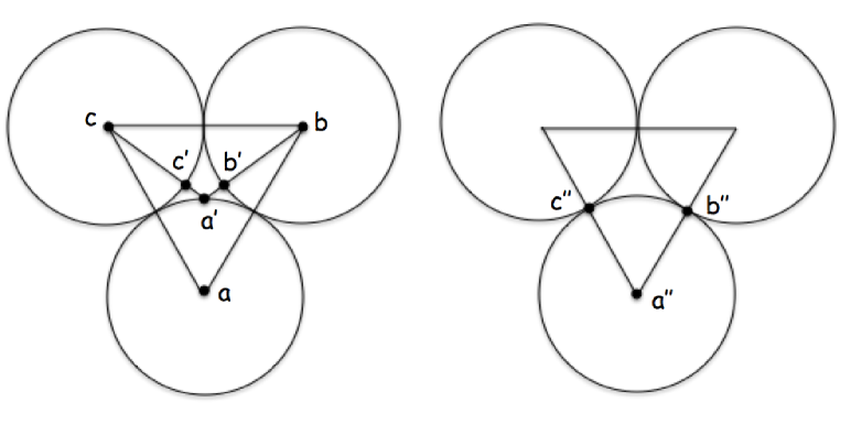
Figure 14: The BCU Problem for three (almost) tangent unit disks. OPT, as shown on the left is given by the choice of locations $(a^{\prime},b^{\prime},c^{\prime})$, not quite on an equilateral triangle, with MBST cost $(\sqrt{1+(\sqrt{3}-1)^{2}}-1)/2\approx.12$, while the “cinch-up” heuristic, on the right, chooses locations $(a^{\prime\prime},b^{\prime\prime},c^{\prime\prime})$ with cost $0.5$.

5 The WCU Problem

We next consider the Worst-Case Connectivity with Uncertainty (WCU) problem: Find the minimum value $\alpha$ such that for any choice of points $P$, the connectivity graph $G_{\alpha}$ of $P$ is connected. In what follows we assume that the number, $n$, of points and associated uncertainty regions is at least $2$, since otherwise the problem is trivial.

We show a simple approximation algorithm for WCU that is within an additive factor of 1 and a multiplicative factor of 2 when the uncertainty regions are unit disks. Let $D(p;\lambda)$ denote the closed disk of radius $\lambda$ about the point $p$.

Theorem 5.1

Given a set of uncertainty regions that are unit disks $D_{1},\ldots,D_{n}$ with centers $p_{1},\ldots,p_{n}$, let $L$ be the largest edge of an MBST on $\{p_{i}:1\leq i\leq n\}$. Then choosing $\alpha=L/2+1$ always results in the connectivity graph being connected and is at worst an OPT$+1$ approximation to the WCU Problem.

Proof

First note that the connectivity graph given by any selection of $\ell_{i}\in D(p_{i};1)$ and $\{D(\ell_{i};L/2+1):1\leq i\leq n\}$ is connected, because if $(p_{i},p_{j})$ is an edge of an MBST on $\{p_{k}:1\leq k\leq n\}$ then $D(\ell_{i};L/2+1)\cap D(\ell_{j};L/2+1)\neq\varnothing$. We are thus left to show that choosing $\alpha=L/2+1$ is at worst an OPT$+1$ approximation. But clearly we can choose $\ell_{i}=p_{i}$ for all $i$ and so the minimum $\alpha$ is $L/2$. Hence OPT $\geq L/2$ and the theorem is established. $\Box$

Theorem 5.2

Given a set of uncertainty regions that are unit disks $D_{1},\ldots,D_{n}$ with centers $p_{1},\ldots,p_{n}$, let $L$ be the largest edge of an MBST on $\{p_{i}:1\leq i\leq n\}$. Then choosing $\alpha=L/2+1$ is at worst a factor $2$ approximation to OPT for the WCU problem.

Proof

Note that OPT$+1\leq 2$OPT as long as OPT $\geq 1$ so, by Theorem 5.1, it suffices to show that OPT $\geq 1$. As noted in the first paragraph of this section we are assuming that $n>1$. Let $p_{j}$ be a leftmost point amongst the $\{p_{i}:1\leq i\leq n\}$ and choose $\ell_{j}$ to be the leftmost point in $D(p_{j};1)$ and for all other $D(p_{k};1)_{k\neq j}$ choose $\ell_{k}$ to be the rightmost point in $D(p_{k};1)$. Then $\ell_{j}$ is at least distance $2$ from each of the other $\ell_{k}$ and so we must choose $\alpha\geq 1$ to keep the connectivity graph connected. It follows that OPT $\geq 1$ and the theorem is established. $\Box$

Theorem 5.2 shows that the simple broadcast-from-center heuristic can be no worse than a $2$-approximation to the solution of the WCU Problem. However, we have thus far only found examples showing that the approximation can be (asymptotically) as bad as a $\sqrt{2}$-approximation, as the next theorem asserts.

Theorem 5.3

Given any $L>2$, there is an instance of the WCU Problem with uncertainty regions that are unit disks $D_{1},\ldots,D_{n}$ with centers $p_{1},\ldots,p_{n}$, such that the longest edge of an MBST on $\{p_{i}\}_{i=1}^{n}$ is $L$ and OPT is as small as $\frac{\sqrt{L^{2}+4}}{2}$, and therefore the algorithm of Theorem 5.1 is at best a factor $\sqrt{2}-\epsilon$ approximation for arbitrarily small $\epsilon$.

Proof

We distribute an even number of unit disks with centers equally spaced along a very large (relative to the unit disks) circle $C$. Let us call the distance between consecutive centers of disks centered along the large circle $L$. We will add more disks, but $L$ will remain the longest edge of a spanning tree of the disk centers. Additionally, let us pick $\epsilon\ll L-2$.

The construction contains a large number of highly overlapping disks in addition to the disks whose centers lie along $C$. See Figure 15 for a sketch.

Figure 15: The construction begins with an even number of equally spaced unit disks with centers along a very large circle $C$.

The drawing is approximate in several respects. First of all, $C$ is much, much larger than drawn, so that if the bottom of $C$ is, say, tangent to the $x$-axis, and the center of the bottom unit disk, $D_{0}$, has $y$-coordinate equal to $0$, then the center-points of the first unit disks to the left and right of $D_{0}$ along $C$, each have $y$-coordinate less than $\epsilon/3$. In addition to the disks along $C$, there is a sequence of disks going from $D_{0}$ to its diametrically opposite unit disk whose centers lie along the connecting diameter. The centers of these disks are all distance $\epsilon$, one from the next, along the diameter. If we number the $C$-centered disks in counter-clockwise order, $D_{0},...,D_{2N-1}$, then we have a similar set of disks extending from each of the disks $D_{2},D_{4},...,D_{2N-2}$. The key observation is that we can add such diametrically centered disks in such a way that the center of disks extending from $D_{j}$ to the center of $C$ are each more than distance $L$ from any other $D_{k}$ for $k\neq j$ – thus the choice of $D_{1}$ and $D_{2N-1}$ with $y$-coordinate less than $\epsilon/3$. On the other hand, the odd numbered unit disks $D_{1},D_{3},...,D_{2N-1}$, with representative element that we shall call $D_{i}$, each have a set of unit disks running from $D_{i}$ to $D_{i+2}$ with centers each $\epsilon$ from the next, but with the disks running in almost circular patterns on the outside of $C$. An important point in this case, is that the disks start out emanating from $D_{i}$ along a diametric line, and then bend around so that their centers are never within $L$ of $D_{i+1}$.

We claim that for such an arrangement of unit disks, the maximum distance between locations $\ell_{r}\in D_{r}$ in a spanning tree can be as small as (and in fact slightly smaller than) $\sqrt{L^{2}+4}$, where the set $\{D_{r}\}$ consists not just of the disks $D_{i}$ with centers along $C$, but all the other unit disks depicted in Figure 15 as well. If $D_{i},D_{i+2}$ are two consecutive disks in the cyclical ordering of $C$-centered disks with $i$ odd, let $\{D_{i_{k}}\}$ denote the set of disks running from $D_{i}$ to $D_{i+2}$ outside of $C$. Further, if $D_{j},D_{j+N}$ are diametrically opposite $C$-centered disks with $j$ even, let $\{D_{j_{k}}\}$ denote the set of disks running diametrically between $D_{j}$ and $D_{j+N}$. To verify our claim about $\{\ell_{i}\}$ with maximum bottleneck spanning tree edge length slightly less than $\sqrt{L^{2}+4}$, pick $\ell_{i}\in D_{i}$ for even $i$ to be the point in $D_{i}$ closest to the center of $C$ and $\ell_{i}\in D_{i}$ for odd $i$ to be the point in $D_{i}$ furthest from the center of $C$. See Figure 16.

Figure 16: The distance between $\ell_{i}$ and $\ell_{i+1}$ (in the cyclical ordering) is just slightly less than $\sqrt{L^{2}+4}$ since the distance between successive disk centers (which we suppose to be x-axis aligned) is $L$, and the distance between the top and bottom of the successive disks, in the y-direction, is approximately $2$.

Regardless of the choice of the $\ell_{i_{j}}\in D_{i_{j}}$ it is clear that $\bigcup\{D(\ell_{i};\alpha)\}~{}\cup~{}\bigcup\{D(\ell_{i_{j}};\alpha)\}$ is connected if $2\alpha$ is the distance between consecutive locations $\ell_{i},\ell_{i+1}$ (in the cyclical ordering), and that this distance is, as claimed, just slightly less than $\sqrt{L^{2}+4}$. Let us designate this distinguished choice of the $\ell_{i}\in D_{i}$ by $\ell_{i}^{*}$, and the associated $\alpha$ by $\alpha^{*}$.

For these $\{D_{i}\}$ and $\{D_{i_{j}}\}$, if there were any choice of $\{\ell_{i}\},\{\ell_{i_{j}}\}$ making $\alpha$ any larger, then we would have to pick one of the $\ell_{i}$ to the left or right of the diametric line through the center of $C$ and $D_{i}$. It is easy to check that the result of such a choice is that there would be some cyclically ordered pair $\ell_{j},\ell_{j+1}$ whose distance $d(\ell_{j},\ell_{j+1})<d(\ell_{j}^{*},\ell_{j+1}^{*})=\alpha^{*}$. But then $D(\ell_{j};\alpha^{*})\cup D(\ell_{j+1};\alpha^{*})$ connects $\ell_{j},\ell_{j+1}$ and $\bigcup\{D(\ell_{2k};\alpha^{*})\}~{}\cup~{}\bigcup\{D(\ell_{(2k)_{j}};\alpha^{*})\}$ connects the even-indexed $\ell_{2k}$ and any associated choices for $\ell_{(2k)_{j}}$, while $\bigcup\{D(\ell_{2k+1};\alpha^{*})\}~{}\cup~{}\bigcup\{D(\ell_{(2k+1)_{j}};\alpha^{*})\}$ connects the odd-indexed $\ell_{2k+1}$ and any associated choices for $\ell_{(2k+1)_{j}}$. It follows that $\alpha\leq\alpha^{*}$, contrary to assumption, and so the fact that OPT can be as small as $\frac{\sqrt{L^{2}+4}}{2}$ is established. The algorithm of Theorem 5.1 picked $\alpha=\frac{L}{2}+1$, so picking $L$ sufficiently close to $2$ yields $\frac{\frac{L}{2}+1}{\frac{\sqrt{L^{2}+4}}{2}}=\frac{L+2}{\sqrt{L^{2}+4}}$ sufficiently close to $\sqrt{2}$, completing the proof. $\Box$

6 Conclusions

A number of open problems remain. It would be interesting to show NP-hardness results for the BCU problem for other uncertainty regions, such as disks. It is also possible that techniques from convex optimization could be used to design approximation algorithms for BCU for, say, line segments or squares. We conjecture that BCU for the case of line segments is W[1]-hard and hence our exact algorithm is unlikely to be improved upon significantly.

Although we have been able to obtain several NP-hardness results for BCU, we do not have any complexity lower bounds for WCU which, a priori, seems harder. It is an interesting open question to improve our approximation algorithms for both these problems.

In conclusion, our work on connectivity problems for uncertainty regions motivated by wireless network scenarios suggests that this area provides a rich collection of problems for further investigation.

References

- [1] M. Abellanas, F. Hurtado, and P. Ramos. Structural tolerance and Delaunay triangulation. Information Processing Letters, 71:221–227, 1999.
- [2] H. Alt, E. Arkin, H. Brönnimann, J. Erickson, S. Fekete, C. Knauer, J. Lenchner, J. Mitchell, and K. Whittlesey. Minimum-cost coverage of point sets by disks. Proceedings of the 22nd ACM Symposium on Computational Geometry (SoCG), pages 449–458, 2006.
- [3] E. M. Arkin, C. Dieckmann, C. Knauer, J. S. B. Mitchell, V. Polishchuk, L. Schlipf, and S. Yang. Convex transversals. In Proceedings of the 12th International Symposium on Algorithms and Data Structures (WADS), pages 49–60, 2011.
- [4] E. M. Arkin and R. Hassin. Approximation algorithms for the geometric covering salesman problem. Discrete Applied Mathematics, 55(3):197–218, 1994.
- [5] E. W. Chambers, A. Erickson, S. P. Fekete, J. Lenchner, J. Sember, V. Srinivasan, U. Stege, S. Stolpner, C. Weibel, and S. Whitesides. Connectivity graphs of uncertainty regions. In 21st International Symposium on Algorithms and Computation (ISAAC), number 5307 in Springer LNCS, pages 434–445, 2010.
- [6] A. E. F. Clementi, P. Penna, and R. Silvestri. On the power assignment problem in radio networks. Technical Report TR00-054, Electronic Colloquium on Computational Complexity, 2000.
- [7] M. de Berg, J. Gudmundsson, M. J. Katz, C. Levcopoulos, M. H. Overmars, and A. F. van der Stappen. TSP with neighborhoods of varying size. Journal of Algorithms, 57(1):22–36, 2005.
- [8] H. Ding and J. Xu. Solving the chromatic cone clustering problem via minimum spanning sphere. In 38th International Colloquium on Automata, Languages and Programming (ICALP), volume 6755 of Springer LNCS, pages 773–784, 2011.
- [9] Y. Disser, M. Mihalák, and S. Montanari. Max shortest path for imprecise points. In 31st European Workshop on Computational Geometry, pages 184–187, 2015.
- [10] Y. Disser, M. Mihalák, S. Montanari, and P. Widmayer. Rectilinear shortest path and rectilinear minimum spanning tree with neighborhoods. In Proceedings of the 3rd International Symposium on Combinatorial Optimization (ISCO), pages 208–220, 2014.
- [11] R. Dorrigiv, R. Fraser, M. He, S. Kamali, A. Kawamura, A. López-Ortiz, and D. Seco. On minimum- and maximum-weight minimum spanning trees with neighborhoods. In Proceedings of the 10th Workshop on Approximation and Online Algorithms (WAOA), pages 93–106, 2012.
- [12] M. Dror, A. Efrat, A. Lubiw, and J. S. B. Mitchell. Touring a sequence of polygons. In Proceedings of the 35th Annual ACM Symposium on Theory of Computing (STOC), pages 473–482, 2003.
- [13] P. Duchet, Y. O. Hamidoune, M. L. Vergnas, and H. Meyniel. Representing a planar graph by vertical lines joining different levels. Discrete Mathematics, 46(3):319–321, 1983.
- [14] A. Dumitrescu and J. S. B. Mitchell. Approximation algorithms for TSP with neighborhoods in the plane. In Proceedings of the 12th ACM-SIAM Symposium on Discrete Algorithms (SODA), pages 38–46, 2001.
- [15] J. Fiala, J. Kratochvíl, and A. Proskurowski. Systems of distant representatives. Discrete Applied Mathematics, 145(2):306–316, 2005.
- [16] B. Fuchs. On the hardness of range assignment problems. In Proceedings of the 6th Italian Conference on Algorithms and Complecity (CIAC), pages 127–138, 2006.
- [17] M. R. Garey and D. S. Johnson. Computers and Intractability: A Guide to the Theory of NP-Completeness. W.H. Freeman, 1979.
- [18] J. Gudmundsson and C. Levcopoulos. A fast approximation algorithm for TSP with neighborhoods. Nordic Journal on Computing, 6(4):469–488, 1999.
- [19] N. Lev-Tov and D. Peleg. Exact algorithms and approximation schemes for base station placement problems. In Proceedings of the 8th Scandinavian Workshop Algorithm Theory (SWAT), pages 90–99, 2002.
- [20] N. Lev-Tov and D. Peleg. Polynomial time approximation schemes for base station coverage with minimum total radii. Computer Networks, 47(4):489–501, 2005.
- [21] D. Lichtenstein. Planar formulae and their uses. SIAM Journal on Computing, 11(2):329–343, 1982.
- [22] M. Löffler and M. van Kreveld. Largest and smallest convex hulls for imprecise points. Algorithmica, 56:235–269, 2010.
- [23] M. Löffler and M. van Kreveld. Largest bounding box, smallest diameter, and related problems on imprecise points. Computational Geometry: Theory and Applications, 43:419–433, 2010.
- [24] C. Mata and J. Mitchell. Approximation algorithms for geometric tour and network design problems. In Proceedings of the 11th ACM Symposium on Computational Geometry (SoCG), pages 360–369, 1995.
- [25] J. S. B. Mitchell. A PTAS for TSP with neighborhoods among fat regions in the plane. In Proceedings of the 18th ACM-SIAM Symposium on Discrete Algorithms (SODA), pages 11–18, 2007.
- [26] X. Pan, F. Li, and R. Klette. Approximate shortest path algorithms for sequences of pairwise disjoint simple polygons. In Proceedings of the 22nd Canadian Conference on Computational Geometry (CCCG), pages 175–178, 2010.
- [27] G. Parker and R. L. Rardin. Guaranteed performance heuristics for the bottleneck traveling salesman problem. Operations Research Letters, 2(6):269 –272, 1984.
- [28] P. Rosenstiehl and R. E. Tarjan. Rectilinear planar layouts and bipolar orientations of planar graphs. Discrete Computational Geometry, 1:343–353, 1986.
- [29] Y. Yang, M. Lin, J. Xu, and Y. Xie. Minimum spanning tree with neighborhoods. In Proceedings of the 3rd Conference on Algorithmic Aspects on Information and Management (AAIM), pages 306–316, Berlin, Heidelberg, 2007. Springer-Verlag.