Transport Processes in Metal-Insulator Granular Layers

Abstract

Tunnel transport processes are considered in a square lattice of metallic nanogranules embedded into insulating host to model tunnel conduction in real metal/insulator granular layers. Based on a simple model with three possible charging states ($\pm$, or $0$) of a granule and three kinetic processes (creation or recombination of a $\pm$ pair, and charge transfer) between neighbor granules, the mean-field kinetic theory is developed. It describes the interplay between charging energy and temperature and between the applied electric field and the Coulomb fields by the non-compensated charge density. The resulting charge and current distributions are found to be essentially different in the free area (FA), between the metallic contacts, or in the contact areas (CA), beneath those contacts. Thus, the steady state dc transport is only compatible with zero charge density and ohmic resistivity in FA, but charge accumulation and non-ohmic behavior are necessary for conduction over CA. The approximate analytic solutions are obtained for characteristic regimes (low or high charge density) of such conduction. The comparison is done with the measurement data on tunnel transport in related experimental systems.

I Introduction

More than three decades have passed since the pioneering studies by Abeles and co-workers sheng1 ; sheng2 that triggered a huge research effort in granular thin films. Actually, nanostructured granular films are of a considerable interest for modern technology due to their peculiar physical properties, like giant magnetoresistance Berk , Coulomb blockade fert ; varalda , or high density magnetic memory park , impossible for continuous materials.

However, a number of related physical mechanisms still needs better understanding, in particular, transport phenomena in these films are still a great challenge and presently various works are addressing such problem beloborodov ; kozub ; ng . The main reason is that granular systems reveals certain characteristics which cannot be obtained neither in the classical conduction regime (in metallic, electrolyte, or gas discharge conduction) nor in the hopping regime (in doped semiconductors or in common tunnel junctions). Their specifics is mainly determined by the drastic difference between the characteristic time of an individual tunneling event ($\sim\hbar/\varepsilon_{\rm F}\sim 10^{-15}$ s) and the interval between such events on the same granule $\sim e/(jd^{2})\sim 10^{-3}$ s, at typical current density $j\sim 10^{-3}$ A/cm² and granule diameter $d\sim 5.0$ nm. Other important moments are the sizeable Coulomb charging energy $E_{c}\sim e^{2}/(\varepsilon_{\rm eff}d)$ (typically $\sim 10$ meV) and the fact that the tunneling rates across the layer may be even several orders of magnitude slower than along it. The interplay of all these factors leads to unusual macroscopic effects, including a peculiar slow relaxation of electric charge discovered in experiments on tunnel conduction through granular layers and granular films Kak1 ; Sch .

For theoretical description of transport processes in granular layers (and multilayers) we develop an extension of the classical Sheng-Abeles model for a single layer of identical spherical particles located in sites of a simple square lattice, with three possible charging states ($\pm$, or $0$) of a granule and three kinetic processes: creation of a $\pm$ pair (the only process included in the original Sheng-Abeles treatment) on neighbor granules, recombination of such a pair, and charge translation from a charged to neighbor neutral granule. Even this rather simple model, neglecting the effects of disorder within a layer and of multilayered structure, reveals a variety of possible kinetic and thermodynamical regimes, well resembling those observed experimentally.

The detailed formulation of the model, its basic parameters, and its mean-field continuum version are given in Sec. II. Next in Sec. III we calculate the mean values of occupation numbers of each charging state under steady state conditions, including the simplest equilibrium situation (no applied fields), in function of temperature. The analysis of current density and related kinetic equation in the out-of-equilibrium case is developed in Sec. IV, where also its simple, ohmic solution is discussed for the FA part of the system. The most non-trivial regimes are found for the CA part, as described in Sec. V for steady state conduction with charge accumulation and non-ohmic behavior. The general integration scheme for non-linear differential equation, corresponding to steady states in FA and CA, and particular approximations leading to their analytic solutions are dropped into Appendix.

II Charging states and kinetic processes

We consider a system of identical spherical metallic nanogranules of diameter $d$, located in sites of simple square lattice of period $a$ within a layer of thickness $b\sim a$ of insulating host with a dielectric constant $\varepsilon$ (Fig. 1).

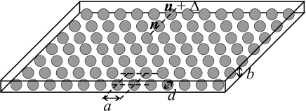
Figure 1: Square lattice of metallic granules in the insulating matrix.

In the charge transfer processes, each granule can bear different numbers $\sigma$ of electrons in excess (or deficit) to the constant number of positive ions and the resulting excess charge $\sigma e$ defines a Coulomb charging energy $\sim\sigma^{2}E_{c}$. At not too high temperatures, $k_{\rm B}T\lesssim E_{c}$, the consideration can be limited only to the ground neutral state $\sigma=0$ and single charged states $\sigma=\pm 1$. Actually, for low metal contents (well separated, small grains), $E_{c}$ reaches $\sim 10-30$ meV, so this approach can be reasonable even above room temperature. For a three-dimensional ($3$D) granular array, $E_{c}$ was defined in the classic paper by Sheng and Abeles sheng1 , under the assumption of a constant ratio between the mean spacing $s$ and granule diameter $d$, in the form $E_{c}=e^{2}f(s/d)/(\varepsilon d)$, where the dimensionless function $f(z)=1/(1+1/2z)$. Otherwise, the complete dielectric response of 3D insulating host with the dielectric constant $\varepsilon$ and metallic particles with the volume fraction $f<1$ and diverging dielectric constant $\varepsilon_{m}\to\infty$ can be characterized by the effective value $\varepsilon_{eff}=\varepsilon/(1-f)$.

For the planar lattice of granules, the analogous effective constant can be estimated, summing the own energy $e^{2}/(\varepsilon d)$ of a charged granule at the ${\bf n}=0$ site and the energy of its interaction with electric dipolar moments $\approx(e/\varepsilon_{eff})(d/2n)^{3}{\bf n}$, induced by the Coulomb field from this charge (in macroscopic dielectric approximation) on all the granules at the sites ${\bf n}=a(n_{1},n_{2})$:

$$E_{c}=\frac{e^{2}}{d}\left[\frac{1}{\varepsilon}-\frac{\alpha}{\varepsilon_{eff}^{2}}\left(\frac{d}{a}\right)^{4}\right]=\frac{e^{2}}{\varepsilon_{eff}d}.$$ (1)

Here the constant $\alpha=\frac{\pi}{4}\sum_{n\neq 0}n^{-4}\approx 5.78$, and the resulting $\varepsilon_{eff}=\left[\varepsilon+\sqrt{\varepsilon^{2}+\varepsilon\alpha(d/a)^{4}}\right]/2>\varepsilon$. However, Eq. 1 may considerably underestimate the most important screening from nearest neighbor granules at $d\sim a$, and in what follows we generally characterize the composite of insulating matrix and metallic granules by a certain $\varepsilon_{eff}=e^{2}/dE_{c}\gg\varepsilon$.

Following the approach proposed earlier Kak1 , we classify the microscopic states of our system, attributing the charging variable $\sigma_{\bf n}$ with values $\pm 1$ or $0$ to each site ${\bf n}$ and then considering three types of kinetic processes between two neighbor granules ${\bf n}$ and ${\bf n}+\Delta$ (Fig. 2):

1. Electron hopping from neutral ${\bf n}$ to neutral ${\bf n}+\Delta$, creating a pair of oppositely charged granules: $(\sigma_{\bf n}=0,\sigma_{{\bf n}+\Delta}=0)\to(\sigma_{\bf n}=+1,\sigma_{{\bf n}+\Delta}=-1)$, only this process was included in the Sheng and Abeles’ theory;

2. Hopping of an extra electron or hole from ${\bf n}$ to neutral ${\bf n}+\Delta$, that is the charge transfer: $(\sigma_{\bf n}=\pm 1,\sigma_{{\bf n}+\Delta}=0)\to(\sigma_{\bf n}=0,\sigma_{{\bf n}+\Delta}=\pm 1)$;

3. Recombination of a electron-hole pair, the inverse to the process 1.: $(\sigma_{\bf n}=+1,\sigma_{{\bf n}+\Delta}=-1)\to(\sigma_{\bf n}=0,\sigma_{{\bf n}+\Delta}=0)$.

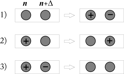
Figure 2: Kinetic processes in a granular layer.

Note that all the processes 1) to 3) are conserving the total system charge $Q=\sum_{{\bf n}}\sigma_{\bf n}$, hence the possibility for charge accumulation or relaxation only appears due to the current leads. A typical configuration for current-in-plane (CIP) tunneling conduction includes two macroscopic metallic electrodes on top of the granular layer, forming contact areas (CA) where the current is being distributed from the electrodes into granules, through an insulating spacer of thickness $b^{\prime}$, and a free area (FA) where the current propagates over the distance $l$ between the contacts (Fig. 3). To begin with, we consider a simpler case of FA while the specific analysis for CA with an account for screening effects by metallic contacts will be given later in Sec. V.

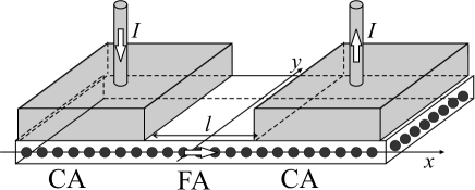
Figure 3: CIP conduction geometry.

The respective transition rates $q_{{\bf n},\Delta}^{(i)}$ for ith process are determined by the instantaneous charging states of two relevant granules and by the local electric field $\mathbf{F}_{\bf n}$ and temperature $T$, accordingly to the expressions:

$$q_{{\bf n},\Delta}^{(1)} = \left(1-\sigma_{{\bf n}}^{2}\right)\left(1-\sigma_{{\bf n}+\Delta}^{2}\right)\varphi\left(e{\mathbf{F}}_{\bf n}\cdot\Delta+E_{c}\right)$$

$$q_{{\bf n},\Delta}^{(2)} = \sigma_{\bf n}^{2}\left(1-\sigma_{{\bf n}+\Delta}^{2}\right)\varphi\left(-e\sigma_{{\bf n}}{\bf F}_{\bf n}\cdot\Delta\right)$$

$$q_{{\bf n},\Delta}^{(3)} = \frac{1}{2}\sigma_{\bf n}\sigma_{{\bf n}+\Delta}\left(\sigma_{\bf n}\sigma_{{\bf n}+\Delta}-1\right)\times$$ (2)

$$\quad\quad\times\,\varphi\left(e\sigma_{{\bf n}+\Delta}{\bf F}_{\bf n}\cdot\Delta-E_{c}\right).$$

Thus the charging energy is positive, $E_{c}$, for the pair creation, zero for the transport, and negative, $-E_{c}$, for the recombination processes. The function $\varphi(E)=\omega N_{\rm F}E/[\exp(\beta E)-1]$ expresses the total probability, at given inverse temperature $\beta=1/(k_{\rm B}T)$, for electron transition between granules with Fermi density of states $N_{\rm F}$ and Fermi levels differing by $E$. The hopping frequency $\omega=\omega_{a}\exp(-2\chi s)$ involves the attempt frequency, $\omega_{a}\sim E_{\rm F}/\hbar$, the inverse tunneling length $\chi$ (typically $\sim 10$ nm^-1), and the inter-granule spacing $s=a-d$. Local electric field ${\bf F}_{\bf n}$ on ${\bf n}$th site consists of the external applied field ${\bf A}$ (site independent) and the Coulomb field ${\bf C}_{\bf n}$ due to all other charges in the system:

$${\bf C}_{\bf n}=\frac{e}{\varepsilon_{eff}}\sum_{{\bf n}^{\prime}\neq{\bf n}}\sigma_{{\bf n}^{\prime}}\frac{{\bf n}^{\prime}-{\bf n}}{\left|{\bf n}^{\prime}-{\bf n}\right|^{3}}.$$ (3)

A suitable approximation is achieved with passing from discrete-valued functions $\sigma_{\bf n}$ of discrete argument ${\bf n}=a(n_{1},n_{2})$ to their continuous-valued mean-field (MF) equivalents $\sigma_{\bf r}=\left\langle\sigma_{\bf n}\right\rangle_{\bf r}$ (mean charge density) and $\rho_{\bf r}=\left\langle\sigma_{\bf n}^{2}\right\rangle_{\bf r}$ (mean charge carrier density). These densities are obtained by averaging over a wide enough area (that is, great compared to the lattice period but small compared to the size of entire system or its parts) around any point ${\bf r}$ in the plane (for simplicity, we drop the position index at averages $\langle\,\rangle_{\bf r}$ in what follows). This also implies passing to a smooth local field:

$${\bf F}_{\bf r}={\bf A}+\frac{e}{\varepsilon_{eff}a^{2}}\int\sigma({\bf r}^{\prime})\frac{{\bf r}^{\prime}-{\bf r}}{|{\bf r}^{\prime}-{\bf r}|^{3}}d{\bf r}^{\prime}.$$ (4)

and to the averaged transition rates $q^{(i)}_{{\bf r},\Delta}=\left\langle q_{{\bf n},\Delta}^{(i)}\right\rangle$ and $p^{(i)}_{{\bf r},\Delta}=\left\langle\sigma_{\bf n}q_{{\bf n},\Delta}^{(i)}\right\rangle$. These rates fully define the temporal derivatives of mean densities:

$$\dot{\sigma}_{\bf r} = \sum_{\Delta}\left[q^{(1)}_{{\bf r},\Delta}-q^{(1)}_{{\bf r}+\Delta,-\Delta}-p^{(2)}_{{\bf r},\Delta}+p^{(2)}_{{\bf r}+\Delta,-\Delta}\right.$$ (5)

$$\qquad\qquad\qquad\qquad\qquad\qquad\qquad-\left.p^{(3)}_{{\bf r},\Delta}\right],$$

$$\dot{\rho}_{\bf r} = \sum_{\Delta}\left[q^{(1)}_{{\bf r},\Delta}+q^{(1)}_{{\bf r}+\Delta,-\Delta}-q^{(2)}_{{\bf r},\Delta}+q^{(2)}_{{\bf r}+\Delta,-\Delta}\right.$$ (6)

$$\qquad\qquad\qquad\qquad\qquad\qquad\qquad-\left.q^{(3)}_{{\bf r},\Delta}\right].$$

The set of Eqs. 2-6 provides a continuous description of the considered system, once a proper averaging procedure is established.

III Mean-field densities in equilibrium

We perform the above defined averages in the simplest assumption of no correlations between different sites: $\left\langle f_{\bf n}g_{{\bf n}^{\prime}}\right\rangle=\left\langle f_{\bf n}\right\rangle\left\langle g_{{\bf n}^{\prime}}\right\rangle$, ${\bf n}^{\prime}\neq{\bf n}$, and using the evident rules: $\left\langle\sigma_{\bf n}^{2k+1}\right\rangle=\sigma_{\bf r}$, $\left\langle\sigma_{\bf n}^{2k}\right\rangle=\rho_{\bf r}$. The resulting averaged rates are:

$$q^{(1)}_{{\bf r},\Delta} = \sigma^{0}_{\bf r}\sigma^{0}_{{\bf r}+\Delta}\varphi\left(e{\bf F}_{\bf r}\cdot\Delta+E_{c}\right),$$

$$q^{(2)}_{{\bf r},\Delta} = \sigma^{0}_{{\bf r}+\Delta}\left[\sigma^{+}_{\bf r}\varphi\left(-e{\bf F}_{\bf r}\cdot\Delta\right)\right.$$

$$\qquad\qquad\qquad+\left.\sigma^{-}_{\bf r}\varphi\left(e{\bf F}_{\bf r}\cdot\Delta\right)\right],$$

$$p^{(2)}_{{\bf r},\Delta} = \sigma^{0}_{{\bf r}+\Delta}\left[\sigma^{+}_{\bf r}\varphi\left(-e{\bf F}_{\bf r}\cdot\Delta\right)\right.$$

$$\qquad\qquad\qquad-\left.\sigma^{-}_{\bf r}\varphi\left(e{\bf F}_{\bf r}\cdot\Delta\right)\right],$$

$$q^{(3)}_{{\bf r},\Delta} = \left[\sigma^{+}_{\bf r}\sigma^{-}_{{\bf r}+\Delta}\varphi\left(-e{\bf F}_{\bf r}\cdot\Delta-E_{c}\right)\right.$$

$$\qquad+\left.\sigma^{-}_{\bf r}\sigma^{+}_{{\bf r}+\Delta}\varphi\left(e{\bf F}_{\bf r}\cdot\Delta-E_{c}\right)\right],$$

$$p^{(3)}_{{\bf r},\Delta} = \left[\sigma^{+}_{\bf r}\sigma^{-}_{{\bf r}+\Delta}\varphi\left(-e{\bf F}_{\bf r}\cdot\Delta-E_{c}\right)\right.$$ (7)

$$\qquad\qquad-\left.\sigma^{-}_{\bf r}\sigma^{+}_{{\bf r}+\Delta}\varphi\left(e{\bf F}_{\bf r}\cdot\Delta-E_{c}\right)\right],$$

where the mean occupation numbers for each charging state $\sigma^{\pm}_{\bf r}=(\rho_{\bf r}\pm\sigma_{\bf r})/2$ and $\sigma^{0}_{\bf r}=1-\rho_{\bf r}$ satisfy the normalization condition: $\sum_{i}\sigma^{i}_{\bf r}=1$.

In a similar way to Eq. 5, we express the vector of average current density ${\bf j}_{\bf n}$ at ${\bf n}$th site:

$${\bf j}_{\bf n} = \frac{e}{a^{2}b}\sum_{\Delta}\Delta\left[-q^{(1)}_{{\bf n},\Delta}+q^{(1)}_{{\bf n}+\Delta,-\Delta}\right.$$ (8)

$$+ \left.p^{(2)}_{{\bf n},\Delta}-p^{(2)}_{{\bf n}+\Delta,-\Delta}+p^{(3)}_{{\bf n},\Delta}\right],$$

and then its MF extension $\bf{j}_{\bf r}$ is obtained by simple replacing ${\bf n}$ by ${\bf r}$ in the arguments of $q^{(i)}$ and $p^{(i)}$. Expanding these continuous functions in powers of $|\Delta|=a$, we conclude that Eq. 5 gets reduced to usual continuity equation:

$$\dot{\sigma}_{\bf r}=-\frac{a^{2}b}{e}\nabla_{2}\cdot\bf{j}_{\bf r},$$ (9)

with the two dimensional ($2$D) nabla: $\nabla_{2}=(\partial_{x},\partial_{y})$. We begin the analysis of Eqs. 5 - 9 from the simplest situation of thermal equilibrium in absence of electric field, $\bf{F_{r}}\equiv 0$, then Eq. 5 turns into evident identity: $\sigma_{\bf r}\equiv 0$, that means zero charge density, and Eq. 8 yields in zero current density: ${\bf j}_{\bf r}\equiv 0$, while Eq. 6 provides a finite and constant value of charge carrier density:

$$\rho_{\bf r}\equiv\rho_{e}=\frac{2}{2+\exp\left(\beta E_{c}/2\right)}.$$ (10)

At low temperatures, $\beta E_{c}\gg 1$, this value is exponentially small: $\rho_{e}\approx 2\exp(-\beta E_{c}/2)$, and for high temperatures, $\beta E_{c}\ll 1$, it behaves as $\rho_{e}\approx\rho_{\infty}-\beta E_{c}/9$, tending to the limit $\rho_{\infty}=2/3$, corresponding to equipartition between all three fractions $\sigma^{i}$ (Fig. 4, though this limit being beyond actual validity of the model, as indicated in Sec. II).

Figure 4: Equilibrium density $\rho_{e}$ of charge carriers in function of temperature (solid line). The curve $1$ (dashed line) corresponds to the low temperature asymptotics $\rho_{e}\approx 2\exp\left(-E_{c}/2k_{\rm B}T\right)$, and the curve 2 (dash-dotted line) to the high temperature asymptotic $\rho_{e}\approx\rho_{\infty}-E_{c}/9k_{\rm B}T$, converging to the limit $\rho_{\infty}=2/3$ (dotted line).

In presence of electric fields ${\bf F}_{\bf r}\neq 0$, the local equilibrium should be perturbed and the system should generate current and generally accumulate charge. Then, from Eq. 6, the charge density $\sigma_{\bf r}$ is related to the carrier density $\rho_{\bf r}$ as:

$$\sigma^{2}_{\bf r}=\frac{\left(\rho_{\bf r}-\rho_{e}\right)\left(\rho_{\bf r}+\rho_{e}-2\rho_{e}\rho_{\bf r}\right)}{\left(1-\rho_{e}\right)^{2}},$$ (11)

describing the increase of charge density with going away from equilibrium. As seen from Fig. 5, for not too high temperatures $T\lesssim E_{c}/k_{\rm B}$ where the neglect of multiple charged states is justified, this dependence is reasonably close to the simplest low-temperature form:

$$\sigma\approx\sqrt{\rho^{2}-\rho_{e}^{2}},$$ (12)

that will be practically used in what follows.

Now we are in position to pass to the out-of-equilibrium situations, beginning from a simpler case of dc current flowing through the FA.

Figure 5: The charge density $\sigma$ in function of the carrier density $\rho$ for different temperatures (corresponding to different thermal equilibrium values $\rho_{e}$). Note closeness of all the curves to that for low-temperature limit $\rho_{e}\to 0$, given exactly by Eq. 12.

IV Steady state conduction in FA

In presence of (generally non-uniform) fields ${\bf F}_{\bf r}$ and densities $\sigma_{\bf r}$, $\rho_{\bf r}$, we expand Eq. 8 up to 1st order terms in $|\Delta|=a$ and obtain the local current density as a sum of two contributions, the field-driven and diffusive:

$${\bf j}_{\bf r}={\bf j}^{\rm field}_{\bf r}+{\bf j}^{\rm dif}_{\bf r}=g\left(\rho_{\bf r}\right){\bf F}_{\bf r}-eD\left(\rho_{\bf r}\right)\nabla_{2}\sigma_{\bf r},$$ (13)

where the effective conductivity $g$ and diffusion coefficient $D$ are functions of the local charge carrier density, $\rho\equiv\rho_{\bf r}$:

$$g(\rho) = \frac{e^{2}}{b}\left|\frac{}{}2(1-\rho)^{2}\varphi^{\prime}\left(E_{c}\right)+\rho(1-\rho)\varphi^{\prime}(0)\right.$$

$$+ \left.\frac{1}{2}(\rho^{2}-\sigma^{2})\varphi^{\prime}\left(-E_{c}\right)\right|,$$

$$D(\rho) = \frac{\rho(1-\rho_{e})^{2}\varphi(0)(1-\rho)\rho_{e}^{2}\varphi(-E_{c})/2}{\rho(1-2\rho_{e})+\rho_{e}^{2}}.$$ (14)

In view of Eqs. 11, 12, we can consider $g$ and $D$ as even functions of local charge density $\sigma$, and just this dependence will be mostly used below. Also $g$ and $D$ depend on temperature, through the functions $\varphi$ and $\varphi^{\prime}$. The system of Eqs. 11 -14, together with Eq. 4, is closed and self-consistent, defining the distributions of $\sigma_{\bf r}$ and $\rho_{\bf r}$ at given ${\bf j}_{\bf r}$. It is readily seen to admit the trivial solution, $\sigma(x)\equiv 0$, and now we shall argue that in fact this is the only practical solution for FA.

First of all, we notice physical restrictions on the charge accumulation in FA. By the problem symmetry, the charge density should only depend on the coordinate along the current, $\sigma=\sigma(x)$, this function being odd (in the geometry of Fig. 3) and supposedly monotonous. Then its maximum value $\sigma_{\rm max}=\sigma(L/2)$ will define the characteristic scale for the Coulomb field: $C\sim\sigma_{\rm max}e/\left(\varepsilon_{\rm eff}a^{2}\right)$ which should not be higher than typical applied fields $A\sim 10^{2}$ V/cm (as seen from relatively moderate non-ohmic vs ohmic response in the experiment). Thus the maximum charge density should not surpass the level of $A\varepsilon_{\rm eff}a^{2}/e\sim 10^{-3}$, that is much lower than the equilibrium density of charge carriers $\rho_{e}$ (except for, maybe, too low temperatures, $T\lesssim 0.07E_{c}/k_{\rm B}\sim 10$ K). Therefore, one can neglect the small difference, Eq. 12, setting constant values: $\rho\approx\rho_{e}$ and then $g\approx g_{e}\equiv g(\rho_{e}),\,D\approx D_{e}\equiv D(\rho_{e})$.

Under such condition, we can eliminate the (not well known) constant $A$ from Eq. 13, bringing this equation to the integro-differential form:

$$\frac{\partial^{2}\sigma(x)}{\partial x^{2}}=\frac{g_{e}}{D_{e}\varepsilon_{\rm eff}a^{2}}P\int_{-l/2}^{l/2}\frac{\sigma(x^{\prime})dx^{\prime}}{(x-x^{\prime})^{2}},$$ (15)

where the $P$-symbol at integration in $x^{\prime}$ means the "discrete principal value", that is omission of the interval $(x-a,x+a)$ to avoid the apparent divergence, in agreement with the minimum distance between granules in the lattice. Thus the regularized integral converges rapidly, then it is reasonable to fix the argument of $\sigma$-density at $x^{\prime}=x$, arriving at a simple differential equation:

$$\frac{\partial^{2}\sigma(x)}{\partial x^{2}}=\frac{\sigma(x)}{r_{\beta}^{2}}.$$ (16)

Here the parameter

$$r_{\beta}^{2}=\frac{a^{3}}{d}\frac{2{\rm e}^{\beta E_{c}}+5{\rm e}^{\beta E_{c}/2}+2}{{\rm e}^{3\beta E_{c}/2}+2\beta E_{c}{\rm e}^{\beta E_{c}}-{\rm e}^{\beta E_{c}/2}}$$

defines the temperature dependent length scale $r_{\beta}$, and the $x$-odd solution of Eq. 16 is just $\sigma(x)=\sigma_{1}\sinh(x/r_{\beta})$. However, for all the considered temperatures, $\beta E_{c}\gtrsim 1$ (see the note in Sec. II), this scale is $r_{\beta}\lesssim a$, that is by many orders of magnitude smaller than the FA size $l$. Then the estimate for the constant $\sigma_{1}$ in the above solution, $\sigma_{1}\sim\sigma_{\rm max}{\rm e}^{-l/r_{\beta}}$ with the exponent as great as for instance $l/r_{\beta}\sim 10^{4}$, makes this solution practically vanishing within whole FA, except maybe for a very narrow vicinity $\sim r_{\beta}$ of its interface with CA (where, strictly speaking, Eq. 16 no more holds). This evident consequence of long-range character of Coulomb fields in FA will be contrasted below with the situation in CA, where charge accumulation turns possible due to screening effects by the metallic contacts and to the related short-range fields.

Thus we conclude that there is practically no charge accumulation and hence no diffusive contribution to the current in FA. Thus the steady state of FA in out-of-equilibrium conditions should be characterized by the ohmic conductivity $g_{e}$. In fact, an estimation (based on an experimental system silva ) suggests that the FA contribution to the overall resistance turns to be about two orders of magnitude smaller than the CA one (see below), and thus the transport is expected to be mainly controlled by CA.

V Steady state conduction in CA

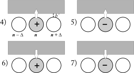
Figure 6: Kinetic processes between ${\bf n}$th granule and the metallic electrode in CA.

The kinetics in CA includes, besides the processes 1) to 3) of Sec. III and IV, also four additional microscopic processes between ${\bf n}$th granule and the electrode (Fig. 6) which are just responsible for variations of total charge $Q$ by $\pm 1$. The respective rates $q^{(i)}$, $i=4,\ldots 7$, are also dependent on the charging state $(\sigma_{\bf r},\rho_{\bf r})$ of the relevant granule and, using the same techniques that before, their mean values are:

$$q^{(4)}_{\bf r} = \left(\rho_{\bf r}+\sigma_{\bf r}\right)\psi(-U-E_{c}^{\prime}),$$

$$q^{(5)}_{\bf r} = \left(\rho_{\bf r}-\sigma_{\bf r}\right)\psi\left(U-E_{c}^{\prime}\right),$$

$$q^{(6)}_{\bf r} = \left(1-\rho_{\bf r}\right)\psi\left(U+E_{c}^{\prime}\right),$$

$$q^{(7)}_{\bf r} = \left(1-\rho_{\bf r}\right)\psi\left(-U+E_{c}^{\prime}\right).$$ (17)

Here the function $\psi(E)$ formally differs from $\varphi(E)$ only by changing the pre-factor: $\omega\to\omega^{\prime}=\omega_{a}{\rm e}^{-2\chi b^{\prime}}\ll\omega$, but the arguments of these functions in Eq. 17 include other characteristic energies. Thus, the energy $U=eb^{\prime}S$ is due to the electric field $S\equiv F_{c}(z=b^{\prime})$ at the contact surface above the granule. As seen from Fig. 7, this field is always normal to the surface and its value is defined by the local charge density $\sigma$ (see below). At least, the charging energy $E_{c}^{\prime}$ for a granule under the contact can be somewhat lower (e.g., by $\sim 1/2$) than $E_{c}$. Then the kinetic equations in interface region present a generalization of Eqs. 5-6, as follows:

$$\dot{\sigma}_{\bf r} = \sum_{{\Delta}}\left[q^{(1)}_{{\bf r},\Delta}-q^{(1)}_{{\bf r}+\Delta,-\Delta}-p^{(2)}_{{\bf r},\Delta}+p^{\left(2\right)}_{{\bf r}+\Delta,-\Delta}-p^{(3)}_{{\bf r},\Delta}\right.$$ (18)

$$\left.\quad\quad\quad-q^{(4)}_{\bf r}+q^{(5)}_{\bf r}+q^{(6)}_{\bf r}-q^{(7)}_{\bf r}\right],$$

$$\dot{\rho}_{\bf r} = \sum_{\Delta}\left[q^{(1)}_{{\bf r},\Delta}+q^{(1)}_{{\bf r}+\Delta,-\Delta}-q^{(2)}_{{\bf r},\Delta}+q^{(2)}_{{\bf r}+\Delta,-\Delta}-q^{(3)}_{{\bf r},\Delta}\right.$$ (19)

$$\left.\quad\quad\quad-q^{(4)}_{\bf r}-q^{(5)}_{\bf r}+q^{(6)}_{\bf r}+q^{(7)}_{\bf r}\right].$$

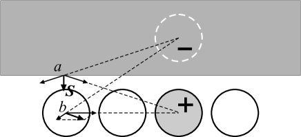
Figure 7: Formation of local electrical fields by a dipole of a charged granule and its (oppositely charged) image: at the surface of the metallic electrode (point a) and on other granule (point b).

The additional terms, by the normal processes 4) to 7), are responsible for appearance of a normal component of current density:

$$j^{z}_{\bf r}=\frac{e}{a^{2}}\left[q^{(4)}_{\bf r}-q^{(5)}_{\bf r}-q^{(6)}_{\bf r}+q^{(7)}_{\bf r}\right],$$ (20)

besides the planar component, still given by Eq. 8. But an even more important difference from the FA case is the fact that the Coulomb field here is formed by a double layer of charges, those by granules themselves and by their images in the metallic electrode (Fig. 7). Summing the contributions from all the charged granules and their images (except for the image of ${\bf n}$th granule itself, already included in the energy $E_{c}^{\prime}$), we find that the above mentioned field at the contact surface above the point ${\bf r}$ of the granular layer, $S_{\bf r}$, can be expressed as a local function of the charge density $\sigma_{\bf r}$:

$$S_{\bf r}=C_{\bf r}(z=b^{\prime})=-\frac{4\pi e}{\varepsilon a^{2}}\sigma_{\bf r},$$ (21)

replacing the integral relations, Eqs. 3-4, in FA. Also, note that the relevant dielectric constant for this field formed outside the granular layer is rather the host value $\varepsilon$ than the renormalized $\varepsilon_{eff}$ within the layer (as by Eq. 3). Then, the planar component of the field by charged granules ${\bf F}^{pl}_{\bf r}={\bf C}_{\bf r}(z=0)$ is determined by the above defined normal field $S_{\bf r}$ through the relation ${\bf F}^{pl}_{\bf r}=b^{\prime}\nabla_{2}S_{\bf r}$. The density of planar current is ${\bf j}^{pl}_{\bf r}=g{\bf F}^{pl}_{\bf r}-eD{\nabla}_{2}\sigma_{\bf r}$, accordingly to Eq. 13, that is both field-driven and diffusive contributions into ${\bf j}^{pl}_{\bf r}$ are present here and both they are proportional to the gradient of $\sigma_{\bf r}$. In the low temperature limit, this proportionality is given by:

$${\bf j}^{pl}_{\bf r}\approx-\left[\frac{8\pi e^{3}\omega N_{\rm F}b^{\prime}}{\varepsilon_{eff}a^{3}}g\left(\sigma_{\bf r}\right)+\frac{e\omega N_{\rm F}k_{\rm B}T}{a}\right]\nabla_{2}\sigma_{\bf r}.$$ (22)

Note that the presence of a non-linear function:

$$g(\sigma)=\sqrt{\rho_{e}^{2}+\sigma^{2}}-2\rho_{e}^{2}-\sigma^{2},$$

defines a non-ohmic conduction in CA. In fact, this function should be defined by Eq. 21 only for charge density below its maximum possible value $|\sigma_{max}|=\sqrt{1-\rho_{e}^{2}}$, turning zero for $|\sigma|>|\sigma_{max}|$ (note that the latter restriction just corresponds to our initial limitation to the single charged states, see Sec. II). In the same limit of low temperatures, the normal current density is obtained from Eqs. 16, 17 as ${\bf j}_{z}({\bf r})=G_{z}\Sigma_{\bf r}$ where $G_{z}\approx\omega^{\prime}N_{\rm F}E^{\prime}_{c}\varepsilon_{eff}/4\pi$. Finally, the kinetic equation in this case is obtained, in analogy with Eq. 8, as:

$$\dot{\sigma}_{\bf r}=-\frac{a^{2}b}{e}\nabla_{2}\cdot{\bf j}^{pl}_{\bf r}+\frac{a^{2}}{e}j^{z}_{\bf r}.$$ (23)

This equation permits to describe the steady state conduction as well as various time dependent processes. The first important conclusion is that steady state conduction in the interface turns only possible at non-zero charge density gradient, that is, necessarily involving charge accumulation, in contrast to the above considered situation in bulk.

Let us restrict here the analysis to the steady state conduction regime which is simpler, though the obtained results can be also used for the analysis of a more involved case when an explicit temporal dependence of charge density is included in Eq. 23 (this will be a topic of future study).

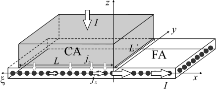
Figure 8: Relations between longitudinal ($j_{x}$) and normal ($j_{z}$) currents in CA, adding to the total current $I$.

We choose the contacts geometry in the form of a rectangular stripe of planar dimensions $L\times L^{\prime}$, along and across the current respectively. In neglect of relatively small effects of current non-uniformity along the lateral boundaries, the only relevant coordinate for the problem is longitudinal, $x$ (Fig. 8), so we consider the relevant function $\sigma_{x}$ with its derivatives, spatial $\sigma_{x}^{\prime}$ and temporal $\dot{\sigma_{x}}$. In the steady state regime, $\dot{\sigma}=0$ in Eq. 23, and the total current $I=\rm{const}$, defined by the action of external source. Then, using the above approximation for $g(\sigma)$, a non-linear 2nd order equation for charge density is found:

$$\frac{d}{dx}\left\{\left[g\left(\sigma_{x}\right)+\tau\right]\sigma_{x}^{\prime}\right\}-k^{2}\sigma_{x}=0.$$ (24)

Here the parameters are: $k^{2}=(\omega^{\prime}E_{c}^{\prime})/\left(ab\omega k_{\rm B}T_{1}\right)$ and $\tau=T/T_{1}$, where $T$ is the actual temperature and $T_{1}=8\pi e^{2}b^{\prime}/a^{2}k_{\rm B}\varepsilon_{eff}$. To define completely its solution, the following boundary conditions are imposed:

$$\sigma_{x=0}^{\prime}=\frac{k^{2}b^{\prime}\sigma_{x=0}}{g\left(\sigma_{x=0}\right)+\tau},$$ (25)

$$\sigma_{x=L}^{\prime}=\frac{a}{Le\omega bN_{\rm F}k_{\rm B}T_{1}}\frac{I}{g\left(\sigma_{x=L}\right)+\tau}.$$ (26)

Here Eq. 25 corresponds to the fact that the longitudinal current $j^{x}$ at the initial point of contact/granular sample interface (the leftmost in Fig. 8) is fully supplied by the normal current $j^{z}$ entering from the contact to the granular sample, and Eq. 26 corresponds to the current continuity at passage from CA (of length $L$ along the $x$ axis) to FA.

Let us discuss the solution of Eq. 24 qualitatively. Generally, to fulfill the conditions, Eqs. 25, 26, one needs a quite subtle balance to be maintained between the charge density and its derivatives at both ends of contact interface. But the situation is radically simplified when the length $L$ is much greater than the characteristic decay length for charge and current density: $kL\gg 1$. In this case, the relevant coordinate is $\xi=L-x$, so that the boundary condition 25 corresponds to $\xi=L\to\infty$, when both its left and right hand side turn zeros:

$$\sigma_{\xi\to\infty}=0,\qquad\sigma_{\xi\to\infty}^{\prime}=0.$$ (27)

The numeric solution shows that, for any initial (with respect to $\xi$, that is related to $x=L$, Eq. 26) value of charge density $\sigma_{\xi=0}=\sigma_{0}$, there is a unique initial value of its derivative $\sigma_{\xi=0}^{\prime}=D(\sigma_{0})$ which just assures the limits, Eq. 27, while for $\sigma_{\xi=0}^{\prime}>D(\sigma_{0})$ the asymptotic value diverges as $\sigma_{\xi\to\infty}\to\infty$, and for $\sigma_{\xi=0}^{\prime}<D(\sigma_{0})$ it diverges as $\sigma_{\xi\to\infty}\to-\infty$. Then, using the boundary condition, Eq. 26, and taking into account the relation $V=V_{0}\sigma_{0}$ following from Eq. 23 with $V_{0}=4\pi eb^{\prime}/(\varepsilon_{eff}a^{2})$, we conclude that the function $D(\sigma_{0})$ generates the I-V characteristics:

$$I=I_{1}b^{\prime}D\left(\frac{V}{V_{0}}\right)\left[g\left(\frac{V}{V_{0}}\right)+\tau\right],$$ (28)

where $I_{1}=e\omega N_{\rm F}k_{\rm B}T_{1}$.

A more detailed analysis of Eq. 24 is presented in Appendix. In particular, for the weak current regime (Regime I) when $\sigma_{0}\ll\sigma_{1}=\sqrt{32\rho_{e}(\rho_{e}+\tau)}\ll 1$, so that $g(\sigma)\approx\rho_{e}+\sigma^{2}/\left(2\rho_{e}\right)$ along whole the contact interfaces, Eq. 23 admits an approximate analytic solution:

$$\sigma_{\xi}=\sigma_{0}{\rm e}^{-\lambda\xi}\left[1+6\left(\frac{\sigma_{0}}{\sigma_{1}}\right)^{2}\left(1-{\rm e}^{-2\lambda\xi}\right)\right],$$ (29)

with the exponential decay index $\lambda=k/\sqrt{\rho_{e}+\tau}$.

This results in the explicit I-V characteristics for Regime I:

$$I=G_{0}V\left[1+\left(\frac{V}{V_{1}}\right)^{2}\right],$$ (30)

for $V<V_{1}=\sigma_{1}V_{0}$, Eq. 30 describes the initial ohmic CA conductance (temperature $\tau$ dependent):

$$G_{0}=\frac{I_{1}kb^{\prime}}{V_{0}}\sqrt{\rho_{e}\left(\tau\right)+\tau},$$ (31)

which turns non-ohmic for $V\sim V_{1}$. But at so high voltages another conduction regime already applies (called Regime II), where $\sigma_{1}\ll\sigma_{0}\ll 1$ and one has $g(\sigma)\approx\sigma$ (see Eq. 21). Following the same reasoning as for the Regime I, we obtain a non-linear I-V characteristics for Regime II:

$$I\approx\frac{I_{1}kb^{\prime}}{\sqrt{3V_{0}^{3}}}\left(V+V_{0}\tau\right)^{3/2}$$ (32)

this law is weaker temperature dependent than Eq. 30, which is related to the fact that the conductance in Regime II is mainly due to dynamical accumulation of charge and not to thermic excitation of charge carriers. Interestingly a $I\propto V^{3/2}$ law was recently found in experimental measurements silva . Further, such non-linearity can be yet more pronounced if multiple charging states are engaged, as may be the case in real granular layers with a certain statistical distribution of granule sizes present.

At least, for even stronger currents, when already $\sigma_{0}\sim 1$, the solutions of Eq. 24 can be obtained numerically, following the above discussed procedure of adjustment of the derivative $D(\sigma_{0})$ to a given $\sigma_{0}$. Such solutions have an asymptotic behavior of the type: $I\propto V^{5/4}$.

A simple and important exact relation for the total accumulated charge $Q$ in CA is obtained from the direct integration of Eq. 24:

$$Q=tI,$$

where the parameter $t=1/\psi\left(-E_{c}^{\prime}\right)$ should have a role of characteristic relaxation time in non-stationary processes. Assuming its value $t\sim 1$ s (comparable with the experimental observations Kak1 ), together with the above used values of $\omega$ and $T_{1}$, we conclude that the characteristic length scale $\lambda^{-1}$ for solutions of Eq. 24 can reach up to $\sim 10^{3}a\sim 1\mu$m, which is a reasonable scale for a charge distribution beneath the contacts.

VI Global conduction in the system

The conduction in the overall system results from matching of the above considered processes in CA and FA. Thus, in order to evaluate the global resistance of this circuit in series it is necessary to add the contributions of both areas to it. Recent measurements silva have shown notably non-linear I-V curves (already at low enough voltages), so, accordingly to the above discussion, this indicates that the resistance should be dominated by CA. To have a clear view on it, we can use the typical parameters for the granular film: $a\sim 5$ nm, $d\sim 4$ nm, $\chi\sim 10$ nm^-1, $b\sim 8$ nm, $b^{\prime}\sim 2$ nm, $E_{c}\sim 10$ meV, $N_{F}\sim 1$ eV^-1 and take $\omega$ as a (less known) fitting parameter. For the considered rectangular CIP geometry we also use the experimental values silva of width $L^{\prime}=3$ mm and of distance between the contacts $l=100$ $\mu$m.

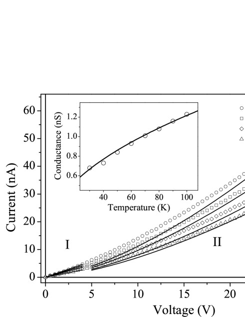
Figure 9: I-V characteristics for a granular sample at different temperatures, compared with the theoretical curves for for regimes I and II. Inset: temperature dependence of ohmic conductance $G_{0}$, measured data (circles) vs calculated by Eq. 31.

Choosing $T=50$ K, the ohmic conductance of the FA, $G_{FA}$, can be calculated through the formula $G_{FA}=g(\rho_{e})L^{\prime}b/l\approx\omega\,1.5\times 10^{-18}$ S. In the CA, we can estimate the conductance (in Regime I) following the above formula $G_{CA}\approx\omega\,8.0\times 10^{-22}$ S. Thus it is clear that, for any choice of $\omega$, the conductance of the CA is about 4 orders of magnitude smaller than that of the FA and for that reason it should dominate the global resistance of the system. Then, using the formulae, Eqs. 29-31, we obtain a good agreement with the experimental data by Ref. silva as shown in Fig. 9. It should be noted however that the effective value of the parameter $V_{0}$ giving the best fit to the experimental data should be notably higher then that given by our formula (before Eq. 28) for single layer system. Thus, with the above choice of other parameters, we have the single-layer value $V_{0}\approx 0.5$ V whereas the best fit for 10-layer experimental sample needs instead $V_{exp}\approx 3$ V. This difference can be effectively accounted for by a simple multiplicative factor $\alpha\approx 6$ (the "multilayer factor") so that $V_{exp}=\alpha V_{0}$ assures both the agreement for Regimes I,II of I-V curves and the boundary $V\sim V_{exp}$ between them, clearly seen in Fig 9.

VII Conclusion

In conclusion, the mean-field model is developed for tunnel conduction in a granular layer, including three principal processes of creation and annihilation of pairs of opposite charges on neighbor granules and of charge transfer from a charged granule to a neighbor neutral granule. Effective kinetic equations for averaged charge densities are derived for the characteristic areas of the granular sample: the contact areas beneath metallic current leads and free area between these leads. From these kinetic equations, it is shown that the tunnel conduction in the free area does not produce any notable charge accumulation, and the conduction regime here is purely ohmic. Contrariwise, such conduction in the contact area turns impossible without charge accumulation, leading to generally non-ohmic conduction regime, since the contact area dominates in the overall resistance. Approximate analytic treatment is developed for calculation of charge density and tunnel current in two characteristic regimes: I) for weak charge accumulation (compared to the thermal density of charge carriers) and II) for strong charge accumulation, leading to a non-ohmic $I\propto V^{3/2}$ conduction law. The calculated I-V curves and temperature dependencies are found in a good agreement with available experimental data. The proposed model can be further developed for description of multilayer strucuture effects and also of non-stationary conduction processes, like anomalous slow current relaxation Kak2 . Finally, the elastic effects of Coulomb forces by charged granules can be included in order to explain the remarkable phenomenon of resistive-capacitive switching silva2 , in granular layered conductors.

VIII Acknowledgements

The authors are grateful to G.N. Kakazei, J.A.M. Santos, J.B. Sousa, J.P. Araújo, J.M.B. Lopes dos Santos and H.L. Gomes for kind assistance and valuable help in various parts of this work. One of us (HGS) gratefully acknowledges the support from Portuguese FCT through the grant SFRH/BPD/63880/2009.

IX Appendix

Let us consider the equation:

$$\frac{d}{d\xi}\left[g(\sigma)+\tau\right]\frac{d\sigma}{d\xi}-k^{2}\sigma=0$$ (A1)

with certain boundary conditions $\sigma(0)=\sigma_{0}$, $\sigma^{\prime}(0)=\sigma_{0}^{\prime}$, resulting from Eqs. 24, 25. For a rather general function $g(\sigma)$ we can define the function

$$f(\sigma)=\int_{0}^{\sigma}g(\sigma^{\prime})d\sigma^{\prime},$$ (A2)

then Eq. A1 presents itself as:

$$\frac{d^{2}F_{\xi}}{d\xi^{2}}=k^{2}\sigma_{\xi},$$ (A3)

where $F_{\xi}\equiv f\left(\sigma_{\xi}\right)+\tau\sigma_{\xi}$. Considered irrespectively of $\xi$:

$$f(\sigma)+\tau\sigma=F,$$ (A4)

this equation also defines $\sigma$ as a certain function of $F$: $\sigma=\sigma(F)$. Hence it is possible to construct the following function:

$$\phi(F)=2\int_{0}^{F}\sigma(F^{\prime})dF^{\prime}.$$ (A5)

Now, multiplying Eq. A3 by $2dF/d\xi$, we arrive at the equation:

$$\frac{d}{d\xi}\left(\frac{dF}{d\xi}\right)^{2}=k^{2}\frac{d\phi}{d\xi},$$ (A6)

with $\phi(\xi)\equiv\phi(F_{\xi})$. Integrating Eq. A6 in $\xi$, we obtain a 1st order separable equation for $F_{\xi}$:

$$\frac{dF}{d\xi}=\pm k\sqrt{\phi(F)}.$$ (A7)

Figure 10: Charge density and current distribution in the CA region (Regime I).

We expect the function $F$ to decrease at going from $\xi=0$ into depth of interface region, hence choose the negative sign on r.h.s. of Eq. A7 and obtain its explicit solution as:

$$\int_{F_{\xi}}^{F_{0}}\frac{dF^{\prime}}{\sqrt{\phi(F^{\prime})}}=k\xi$$ (A8)

with $F_{0}=f\left(\sigma_{0}\right)+\tau\sigma_{0}$. Finally, the sought solution for $\sigma_{\xi}=\sigma\left(F_{\xi}\right)$ results from substitution of the function $F_{\xi}$, given implicitly by Eq. A8, into $\sigma(F)$ defined by Eq. A4. Consider some particular realizations of the above scheme.

Figure 11: Charge density distribution in Regime II. A fast decay is changed to a slower exponential law, after density dropping below the characteristic value $\rho_{e}$.

For the approximate solution of $g(\sigma)$ given above, we have the explicit integral, Eq. A2, in the form:

$$F\left(\sigma\right) = f(\sigma)+\tau\sigma$$ (A9)

$$= \left(\tau+\frac{\sqrt{\rho_{e}^{2}+\sigma^{2}}}{2}-\rho_{0}^{2}-\frac{\sigma^{2}}{3}\right)\sigma+$$

$$+ \rho_{e}^{2}\ln\sqrt{\frac{\sigma+\sqrt{\rho_{e}^{2}+\sigma^{2}}}{\rho_{e}}}.$$

In the case $\sigma\ll\rho_{e}\ll 1$ (Regime I), Eq. A9 is approximated as:

$$F\approx\left(\rho_{e}+\tau\right)\sigma+\frac{\sigma^{3}}{6\rho_{e}}$$ (A10)

hence $\sigma(F)$ corresponds to a real root of the cubic equation, Eq. A10, and in the same approximation of Regime I it is given by:

$$\sigma(F)\approx\frac{F}{\rho_{e}+\tau}\left(1-\frac{8F^{2}}{\sigma_{1}^{2}}\right),$$ (A11)

with $\sigma_{1}=4\sqrt{\rho_{e}\left(\rho_{e}+\tau\right)^{3}}$. Using this form in Eq. A5, we obtain:

$$\varphi(F)\approx\frac{F^{2}}{\rho_{e}+\tau}\left(1-\frac{4F^{2}}{\sigma_{1}^{2}}\right),$$ (A12)

and then substituting into Eq. A8:

$$\ln\frac{\left[1+\sqrt{1-\left(2F/\sigma_{1}\right)^{2}}\right]F_{0}}{\left[1+\sqrt{1-\left(2F_{0}/\sigma_{1}\right)^{2}}\right]F}=\lambda\xi.$$ (A13)

Inverting this relation, we define an explicit solution for $F_{\xi}$:

$$F(\xi)\approx F_{0}{\rm e}^{-\lambda\xi}\left[1+\frac{F_{0}^{2}}{\sigma_{1}^{2}}\left(1-{\rm e}^{-2\lambda\xi}\right)\right].$$ (A14)

Finally, substituting Eq. A14 into Eq. A11, we arrive at the result of Eq. 29 corresponding to Fig. 10.

For the regime II we have in a similar way:

$$F(\sigma) \approx \sigma(\tau+\sigma/2),$$

$$\sigma(F) \approx \sqrt{2F+\tau^{2}}-\tau,$$

$$\varphi(F) \approx \frac{3}{2}\left[\left(2F+\tau^{2}\right)^{3/2}-\tau\left(3F+\tau^{2}\right)\right]$$

$$F_{\xi} \approx \left[F_{0}^{1/4}-\lambda_{1}\xi+\frac{3\tau}{2^{5/4}\left(F_{0}^{1/4}-\lambda_{1}\xi\right)}\right]^{4},$$ (A15)

with $\lambda_{1}=k/(2^{3/4}\sqrt{3})$, obtaining the charge density distribution (Fig. 11):

$$\sigma(\xi)\approx\left(\sqrt{\sigma_{0}+\tau}-\lambda_{1}\xi\right)^{2}-\tau.$$ (A16)

This function seems to turn zero already at $\xi=(\sqrt{\sigma_{0}+\tau}-\sqrt{\tau})/\lambda_{1}$, but in fact the fast parabolic decay by Eq. A16 only extends to $\xi\sim\xi^{\ast}$, such that $\sigma_{\xi^{\ast}}\sim\rho_{e}$, and for $\xi>\xi^{\ast}$ the decay turns exponential, like Eq. 29. The I-V characteristics, Eq. 32, follows directly from Eq. A16.

References

- (1) P. Sheng and B. Abeles, Phys. Rev. Lett. 28, 34 (1972).
- (2) P. Sheng, B. Abeles and Y. Aire, Phys. Rev. Lett. 31, 44 (1973).
- (3) A.E. Berkowitz, J.R. Mitchell, M.J. Carey, A.P. Young, S. Zhang, F.E. Spada, F.T. Parker, A. Hutten, G. Thomas, Phys. Rev. Lett. 68, 3745 (1992).
- (4) L.F. Schelp, A. Fert, F. Fettar, P. Holody, S.F. Lee, J.L. Maurice, F. Petroff, A. Vaurés, Phys. Rev. B 56, R5747 (1997).
- (5) J. Varalda, W. A. Ortiz, A. J. A. Oliveira, B. Vodungbo, Y.-L. Zheng, D. Demaille, M. Marangolo and D. H. Mosca, J. Appl. Phys. 101, (2007) 014318.
- (6) M.A. Parker, K.R. Coffey, J.K. Howard, C.H. Tsang, R.E. Fontana, T.L. Hylton, IEEE Trans. Magn. 32, 142 (1996).
- (7) I. S. Beloborodov, A. V. Lopatin, V. M. Vinokur, and K. B. Efetov, Rev. Mod. Phys. 79, 469 (2007).
- (8) V. I. Kozub, V. M. Kozhevin, D. A. Yavsin, and S. A. Gurevich, JETP Lett., 81, 226 (2005).
- (9) Tai-Kai Ng and Ho-Yin Cheung, Phys. Rev B 70, 172104 (2004).
- (10) B. Dieny, S. Sankar, M.R. McCartney, D.J. Smith, P. Bayle-Guillemaud, A.E. Berkowitz, J. Magn. Magn. Mater. 185, 283 (1998).
- (11) G.N. Kakazei, A.M.L. Lopes, Yu.G. Pogorelov, J.A.M. Santos, J.B. Sousa, P.P. Freitas, S. Cardoso, E. Snoeck, J. Appl. Phys. 87, 6328 (2000).
- (12) D. M. Schaadt, E.T. Yu, S. Sankar, A.E. Berkowitz, Appl. Phys. Lett. 74, 472 (1999).
- (13) G. N. Kakazei, Yu.G. Pogorelov, A.M.L. Lopes, M.A.S. da Silva, J.A.M. Santos, J.B. Sousa, S. Cardoso, P.P. Freitas, E. Snoeck, J. Magn. Magn. Mater. 266, 62 (2003).
- (14) G. N. Kakazei, P. P. Freitas, S. Cardoso, A. M. L. Lopes, Yu. G. Pogorelov, J. A. M. Santos, J. B. Sousa, IEEE Trans. Mag. 35, 2895 (1999).
- (15) N. A. Lesnik, P. Panissod, G. N. Kakazei, Yu. G. Pogorelov, J. B. Sousa, E. Snoeck, S. Cardoso, P. P. Freitas and P. E. Wigen, J. Magn. Magn. Mat. 485, 242-245 (2002).
- (16) M. Hazewinkel, Encyclopaedia of Mathematics, Kluwer Academic Publishers, 2001.
- (17) H. G. Silva, H. L. Gomes, Y. G. Pogorelov, L. M. C. Pereira, G. N. Kakazei, J. B. Sousa, J. P. Araújo, J. F. L. Mariano, S. Cardoso, and P. P. Freitas, J. Appl. Phys. 106, 113910 (2009).
- (18) H. Silva, H.L. Gomes, Yu.G. Pogorelov, P. Stallinga, D.M. de Leeuw, J.P. Araujo, J.B. Sousa, S.C.J. Meskers, G. Kakazei, S. Cardoso, P.P. Freitas, Appl. Phys. Lett. 94, 202107, 2009.