New $g^{\prime}r^{\prime}i^{\prime}z^{\prime}$ Photometry of the NGC 5128 Globular Cluster System

Abstract

We present new photometry for 323 of the globular clusters in NGC 5128 (Centaurus A), measured for the first time in the $g^{\prime}r^{\prime}i^{\prime}z^{\prime}$ filter system. The color indices are calibrated directly to standard stars in the $g^{\prime}r^{\prime}i^{\prime}z^{\prime}$ system and are used to establish the fiducial mean colors for the blue and red (low and high metallicity) globular cluster sequences. We also use spectroscopically measured abundances to establish the conversion between the most metallicity-sensitive colors ($(g^{\prime}-r^{\prime})_{0}$, $(g^{\prime}-i^{\prime})_{0}$) and metallicity, [Fe/H].

1. Introduction

The metallicity distributions of globular clusters (GCs) can provide unique information about the first major episodes of star formation that contribute to the formation of the host galaxy (see Brodie & Strader (2006) and Harris (2010b) for reviews). It has now been well established that the observed color distribution of old GCs is bimodal in large galaxies of all types, showing distinct blue and red populations (Gebhardt & Kissler-Patig, 1999; Peng et al., 2006; Brodie & Strader, 2006; Harris, 2009a). The color distribution translates into a bimodal metallicity distribution function (MDF), with the blue clusters corresponding to metal-poor GCs (with peak [Fe/H] $\sim-1.5$) and red clusters corresponding to metal-rich GCs ([Fe/H] $\sim-0.5$), with a second order dependence on galaxy luminosity (Brodie & Strader, 2006). The accurate conversion from color to metallicity is thus an invaluable observational tool for large-scale studies of GC systems. It can provide a way to construct comprehensive first-order MDFs based on very large samples (thousands of clusters) before proceeding with spectroscopic analysis, which requires significantly more telescope time.

Conversions between integrated GC color and metallicity are well known for metallicity-sensitive broadband color indices, such as $(B-I)$ or $(C-T_{1})$, that have been frequently used in the past (see, e.g. Geisler et al., 1996; Harris et al., 2004b; Harris, 2009a). Much less work of this type has been done in the US Naval Observatory (USNO) $u^{\prime}g^{\prime}r^{\prime}i^{\prime}z^{\prime}$ filter system (Smith et al., 2002) or in the similar Sloan Digital Sky Survey (SDSS) $ugriz$ system, but the rapidly growing use of these systems indicates a need to investigate GC color calibrations in their colors that are most sensitive to metallicity. In addition, the potential for a comprehensive photometric data set over many bands within one galaxy, where they can be compared very directly, is appealing.

No single galaxy is an absolutely perfect target for developing the color/metallicity calibrations. The Milky Way GCs have the highest quality set of metallicity measurements, but the total GC population is small and the measurement of their integrated colors requires careful large-aperture work; see Peng et al. (2006) for a published $(g-z)$ calibration based partly on the Milky Way members. M31 has a much larger cluster system and $ugriz$ colors for its GCs have been published (Peacock et al., 2010), but many of these are affected by differing and often-uncertain amounts of reddening. The richest easily accessible and nearly unreddened collections of GCs are in the Virgo giant ellipticals at $d=16$ Mpc. Jordán et al. (2009) supply $gz$ photometry of GCs in many Virgo members and Harris (2009b) provides $gri$ data for the extremely rich system in M87. These galaxies, however, lie at larger distances from us so their spectroscopic metallicity measurements are far less precise at present than for galaxies in the Local Group.

One of the most attractive individual galaxies for these purposes is NGC 5128, the central giant in the Centaurus group and the nearest giant elliptical galaxy that can be studied in detail. Since its first cluster was identified (Graham & Phillips, 1980), it has been the subject of an extended series of GC studies (see Woodley et al., 2010a, b, for citations and a review). At a distance of 3.8$\pm$0.1 Mpc (Harris et al., 2010) and moderately low and uniform reddening ($E_{V-I}=0.14$) across its halo, NGC 5128 is an excellent platform for detailed GC studies, permitting the investigation of both individual and global properties of the galaxy’s oldest stellar populations. The total GC population is estimated to be $N_{GC}=1300\pm 300$ (Harris, 2010a), of which 607 have now been individually identified through a combination of radial velocity measurements (van den Bergh et al., 1981; Hesser et al., 1984, 1986; Harris et al., 1992; Peng et al., 2004b; Woodley et al., 2005; Rejkuba et al., 2007; Beasley et al., 2008; Woodley et al., 2010a, b) and resolution into stars through Hubble Space Telescope (HST) imaging (Harris et al., 2006; Mouhcine et al., 2010). In this study, we use an up-to-date catalog of the currently known sample (Woodley et al., 2007, 2010a, 2010b). The purpose of the present paper is to take additional steps towards a calibration of colors and metallicities in the $g^{\prime}r^{\prime}i^{\prime}z^{\prime}$ photometric system for this nearby, populous GC system.

The NGC 5128 GC system has now been shown to fall into the normal pattern of characteristics established from many other giant galaxies, both elliptical and disk (Harris et al., 2004b; Peng et al., 2004b, 2006). The GCs in this galaxy show the standard bimodal color and metallicity distributions from both photometry (e.g. Harris et al., 2002; Peng et al., 2004b) and spectroscopy (e.g. Peng et al., 2004b; Beasley et al., 2008; Woodley et al., 2010b), split roughly equally between the metal-poor and metal-rich regimes and with the majority being classically old ($>8$ Gyr). These studies give every reason to expect that calibrations of color versus metallicity will be applicable to other galaxies. Previous large-scale photometric studies have been carried out in the normal $UBVRI$ system (Peng et al., 2004a) and also in the Washington $CMT_{1}$ system (Harris et al., 1992, 2004b, 2004a).

In this paper we present new measurements for the NGC 5128 clusters in the USNO $g^{\prime}r^{\prime}i^{\prime}z^{\prime}$ indices, carefully calibrated onto the current standard system. We then use these measurements, along with previously published spectroscopic data for GCs in both NGC 5128 and the Milky Way, to construct transformations from the $g^{\prime}r^{\prime}i^{\prime}z^{\prime}$ colors to metallicity, [Fe/H]. In Section 2, we discuss our new observations of NGC 5128 and outline our data reduction and photometry procedures, including the creation of our $g^{\prime}r^{\prime}i^{\prime}z^{\prime}$ catalog of the NGC 5128 GCs. In Section 3, we analyze the color-magnitude and color-color diagrams of both the field stars and GCs around NGC 5128, and in Section 4 we discuss the results of our color-metallicity calibration. In Section 5, we discuss the use of the $g^{\prime}r^{\prime}i^{\prime}z^{\prime}$ filter system for future GC studies. We conclude with our results in Section 6.

2. Observations and Reductions

Imaging of the NGC 5128 field was taken over five consecutive nights in May 2008 with the Yale/SMARTS 1.0m telescope at the Cerro Tololo Inter-American Observatory, Chile. Photometry was performed with the 20^′ $\times$ 20^′ Y4KCam imager in the SDSS $griz$ $\approx~{}g^{\prime}r^{\prime}i^{\prime}z^{\prime}$ filters. The scale of the camera is $0.289\hbox{${}^{\prime\prime}$}$px^-1, and at the 3.8 Mpc distance of NGC 5128, $1^{\prime}$ corresponds to a linear scale of 1.1 kpc. During the observing run, a malfunctioning amplifier rendered the NE quadrant of the detector unusable. We compensated by using three overlapping pointings, with NGC 5128 positioned on the central, western, and southern regions of the detector. Observations covered a 20^′ $\times$ 20^′ region centered on NGC 5128 and two 10^′ $\times$ 10^′ regions east and north of the galaxy. Creating an overlapping grid on the sky, we were able to recover most of our originally planned spatial coverage of the NGC 5128 halo. The total integration time for each pointing was 0.8-1.4 hours in each filter. The seeing ranged from FWHM 1.1^′′ to 1.8^′′ over the course of the run.

For standardization purposes, 14 $u^{\prime}g^{\prime}r^{\prime}i^{\prime}z^{\prime}$ standard stars from Smith et al. (2002) were also observed every night over the course of the run, typically resulting in 20 independent integrations each night, at intervals of 2–4 hours and over a wide range of colors and airmasses.

2.1. Data Reduction

Master flat fields for each filter were constructed from a combination of twilight flat exposures and dome flats. In addition, on-sky “blank fields” (high-latitude star fields devoid of bright galaxies and with minimal populations of field stars) were observed each night and combined to construct a final illumination correction for the camera. The flat-fielding plus illumination correction allowed us to correct for the sensitivity across the detector to within 1$\%$.

All frames were trimmed, overscan-subtracted, bias-corrected, and flat-fielded with the Massey Y4KCam scripts written for IRAF. Illumination corrections were applied to the $g^{\prime}$ and $r^{\prime}$ images. In the $i^{\prime}$ and $z^{\prime}$ filters, fringing patterns were also removed by constructing master fringe frames from smoothed medians of the blank-field exposures. These were subtracted from our science frames once normalized to their exposure time.

Large-aperture photometry was performed on the standard stars with a 13 pixel (3.78^′′) radius, determined via a curve-of-growth analysis (Stetson, 1990, and the digiphot.appphot IRAF package). Nightly photometric calibrations were derived from our observations of the standard stars and the catalog magnitudes in Smith et al. (2002), along with a linear model for the transformations

$$g^{\prime}_{\text{inst}}= g^{\prime}_{\text{std}}+g^{\prime}_{0}+k_{g^{\prime}}X_{g^{\prime}}+a_{g^{\prime}}(g^{\prime}-r^{\prime})_{\text{std}}$$ (1)

$$r^{\prime}_{\text{inst}}= r^{\prime}_{\text{std}}+r^{\prime}_{0}+k_{r^{\prime}}X_{r^{\prime}}+a_{r^{\prime}}(r^{\prime}-i^{\prime})_{\text{std}}$$ (2)

$$i^{\prime}_{\text{inst}}= i^{\prime}_{\text{std}}+i^{\prime}_{0}+k_{i^{\prime}}X_{i^{\prime}}+a_{i^{\prime}}(i^{\prime}-z^{\prime})_{\text{std}}$$ (3)

$$z^{\prime}_{\text{inst}}= z^{\prime}_{\text{std}}+z^{\prime}_{0}+k_{z^{\prime}}X_{z^{\prime}}+a_{z^{\prime}}(i^{\prime}-z^{\prime})_{\text{std}}$$ (4)

where $X$ represents the airmass and $g^{\prime}_{inst}$, etc. are the large-aperture magnitudes on the internal instrumental scale. The color coefficients, $a_{x}$, were adopted to be constant over the five consecutive nights of the run; our least-squares solutions gave mean values

$$a_{g^{\prime}}= 0.003\pm 0.008$$

$$a_{r^{\prime}}= -0.016\pm 0.009$$

$$a_{i^{\prime}}= -0.021\pm 0.011$$

$$a_{z^{\prime}}= 0.015\pm 0.026$$

These color terms are all nearly zero and verify that the Y4KCam SDSS filters provide a very close match to the standard Sloan system. The airmass coefficients, $X_{x}$, were solved for each night. Since the airmasses were primarily in the range $X\sim 1.0-1.4$, our results are rather insensitive to the precise $k_{x}$ values.

We then carried out the photometry for all objects in our NGC 5128 program fields using daophot and phot small-aperture photometry within the digiphot.daophot package. Bright isolated stars were used to construct a mean point spread function (PSF) for each field and each filter. With observations taken in $>$1.1^′′ seeing conditions, most of the GCs in NGC 5128 appear very nearly star-like (a normal half-light diameter of 5 pc is equivalent to $0.27^{\prime\prime}$; see also Harris et al., 2002), enabling us to determine their relative magnitudes and colors from PSF-fitting photometry within digiphot.daophot.allstar. PSF magnitudes were converted to the same large-aperture magnitude scale by a mean offset $\langle\Delta m\rangle=m_{\text{large ap}}-m_{\text{PSF}}$ determined from bright, isolated target objects.

The World Coordinate System (WCS) solutions for the astrometry were derived in two steps. An initial guess to the solution was found with the public-domain astrometric calibration program astrometry.net described in Lang et al. (2010). The first-order WCS solution was fed into WCSTOOLS (Mink, 2002), where a precise solution was found by matching to the USNO UCAC2 catalog. We find that the resulting WCS solutions have mean uncertainties less than $0.25\hbox{${}^{\prime\prime}$}$ for all measured objects.

2.2. The NGC 5128 Globular Cluster Catalog

A photometric catalog of NGC 5128 sources was created for each night of observing, as well as each pointing. We first removed all stars landing in the dead NE quadrant of the CCD from our photometry lists. The objects included in the catalog are those which were detected and measured in both the $r^{\prime}$ and $i^{\prime}$ filters (though not necessarily the $g^{\prime}$ or $z^{\prime}$ filters, which had slightly shallower detection limits for objects of intermediate colors like those of GCs). We then determined the $g^{\prime}r^{\prime}i^{\prime}z^{\prime}$ magnitudes on the USNO system for all sources for each night and field pointing with the $\langle\Delta m\rangle$ offset and the inverse of the transformation equations given above. Since the inverse of Equations 1-4 depend strictly on $z^{\prime}$, we used an appropriate average color of $(i^{\prime}-z^{\prime})_{\text{avg}}=0.277$ (see Figure 5 below) to solve for the $g^{\prime}$, $r^{\prime}$, and $i^{\prime}$ apparent magnitudes in cases where the $z^{\prime}$ magnitude was not well defined.

The catalogs for each separate night were combined by matching objects within a globally selected radius such that all objects have a unique match. The astrometry and photometry was then averaged, weighting the photometry with the inverse of the square of the measurement uncertainty. In cases where the photometry of the same object on different nights differed by more than 0.15 mag, the magnitude with the smaller uncertainty was selected.

Our final catalog of NGC 5128 sources was created from all stars in each pointing. The three major pointings partially overlapped, and for the areas of overlap we again apply a weighted average. The final catalog contains 7026 sources for which at least $r^{\prime}$ and $i^{\prime}$ photometry is measured. The uncertainties for the NGC 5128 photometry are shown in Figure 1. The majority of these sources are a mixture of foreground Milky Way stars and faint background galaxies, so the first step in the following analysis is to select out the GCs that genuinely belong to NGC 5128.

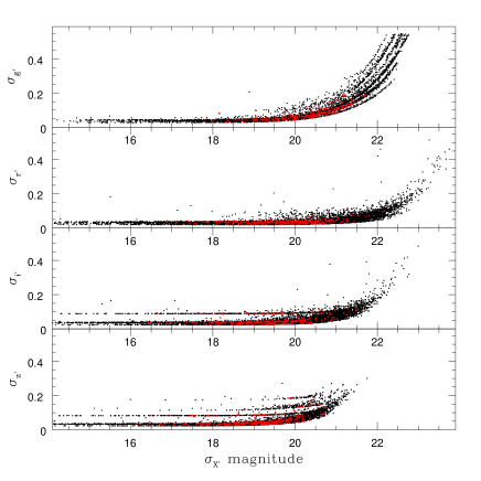
Figure 1.— From top to bottom, photometric uncertainties as a function of magnitude for the $g^{\prime}$, $r^{\prime}$, $i^{\prime}$, and $z^{\prime}$ filters. 7,026 sources measured in the NGC 5128 field are shown, with matched GCs over-plotted in red (visible in the online edition). Sources with systematically larger uncertainties (the thin sequences sitting above the main populations) correspond to objects in regions not overlapped by the pointings, and thus measured once.

Table 1 $g^{\prime}r^{\prime}i^{\prime}z^{\prime}$ Photometry Catalog Of NGC 5128 GCs

ID	$\alpha$	$\delta$	V	$g^{\prime}$	$\sigma_{g^{\prime}}$	$r^{\prime}$	$\sigma_{r^{\prime}}$	$i^{\prime}$	$\sigma_{i^{\prime}}$	$z^{\prime}$	$\sigma_{z^{\prime}}$
	(J2000)	(J2000)
GC001	00:53:40.08	-42:56:51.995	18.75	19.255	0.033	18.477	0.025	18.086	0.034	17.858	0.031
GC039	00:53:38.58	-43:06:26.660	19.45	20.046	0.059	19.129	0.034	18.683	0.038	18.417	0.037
GC043	00:53:38.70	-42:53:35.130	99.00	99.000	99.00	21.718	0.068	21.188	0.091	99.000	99.00
GC045	00:53:38.74	-42:59:48.380	20.23	20.439	0.086	19.891	0.047	19.442	0.048	19.137	0.046
GC046	00:53:38.75	-43:01:45.605	19.22	19.708	0.054	19.017	0.038	18.722	0.042	18.552	0.039
…	…	…	…	…	…	…	…	…	…	…	…

Note. — Table 1 in its entirety can be found in the Appendix.

We used the GC database from Woodley et al. (2007, 2010a, 2010b) to match 605 confirmed GCs in NGC 5128 to our catalog of $g^{\prime}r^{\prime}i^{\prime}z^{\prime}$ measurements. To obtain the most complete set of correlations, we tried matches out to a search radius of $5\hbox{${}^{\prime\prime}$}$, although we found that $\sim 95\%$ of the matches were unique to within $0.8\hbox{${}^{\prime\prime}$}$ with an average angular separation of $0.25\hbox{${}^{\prime\prime}$}$, consistent with the astrometric accuracy described above. Any remaining duplicates that were clearly false matches were eliminated through their very different colors or magnitudes. Our final list contains $g^{\prime}r^{\prime}i^{\prime}z^{\prime}$ photometry for 323 confirmed GCs of NCG 5128, representing $\sim 80\%$ of the known GCs within our field of view. The median uncertainty in the GC photometry for the $g^{\prime}$, $r^{\prime}$, $i^{\prime}$, and $z^{\prime}$ filters is 0.069, 0.035, 0.040, and 0.040, respectively. A truncated version of the catalog is given in Table 1, with the entire listing available in the online edition. The successive columns give the ID number from Woodley et al. (2007, 2010a, 2010b), J2000 coordinates from these studies, the $V$ magnitude from Peng et al. (2004b), and the $g^{\prime}r^{\prime}i^{\prime}z^{\prime}$ magnitudes with their internal uncertainties. Any “99.00” values indicate no data.

3. Color-Magnitude and Two-Color Diagrams

Figure 2 shows the color-magnitude diagrams of all measured objects in our NGC 5128 field in the form $r^{\prime}_{0}$ versus $(g^{\prime}-r^{\prime})_{0}$, $(g^{\prime}-i^{\prime})_{0}$, and $(g^{\prime}-z^{\prime})_{0}$. The GCs are over-plotted in red. The photometry is corrected for foreground reddening with $A_{r}^{\prime}=0.879\cdot A_{V}=0.33$, $E_{g^{\prime}-r^{\prime}}=0.10$, $E_{r^{\prime}-i^{\prime}}=0.07$, $E_{i^{\prime}-z^{\prime}}=0.04$ (Fukugita et al., 1996). As noted above, about 95% of the objects in this diagram are field contamination, with most concentrated along $(g^{\prime}-i^{\prime})_{0}\sim 1$. In Figure 3 we show the color-magnitude diagrams for the GCs only. The characteristic bimodal color distribution is visible in all three plots, although is most obvious in the metallicity-sensitive $(g^{\prime}-i^{\prime})_{0}$ and $(g^{\prime}-z^{\prime})_{0}$ indices.

To estimate the mean colors of each mode, we used the magnitude interval $18<r^{\prime}<20$ to avoid excessive random errors at the faint end and any systematic effects of the mass/metallicity relation at the bright end (see Harris 2009a). We used RMIX to fit bimodal Gaussian distributions, yielding $\langle g^{\prime}-i^{\prime}\rangle_{0}=0.85\pm 0.02$ (blue), $1.13\pm 0.02$ (red), and also $\langle g^{\prime}-z^{\prime}\rangle_{0}=0.98\pm 0.03$ (blue), $1.35\pm 0.04$ (red). The relative fractions of GCs are $0.63\pm 0.07$ in the blue and $0.37\pm 0.07$ in the red. It is worth noting here that Woodley et al. (2010b) found tentative evidence for a trimodal metallicity distribution directly from the spectroscopic line indices for about 70 clusters. The third, intermediate-color mode may be due to a small proportion of somewhat younger clusters (see Woodley et al., 2010b, for additional discussion). We find no clear evidence for a third, intermediate mode in our data, but larger and more precise samples may reveal it. The color histograms from our data, along with the bimodal solution described above, are shown in Figure 4.

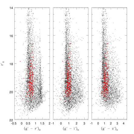
Figure 2.— Color-magnitude diagrams for all measured NGC 5128 sources, with matched GCs over-plotted in red points (visible in the online edition).

Figure 3.— Color-magnitude diagrams of the 323 matched GCs in NGC 5128.

This NGC 5128 data can now be used to investigate the intrinsic colors of GCs in the $g^{\prime}r^{\prime}i^{\prime}z^{\prime}$ indices. As already established in previous photometric and spectroscopic work (e.g. Woodley et al., 2010b; Harris et al., 2004a), the great majority of the GCs in this galaxy follow the classic pattern of large age and bimodal metallicity distribution like other giant ellipticals, so their range in color is already well restricted, with few genuinely young, blue objects. To specify these intrinsic colors a bit further, we look for their distributions in color-color space, relative to the field stars. Figure 5 shows three of the possible six color-color diagrams, again including all measured NGC 5128 sources, with the GCs over-plotted in red. In each graph, we define regions containing $90\%$ of the GC population. Objects outside these boxes have a high probability of being either contaminants or star clusters that are not classically old. The slopes of the boxes shown in Figure 5 are $\Delta(g^{\prime}-r^{\prime})/\Delta(r^{\prime}-i^{\prime})$ = 1.47, $\Delta(g^{\prime}-i^{\prime})/\Delta(g^{\prime}-z^{\prime})$ = 0.79, and $\Delta(r^{\prime}-i^{\prime})/\Delta(i^{\prime}-z^{\prime})$ = 0.74. The regions of higher GC density highlight the intrinsic colors of typical GCs in these colors, showing that the typical GC population is confined to small regions in color-color space and that half of the field objects can be rejected this way. Perhaps the most effective single diagrams are $(g^{\prime}-r^{\prime})$ versus $(r^{\prime}-i^{\prime})$ and $(r^{\prime}-i^{\prime})$ versus $(i^{\prime}-z^{\prime})$ which define the narrowest zones.

Figure 4.— Upper panel: Histogram of $(g^{\prime}-i^{\prime})_{0}$ colors for our sample of GCs in NGC 5128. The dashed lines give the bimodal deconvolution for the color distribution described in the text, while the solid line is the sum of both components. Lower panel: Histogram of $(g^{\prime}-z^{\prime})_{0}$ colors for the same clusters. As above, the dashed lines give the bimodal solution for the color distribution, while the solid line is the total for the bimodal fit.

8

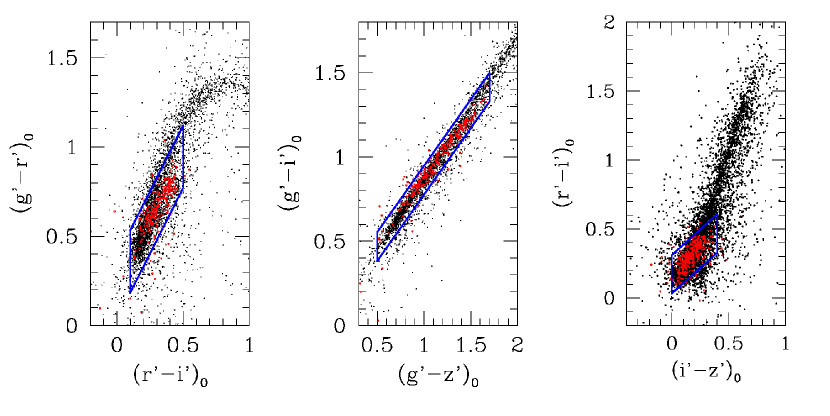
Figure 5.— Color-color diagrams for the NGC 5128 field objects, with the known GCs over-plotted in red. The blue boxes highlight regions encapsulating $90\%$ of the GCs in each of the three color-color planes.

4. Calibration versus Metallicity

As mentioned above, one of the goals of our study was to define the baseline conversion of the $g^{\prime}r^{\prime}i^{\prime}z^{\prime}$ color indices to metallicity, for “typical” old GCs. Ideally, transformation of a given color index to (say) [Fe/H] would be done by having in hand both the photometric indices and the [Fe/H] values as determined by high-dispersion spectroscopy. Peng et al. (2006) present a preliminary calibration of this type for $(g-z)$ versus [Fe/H], using their unpublished photometry for 40 Milky Way clusters, plus 55 more from the Virgo giants M87 and M49 (see their Figs. 11 and 12), along with a variety of literature sources for the spectroscopy.

In our case, high-dispersion and high-signal-to-noise ($S/N$) spectroscopy for the clusters in NGC 5128 are as yet available for only a small number of objects (see, e.g. Rejkuba et al., 2007; Taylor et al., 2010). However, Woodley et al. (2010b) present a recent spectroscopic study of a large sample of the NGC 5128 and Milky Way GCs through the use of Lick indices. A significant advantage of their database is that it analyzes the line indices of clusters within both galaxies on an internally homogeneous and self-consistent system, allowing a more reliable comparison. We use the material from their study here, realizing that it may be superseded once a more extensive database of high-dispersion spectroscopic metallicities becomes available.

Here we work with the two most metallicity-sensitive color indices ($g^{\prime}-i^{\prime}$, $g^{\prime}-z^{\prime}$) and derive their transformations into [Fe/H] in two steps. The first of these is their correlation against the Lick index [MgFe]^′, defined as

$${\rm[MgFe]}^{\prime}\,=\,\sqrt{Mg_{b}\times(0.72Fe5270\,+\,0.28Fe5335)}$$

(Thomas et al., 2003). [MgFe]^′ is designed to be a relatively clean heavy-element abundance indicator, highly insensitive to [$\alpha$/Fe] variations. In Figure 6, we show the dereddened color indices versus this index for the NGC 5128 clusters in our catalog that are in common with Woodley et al. (2010b). We find in both cases that linear relations match the data well, given by

$$\begin{split}\@add@centering\centering(g^{\prime}-i^{\prime})_{0}=&(0.575\pm 0.039)+(0.203\pm 0.021){\rm[MgFe]}^{\prime}\\ &(n=61)\end{split}$$ (5)

$$\begin{split}\@add@centering\centering(g^{\prime}-z^{\prime})_{0}=&(0.660\pm 0.048)+(0.253\pm 0.025){\rm[MgFe]}^{\prime}\\ &(n=59).\end{split}$$ (6)

In both cases the rms scatter around these mean lines is $\pm 0.13$ mag in color.

Figure 6.— Correlation of intrinsic color indices $(g^{\prime}-i^{\prime})_{0}$ and $(g^{\prime}-z^{\prime})_{0}$ against the Lick metallicity index [MgFe]^′ for the GCs in NGC 5128, with spectroscopic data from Woodley et al. (2010b).

The second step is to transform [MgFe]^′ to metallicity, [Fe/H]. Here we use the Milky Way GCs, which have metallicity measurements superior to those of any other galaxy. We adopt [Fe/H] values from the catalog of Harris (1996) (2003 edition) and correlate these against their [MgFe]^′ values measured in Woodley et al. (2010b) from Milky Way GC spectra obtained from Puzia et al. (2002) and Schiavon et al. (2005). The results for 40 Milky Way clusters are shown in Figure 7. We note here that the catalog values of [Fe/H] were originally based on the Zinn & West (1984) scale. However, a large number of abundance measurements from high-dispersion spectroscopy have been added, making the current Milky Way catalog list of metallicities close to the Carretta & Gratton (1997) scale.

An interesting question raised by Figure 7 is whether or not the conversion is adequately matched by a linear relation. From Puzia et al. (2002), Woodley et al. (2010b), and Harris (1996), we estimate that the typical uncertainty in each quantity is $\pm 0.1$ dex. We find the best-fit linear or quadratic relations to be

$$\centering{\rm[MgFe]}^{\prime}=(2.987\pm 0.075)+(1.347\pm 0.062){\rm[Fe/H]}\hskip 8.5359pt{\rm(linear)}\@add@centering$$ (7)

$$\begin{split}\@add@centering\centering{\rm[MgFe]}^{\prime}=&(3.253\pm 0.120)+(1.966\pm 0.230){\rm[Fe/H]}\\ &+(0.281\pm 0.104){\rm[Fe/H]}^{2}\hskip 8.5359pt{\rm(quadratic)}.\end{split}$$ (8)

The rms scatter around these relations is $\pm 0.19$ (linear) and $\pm 0.17$ (quadratic). Given also that the solution for the [Fe/H]² term is significant at the $3\sigma$ level, we therefore find a slight preference for the quadratic solution and recommend it for future use. We note that Peng et al. (2006) also found that a single linear transformation for $(g-z)$ to [Fe/H] was not suitable. Fig. 7 shows, however, that in the range $-1.7\lesssim$ [Fe/H] $\lesssim-0.3$ that contains the great majority of clusters, the difference between the linear and quadratic conversions is small.

Figure 7.— Correlation of the Lick metallicity index [MgFe]^′ against heavy-element abundance [Fe/H] for GCs in the Milky Way. The dashed and solid lines show the linear and quadratic best-fit solutions given in the text. A typical error bar is shown as a cross in the upper left corner.

Combining the two steps outlined above, our color to metallicity conversions are

$$\centering(g^{\prime}-i^{\prime})_{0}=1.235+0.399{\rm[Fe/H]}+0.057{\rm[Fe/H]}^{2},\@add@centering$$ (9)

$$\centering(g^{\prime}-z^{\prime})_{0}=1.483+0.497{\rm[Fe/H]}+0.071{\rm[Fe/H]}^{2},\@add@centering$$ (10)

At a mean typical GC metallicity [Fe/H] $\simeq-1$, we therefore have $\Delta(g^{\prime}-i^{\prime})/\Delta[Fe/H]\simeq 0.29$ and $\Delta(g^{\prime}-z^{\prime})/\Delta[Fe/H]\simeq 0.36$. With good photometric measurement precisions of $\pm 0.05$, the $g^{\prime}i^{\prime}z^{\prime}$ indices can then be used to predict metallicities to within internal uncertainties of typically $\pm 0.15$ dex.

We can compare our recommended conversion of $(g^{\prime}-z^{\prime})_{0}$ to [Fe/H] with that of Peng et al. (2006); both curves are shown in Figure 8. For this purpose, the very small differences between the $gz$ and $g^{\prime}z^{\prime}$ systems mentioned earlier are unimportant. Peng et al. adopt a two-section linear curve with the changeover point at [Fe/H] $\sim-1$, roughly halfway between the normal metal-poor and metal-rich GC sequences, and compare their data with several population-synthesis models (see their Figure 12). The internal scatter of their [Fe/H] data points around their adopted calibration is not specifically listed but appears to be $\pm 0.2-0.3$ dex. The differences between their curve and the one we have derived here are within $\sim 0.1$ dex over most of the range. While the Milky Way GCs constrain our transformation in the range -2.0 $\lesssim$ [Fe/H] $\lesssim$ -0.5 (0.7 $\lesssim$ $(g^{\prime}-z^{\prime})_{0}$ $\lesssim$ 1.3), we note our transformation agrees well with Peng et al. for [Fe/H] $\gtrsim$ -0.5. Close inspection of the data used by Peng et al. (see their Fig. 12) indicates that our continuous quadratic transformation falls close to the centroid of their data, and fits the calibration as well as any of the various model curves shown there.

The conversions derived above can be used to determine the mean metallicities of the NGC 5128 GCs. If we adopt the mean colors obtained in Section 3, we find [Fe/H] = $-1.19$ (blue), $-0.27$ (red) from a direct average of $(g^{\prime}-i^{\prime})_{0}$ and $(g^{\prime}-z^{\prime})_{0}$. The two colors give the same metallicities to within $\pm 0.05$ dex. In addition, the Peng et al. (2006) calibration for $(g-z)$ gives the same means to within $\pm 0.04$ dex. These values are $\simeq 0.1$ dex more metal-rich than has often been obtained in other giant ellipticals (e.g. Geisler et al., 1996; Brodie & Strader, 2006; Harris, 2009a), but they fall within the expected range given the combined internal uncertainties in the photometric calibration, reddenings, and transformation coefficients.

Another consistency check of the external accuracy of these transformations can be done by comparing our results with the $gri$ photometry of the M87 cluster system by Harris (2009b). The data from that study consist of photometry for several thousand GCs throughout the M87 halo, placed accurately on the SDSS standard system by reference to the SDSS-DR5 catalog of sources in the same region. The blue and red GC sequences in M87 are located at mean intrinsic colors $\langle g-i\rangle_{0}$(blue) = 0.80, $\langle g-i\rangle_{0}$(red) = 1.07, obtained using $E_{g-i}=0.03$. These translate through the preceding equations into mean metallicities of [Fe/H] = $-1.47$ (blue), $-0.56$ (red), which are both within $\pm 0.1$ dex of the metallicities for the two sequences in giant galaxies obtained through a variety of other methods (e.g. Brodie & Strader, 2006).

Figure 8.— Comparison of our calibration of $(g^{\prime}-z^{\prime})_{0}$ versus metallicity (solid line) with the Peng et al. (2006) calibration (dashed line). While the Peng et al. (2006) calibration is carried out on the F475W and F850W ($g$ and $z$) Advanced Camera for Surveys (ACS) filters, we plot their transformation here as $(g^{\prime}-z^{\prime})_{0}$ since the differences between the filter systems are negligible for the purposes of this comparison.

5. Comparison of Filter Systems

As noted in the Introduction, broadband photometry with a metallicity-sensitive color index is a fast and effective way to derive first-order MDFs for GC systems, though ultimately not as accurate (or internally precise) as spectroscopic indices. Many different color indices have been used in published studies for this purpose, and it is of interest to gauge how the $u^{\prime}g^{\prime}r^{\prime}i^{\prime}z^{\prime}$ filter system compares with others. The well known Johnson/Cousins $(V-I)$ is not an especially sensitive index (see Barmby et al., 2000), but it was adopted particularly in many early HST-based studies that were crucial to defining the bimodality paradigm (e.g. Gebhardt & Kissler-Patig, 1999; Larsen et al., 2001, among many others) essentially because the heavily used Wide Field Planetary Camera 2 (WFPC2) camera had relatively low blue response. Two other common indices are $(B-I)$ (e.g. Harris, 2009a) and $(C-T_{1})$ (e.g. Geisler et al., 1996; Harris et al., 2004b). For comparison, the equations linking them to [Fe/H] are

$$(V-I)_{0}\,=\,1.15+0.156{\rm[Fe/H]}$$ (11)

$$(B-I)_{0}\,=\,2.158+0.375{\rm[Fe/H]}$$ (12)

$$(C-T_{1})_{0}\,=\,1.998+0.748{\rm[Fe/H]}+0.138{\rm[Fe/H]}^{2}$$ (13)

trim whitespace on eps Their slopes near the mid-range [Fe/H] $\simeq-1$ are 0.156 for $(V-I)$, 0.37 for $(B-I)$, and 0.47 for $(C-T_{1})$, compared to 0.285 for $(g^{\prime}-i^{\prime})$ and 0.355 for $(g^{\prime}-z^{\prime})$. Of these five, the Washington index $(C-T_{1})_{0}$ appears to be the most sensitive to metallicity because of its wide baseline and also because the $C$ filter is positioned directly over a large number of heavy-element absorption lines. A more complete comparison of the Johnson/Cousins color indices, including the various pairs that can be constructed from $UBVRIJK$, is given by Barmby et al. (2000).

The use of the near-UV filter in the $u^{\prime}g^{\prime}r^{\prime}i^{\prime}z^{\prime}$ system could in principle yield an even more sensitive index such as $(u^{\prime}-i^{\prime})$ or $(u^{\prime}-z^{\prime})$, but (for most ground-based cameras) at a huge penalty in exposure time. Combinations of optical filters with near-infrared filters have also been explored, such as the combination of $B$ and $R$ with the 3.6$\mu$ color (Spitler et al., 2008), or $(V-K)$ (Barmby et al., 2000). These have a very wide baseline and can “split” the bimodal GC sequences more clearly, but have the disadvantage that the observations require two sets of instrumentation.

We regard both $(g^{\prime}-i^{\prime})_{0}$ and $(g^{\prime}-z^{\prime})_{0}$ as competitive color indices for GC MDF photometry, though both $(B-I)_{0}$ and $(C-T_{1})_{0}$ continue to be effective for this purpose as well. These four indices all provide good compromises between intrinsic metallicity sensitivity and the necessary exposure times to obtain precise photometry. For ground-based photometry, an extra factor to consider is the degree of fringing present in the red or near-infrared filters. For example, the fringing was fairly large in the $z^{\prime}$ filter in this work (as noted above) and this may reduce the internal precision that can be achieved for $(g^{\prime}-z^{\prime})$, offsetting the advantage of its wider color baseline.

Figure 9.— Color distribution in the Washington index $(C-T_{1})_{0}$ for 500 clusters in NGC 5128. The bimodal fit to the data is shown in the dashed lines for the blue and red modes, with the sum in the solid line.

The data in the Woodley et al. (2010a) catalog also provide a convenient summary of the $(C-T_{1})$ color indices extracted from the Washington-system survey of the NGC 5128 field (Harris et al., 2004a). The color distribution for 500 clusters in the magnitude range $17<T_{1}<21$ is shown in Figure 9. Earlier versions of the $(C-T_{1})$ distribution based on much smaller numbers of individually selected clusters were derived in Harris et al. (1992); Woodley et al. (2005, 2010b). A bimodal-Gaussian fit to this distribution yields mean colors for the two modes of $1.413\pm 0.038$ (blue), $1.902\pm 0.038$ (red), with proportions $0.565\pm 0.074$ (blue), $0.435\pm 0.074$ (red). There is no significant presence of additional modes.

6. Conclusions

In this study we have used new ground-based photometry to generate a database of $g^{\prime}r^{\prime}i^{\prime}z^{\prime}$ indices for the GCs in NGC 5128, the nearest giant elliptical galaxy. Our data have been calibrated against fundamental USNO standard stars and thus provide among the first comprehensive calibrations of intrinsic GC colors in the $g^{\prime}r^{\prime}i^{\prime}z^{\prime}$ system. Our final data list contains colors and magnitudes for 323 known GCs covering the metallicity range $-2<$ [Fe/H] $<0$.

Adding this material to previously published high-S/N spectroscopic indices for clusters in NGC 5128 and the Milky Way, we derive transformations between $(g^{\prime}-i^{\prime})_{0},(g^{\prime}-z^{\prime})_{0}$, [MgFe]^′, and [Fe/H]. These transformations can be used to determine metallicity distributions from the USNO color indices to a typical precision of $\pm 0.15$ dex. Comparison with other widely used photometric indices indicates that the colors constructed from $g^{\prime}i^{\prime}z^{\prime}$ are competitive with other broadband optical indices such as $(B-I)$ or $(C-T_{1})$.

$g^{\prime}r^{\prime}i^{\prime}z^{\prime}$ Photometry Catalog Of NGC 5128 GCs GC001	00:53:40.08	-42:56:51.995	18.75	19.255	0.033	18.477	0.025	18.086	0.034	17.858	0.031
GC039	00:53:38.58	-43:06:26.660	19.45	20.046	0.059	19.129	0.034	18.683	0.038	18.417	0.037
GC043	00:53:38.70	-42:53:35.130	99.00	99.000	99.00	21.718	0.068	21.188	0.091	99.000	99.00
GC045	00:53:38.74	-42:59:48.380	20.23	20.439	0.086	19.891	0.047	19.442	0.048	19.137	0.046
GC046	00:53:38.75	-43:01:45.605	19.22	19.708	0.054	19.017	0.038	18.722	0.042	18.552	0.039
GC047	00:53:38.90	-43:08:43.215	18.80	19.184	0.044	18.538	0.033	18.298	0.038	18.166	0.036
GC048	00:53:38.91	-42:53:07.105	19.85	20.433	0.068	19.577	0.025	19.068	0.035	18.734	0.032
GC049	00:53:38.91	-42:58:16.350	19.51	19.966	0.056	19.276	0.034	18.935	0.038	18.765	0.038
GC052	00:53:39.02	-42:59:33.490	19.30	19.553	0.048	19.087	0.034	18.894	0.038	18.830	0.038
GC053	00:53:39.05	-43:02:24.460	19.89	20.531	0.076	19.606	0.035	19.116	0.040	18.785	0.039
GC054	00:53:39.10	-43:04:11.555	19.16	19.687	0.054	99.000	0.037	18.677	0.041	18.528	0.042
GC055	00:53:39.11	-43:01:18.385	18.95	19.459	0.049	18.758	0.036	18.431	0.040	18.275	0.039
GC056	00:53:39.14	-43:06:01.640	18.91	19.581	0.050	18.605	0.035	18.097	0.038	17.756	0.037
GC057	00:53:39.16	-42:58:29.825	19.10	19.591	0.048	18.850	0.034	18.501	0.038	18.325	0.034
GC058	00:53:39.16	-42:57:51.130	19.73	20.289	0.066	19.429	0.034	18.951	0.038	18.649	0.038
GC060	00:53:39.20	-43:08:14.200	18.49	19.058	0.046	18.229	0.038	17.856	0.041	17.675	0.040
GC061	00:53:39.25	-42:52:35.325	99.00	20.431	0.069	19.733	0.027	19.353	0.037	19.213	0.042
GC062	00:53:39.26	-42:57:48.435	19.05	19.555	0.050	18.853	0.036	18.515	0.040	18.328	0.038
GC063	00:53:39.29	-43:08:17.650	20.34	20.845	0.096	20.134	0.038	19.788	0.043	19.550	0.052
GC064	00:53:39.34	-43:07:36.160	20.44	20.818	0.094	20.366	0.037	20.050	0.043	19.820	0.055
GC066	00:53:39.39	-43:01:22.860	18.86	19.466	0.049	18.580	0.036	18.135	0.039	17.872	0.038
GC068	00:53:39.47	-43:04:32.645	20.08	99.000	0.065	19.384	0.047	19.119	0.053	19.026	0.072
GC070	00:53:39.55	-43:04:34.690	19.20	19.702	0.051	18.965	0.035	18.637	0.038	18.490	0.039
GC071	00:53:39.60	-43:04:24.460	19.92	20.369	0.068	19.669	0.035	19.388	0.038	19.268	0.044
GC072	00:53:39.61	-42:54:50.440	19.25	19.714	0.041	19.051	0.028	18.735	0.035	18.568	0.034
GC073	00:53:39.62	-43:03:15.415	19.84	20.265	0.067	19.692	0.036	19.350	0.040	19.250	0.042
GC074	00:53:39.62	-42:53:24.568	17.25	17.807	0.033	16.936	0.026	16.497	0.035	16.235	0.032
GC075	00:53:39.63	-43:05:34.615	19.96	20.553	0.078	19.645	0.034	19.180	0.039	18.835	0.039
GC076	00:53:39.64	-42:48:59.070	19.44	19.926	0.068	19.181	0.039	18.847	0.091	18.719	0.084
GC077	00:53:39.65	-43:01:21.680	17.91	18.556	0.043	17.640	0.039	17.187	0.042	16.914	0.040
GC079	00:53:39.70	-43:09:58.330	99.00	99.000	99.00	22.132	0.097	21.480	0.108	99.000	99.00
GC082	00:53:39.74	-42:54:29.540	99.00	20.412	0.055	19.529	0.026	19.026	0.035	18.705	0.032
GC083	00:53:39.74	-43:10:16.430	20.45	20.946	0.146	20.251	0.044	20.144	0.052	20.196	0.070
GC085	00:53:39.81	-43:08:42.590	99.00	99.000	99.00	21.041	0.058	20.492	0.058	20.102	0.071
GC086	00:53:39.83	-43:01:08.095	18.38	18.963	0.042	18.057	0.034	17.594	0.038	17.293	0.035
GC087	00:53:39.83	-42:59:23.305	18.74	19.250	0.046	18.545	0.035	18.221	0.038	18.031	0.036
GC088	00:53:39.84	-43:05:32.685	20.02	20.657	0.087	19.814	0.041	19.313	0.046	19.059	0.051
GC089	00:53:39.85	-42:55:48.370	99.00	21.028	0.107	20.841	0.040	20.911	0.064	99.000	99.00
GC090	00:53:39.86	-42:52:04.920	99.00	99.000	99.00	21.787	0.071	21.249	0.082	99.000	99.00
GC091	00:53:39.88	-42:56:10.305	17.71	18.314	0.032	17.439	0.028	16.989	0.037	16.714	0.035
GC095	00:53:39.99	-43:09:08.480	99.00	21.202	0.183	20.474	0.038	20.216	0.048	20.009	0.058
GC096	00:53:40.01	-42:54:08.835	20.43	20.953	0.080	20.146	0.027	19.735	0.037	19.502	0.044
GC098	00:53:40.04	-43:05:30.190	19.74	20.314	0.068	19.475	0.035	19.048	0.039	18.813	0.036
GC102	00:53:40.10	-43:08:32.910	99.00	99.000	99.00	21.290	0.050	20.732	0.060	99.000	99.00
GC103	00:53:40.11	-42:54:40.783	19.37	19.602	0.039	19.362	0.028	19.201	0.037	19.083	0.037
GC104	00:53:40.11	-42:50:51.150	99.00	99.000	99.00	21.093	0.031	20.646	0.052	20.619	0.089
GC106	00:53:40.12	-43:09:25.375	18.04	18.507	0.042	17.767	0.037	17.482	0.040	17.323	0.039
GC107	00:53:40.12	-42:52:27.597	99.00	20.774	0.087	20.075	0.026	19.747	0.038	19.550	0.041
GC109	00:53:40.21	-42:56:25.345	18.93	19.482	0.037	18.630	0.026	18.193	0.035	17.909	0.032
GC110	00:53:40.21	-43:03:02.415	18.68	19.231	0.044	18.387	0.034	17.954	0.038	17.685	0.035
GC111	00:53:40.22	-42:57:40.555	19.73	20.186	0.062	19.466	0.034	19.115	0.038	18.891	0.040
GC113	00:53:40.22	-42:50:45.932	18.44	19.036	0.037	18.105	0.026	17.604	0.035	17.291	0.033
GC115	00:53:40.25	-42:51:21.545	99.00	21.158	0.118	20.473	0.028	20.237	0.042	20.080	0.081
GC116	00:53:40.28	-43:00:19.630	19.34	19.744	0.050	19.053	0.033	18.846	0.038	18.632	0.035
GC118	00:53:40.31	-43:07:21.705	19.61	20.044	0.059	19.380	0.033	19.103	0.038	18.964	0.037
GC119	00:53:40.32	-43:09:38.790	18.60	19.064	0.044	18.305	0.035	18.009	0.039	17.827	0.036
GC120	00:53:40.33	-42:57:15.285	17.41	17.967	0.038	17.115	0.034	16.694	0.038	16.427	0.034
GC121	00:53:40.35	-42:58:05.780	19.62	20.182	0.062	19.340	0.034	18.934	0.038	18.685	0.039
GC126	00:53:40.49	-43:08:29.535	20.78	99.000	99.00	20.563	0.041	20.207	0.055	20.017	0.080
GC127	00:53:40.49	-43:06:20.455	20.04	20.580	0.078	19.833	0.035	19.471	0.042	19.273	0.045
GC129	00:53:40.51	-43:01:15.190	18.12	18.708	0.041	17.815	0.034	17.363	0.038	17.062	0.035
GC130	00:53:40.57	-43:02:57.155	18.91	19.553	0.051	18.679	0.043	18.215	0.041	17.925	0.041
GC131	00:53:40.59	-43:09:09.475	19.42	19.882	0.075	19.181	0.035	18.879	0.040	18.732	0.039
GC132	00:53:40.59	-43:04:14.795	19.29	19.902	0.055	19.048	0.035	18.632	0.039	18.320	0.036
GC135	00:53:40.63	-42:55:18.493	19.12	19.560	0.037	18.898	0.026	18.579	0.035	18.411	0.032
GC136	00:53:40.68	-43:02:06.670	19.71	20.374	0.069	19.356	0.033	18.876	0.038	18.531	0.035
GC137	00:53:40.68	-42:55:09.492	19.46	19.972	0.043	19.119	0.025	18.655	0.035	18.321	0.033
GC138	00:53:40.68	-42:53:32.802	17.80	18.405	0.031	17.556	0.026	17.102	0.035	16.837	0.033
GC140	00:53:40.70	-43:03:23.870	20.40	99.000	0.107	20.162	0.038	19.731	0.045	19.407	0.054
GC141	00:53:40.74	-43:01:31.905	99.00	20.441	0.072	19.522	0.035	19.031	0.039	18.704	0.037
GC142	00:53:40.74	-42:58:03.165	18.92	19.309	0.043	18.682	0.032	18.442	0.037	18.315	0.034
GC143	00:53:40.74	-43:03:09.470	19.51	99.000	0.057	19.343	0.035	18.982	0.040	18.821	0.037
GC144	00:53:40.80	-43:04:19.145	19.78	20.403	0.070	19.535	0.035	19.116	0.039	18.847	0.039
GC145	00:53:40.81	-42:57:25.280	18.62	19.162	0.045	18.372	0.035	18.002	0.038	17.811	0.037
GC147	00:53:40.82	-42:58:07.690	20.44	20.983	0.104	20.188	0.035	19.818	0.043	19.587	0.050
GC149	00:53:40.86	-42:57:00.157	19.57	20.019	0.046	19.367	0.026	19.035	0.035	18.869	0.037
GC150	00:53:40.86	-43:07:59.020	18.20	18.725	0.040	17.888	0.033	17.520	0.038	17.286	0.034
GC152	00:53:40.88	-43:02:31.230	99.00	99.000	99.00	21.189	0.052	20.803	0.070	99.000	99.00
GC153	00:53:40.89	-42:52:12.122	19.82	20.562	0.074	19.725	0.036	19.276	0.047	19.013	0.049
GC154	00:53:40.92	-43:07:32.380	20.70	21.223	0.189	20.417	0.037	20.033	0.045	19.686	0.052
GC155	00:53:40.93	-42:57:42.635	18.72	19.036	0.041	18.514	0.032	18.285	0.037	18.170	0.033
GC158	00:53:40.95	-43:07:23.395	19.55	20.177	0.063	19.281	0.037	18.799	0.040	18.523	0.039
GC160	00:53:41.01	-42:50:30.400	19.87	20.395	0.086	19.676	0.040	19.409	0.091	19.293	0.086
GC161	00:53:41.01	-42:57:45.665	20.25	20.696	0.085	20.053	0.035	19.764	0.043	19.620	0.047
GC162	00:53:41.02	-43:08:39.105	20.78	99.000	99.00	20.477	0.036	20.112	0.045	19.774	0.052
GC164	00:53:41.06	-43:06:03.140	20.39	20.957	0.101	20.154	0.038	19.765	0.042	19.564	0.047
GC165	00:53:41.07	-43:05:06.320	19.59	20.103	0.062	19.371	0.036	19.031	0.041	18.807	0.039
GC170	00:53:41.10	-43:03:32.985	20.44	21.051	0.113	20.128	0.035	19.802	0.043	19.648	0.048
GC173	00:53:41.13	-43:03:07.880	99.00	20.921	0.151	20.336	0.038	99.000	0.049	19.881	0.061
GC174	00:53:41.13	-43:09:27.900	19.43	19.858	0.073	19.160	0.035	18.833	0.040	18.651	0.040
GC180	00:53:41.22	-42:53:04.598	19.07	19.607	0.039	18.839	0.026	18.467	0.035	18.261	0.034
GC181	00:53:41.23	-43:04:09.685	20.11	20.570	0.078	19.880	0.035	19.531	0.043	19.318	0.046
GC185	00:53:41.32	-42:58:27.280	20.50	21.155	0.185	20.372	0.048	19.933	0.054	19.746	0.066
GC186	00:53:41.33	-43:07:43.690	20.11	20.844	0.151	20.077	0.043	19.629	0.043	19.363	0.051
GC187	00:53:41.36	-42:54:08.297	20.47	20.891	0.077	20.243	0.027	19.950	0.039	19.792	0.049
GC188	00:53:41.38	-43:06:35.725	20.44	21.021	0.159	20.133	0.036	19.736	0.042	19.539	0.048
GC194	00:53:41.56	-42:53:26.012	20.00	20.537	0.061	19.779	0.027	19.421	0.038	19.199	0.039
GC195	00:53:41.63	-43:07:58.987	19.47	19.962	0.043	19.188	0.022	18.853	0.025	18.675	0.027
GC196	00:53:41.69	-42:58:21.465	20.26	20.859	0.096	20.099	0.036	19.650	0.042	19.435	0.044
GC196	00:53:41.70	-42:58:17.850	20.26	20.762	0.109	20.042	0.043	19.606	0.048	19.415	0.053
GC197	00:53:41.70	-42:56:31.335	20.06	20.465	0.072	19.849	0.026	19.481	0.037	19.255	0.039
GC199	00:53:41.72	-43:05:16.615	19.88	20.345	0.055	19.684	0.023	19.376	0.027	19.208	0.033
GC200	00:53:41.73	-43:03:25.670	19.10	19.312	0.033	18.833	0.023	18.670	0.026	18.582	0.028
GC203	00:53:41.79	-42:52:39.748	19.81	20.225	0.050	19.574	0.026	19.254	0.035	19.070	0.040
GC204	00:53:41.79	-43:09:40.585	19.53	19.965	0.044	19.291	0.023	99.000	0.027	18.889	0.028
GC205	00:53:41.87	-43:04:02.140	19.18	19.758	0.043	18.915	0.023	18.450	0.026	18.141	0.027
GC207	00:53:41.92	-43:04:21.652	99.00	18.748	0.030	18.067	0.021	17.822	0.025	17.710	0.024
GC208	00:53:41.95	-42:57:47.290	18.57	19.007	0.041	18.298	0.032	17.974	0.037	18.014	0.024
GC208	00:53:41.96	-42:57:42.680	18.57	19.003	0.051	18.314	0.036	99.000	0.040	17.749	0.035
GC209	00:53:41.96	-42:53:25.420	20.46	20.885	0.078	20.203	0.027	19.916	0.039	19.837	0.048
GC210	00:53:41.96	-42:58:09.840	19.49	20.059	0.057	19.148	0.033	18.667	0.038	18.327	0.035
GC210	00:53:41.97	-42:58:05.970	19.49	19.874	0.069	19.164	0.036	18.700	0.040	18.289	0.036
GC211	00:53:41.97	-42:54:44.325	19.26	19.818	0.041	18.940	0.026	18.492	0.035	18.209	0.033
GC214	00:53:41.99	-43:05:09.253	99.00	21.031	0.102	20.287	0.025	19.890	0.030	19.758	0.038
GC215	00:53:42.01	-42:56:47.095	18.36	99.000	99.00	18.063	0.039	17.681	0.090	17.464	0.083
GC219	00:53:42.04	-43:03:47.225	99.00	20.971	0.110	20.242	0.037	20.200	0.060	19.905	0.068
GC224	00:53:42.11	-42:58:04.330	19.97	20.304	0.088	19.699	0.039	19.208	0.044	18.718	0.040
GC226	00:53:42.11	-42:55:15.380	20.08	99.000	99.00	19.941	0.042	19.739	0.093	19.614	0.091
GC228	00:53:42.12	-43:05:45.805	99.00	20.511	0.162	20.345	0.066	20.102	0.056	99.000	99.00
GC229	00:53:42.16	-43:07:17.137	20.15	20.634	0.077	19.948	0.024	19.669	0.028	19.497	0.033
GC230	00:53:42.17	-42:58:46.630	18.86	19.372	0.053	18.504	0.036	18.094	0.040	17.779	0.035
GC231	00:53:42.19	-42:56:24.365	18.64	99.000	99.00	18.425	0.040	18.169	0.091	18.024	0.083
GC232	00:53:42.19	-43:07:02.545	18.77	19.299	0.044	18.501	0.030	18.129	0.033	17.955	0.037
GC233	00:53:42.19	-43:04:29.102	19.37	19.943	0.043	19.036	0.022	18.590	0.025	18.293	0.025
GC234	00:53:42.22	-42:59:00.200	20.35	99.000	99.00	20.053	0.040	19.591	0.047	19.222	0.050
GC235	00:53:42.25	-43:02:49.360	99.00	20.928	0.105	19.965	0.037	19.359	0.047	19.059	0.046
GC236	00:53:42.26	-43:03:51.313	99.00	21.133	0.110	20.219	0.024	19.730	0.030	19.390	0.035
GC238	00:53:42.28	-42:58:57.560	19.10	19.500	0.061	18.787	0.036	18.392	0.040	18.135	0.035
GC239	00:53:42.28	-42:56:59.205	19.03	99.000	99.00	18.976	0.050	18.804	0.098	18.626	0.091
GC245	00:53:42.34	-42:56:45.320	18.68	99.000	99.00	18.499	0.041	18.258	0.091	18.114	0.084
GC246	00:53:42.34	-42:53:00.645	20.25	20.826	0.116	99.000	0.040	19.493	0.091	19.182	0.085
GC248	00:53:42.35	-43:05:29.037	99.00	18.158	0.081	18.167	0.030	17.809	0.030	17.632	0.032
GC250	00:53:42.37	-43:08:37.300	20.80	21.366	0.162	20.612	0.046	20.240	0.054	20.038	0.075
GC251	00:53:42.39	-43:07:27.980	20.92	20.633	0.104	20.623	0.026	20.142	0.032	19.876	0.041
GC252	00:53:42.40	-42:53:39.920	20.17	20.655	0.107	19.913	0.041	19.551	0.092	19.358	0.087
GC253	00:53:42.43	-43:08:04.000	99.00	99.000	99.00	21.526	0.074	21.277	0.120	99.000	99.00
GC255	00:53:42.50	-43:05:44.950	19.64	20.028	0.064	19.307	0.022	18.863	0.025	18.559	0.026
GC258	00:53:42.56	-43:05:02.597	99.00	18.832	0.040	17.899	0.021	17.575	0.025	17.408	0.024
GC259	00:53:42.56	-43:03:28.615	99.00	19.837	0.053	19.219	0.028	18.924	0.031	18.754	0.031
GC261	00:53:42.58	-43:05:34.612	99.00	20.634	0.113	20.284	0.030	19.936	0.035	19.811	0.040
GC262	00:53:42.61	-43:04:33.762	99.00	21.029	0.088	20.205	0.023	19.742	0.029	19.488	0.045
GC264	00:53:42.64	-43:04:01.340	19.96	20.542	0.062	19.738	0.025	19.301	0.028	19.045	0.032
GC265	00:53:42.65	-42:55:59.015	17.63	99.000	99.00	17.394	0.041	17.100	0.091	16.949	0.084
GC266	00:53:42.66	-43:05:01.785	17.53	18.024	0.038	17.277	0.023	16.941	0.026	16.756	0.027
GC267	00:53:42.66	-43:03:09.430	99.00	20.280	0.120	20.437	0.075	20.101	0.075	19.569	0.077
GC268	00:53:42.70	-42:56:00.970	20.34	99.000	99.00	20.320	0.041	19.955	0.094	19.678	0.090
GC271	00:53:42.72	-43:05:00.220	99.00	99.000	99.00	21.030	0.048	20.926	0.067	20.723	0.130
GC272	00:53:42.73	-43:08:16.042	19.84	20.256	0.062	19.619	0.023	19.381	0.027	19.226	0.031
GC273	00:53:42.77	-42:58:04.870	19.99	20.573	0.089	19.694	0.038	19.323	0.043	19.109	0.042
GC274	00:53:42.78	-43:03:45.695	99.00	21.147	0.145	20.681	0.030	20.287	0.037	20.005	0.046
GC275	00:53:42.80	-43:10:41.750	19.26	19.791	0.055	19.107	0.033	18.874	0.035	18.609	0.043
GC276	00:53:42.81	-43:03:19.275	99.00	20.527	0.063	19.837	0.024	19.487	0.028	19.310	0.032
GC277	00:53:42.82	-42:59:13.970	18.39	18.829	0.050	18.108	0.036	17.790	0.040	17.598	0.035
GC278	00:53:42.84	-42:58:59.370	18.81	19.283	0.054	18.530	0.036	18.151	0.040	17.917	0.036
GC279	00:53:42.83	-43:03:41.380	20.39	20.978	0.084	20.065	0.024	19.701	0.029	19.486	0.036
GC281	00:53:42.89	-42:58:33.750	19.42	19.954	0.066	19.127	0.036	18.686	0.040	18.394	0.036
GC283	00:53:42.90	-43:04:56.412	99.00	19.336	0.046	18.495	0.023	18.084	0.026	17.852	0.027
GC284	00:53:42.92	-43:07:54.975	19.83	20.251	0.063	19.651	0.023	19.406	0.027	19.298	0.031
GC286	00:53:42.96	-42:58:56.140	18.58	19.061	0.052	18.304	0.036	17.949	0.040	17.705	0.035
GC286	00:53:42.94	-42:59:00.410	18.58	19.039	0.068	18.281	0.047	17.962	0.061	17.579	0.174
GC289	00:53:43.07	-42:57:15.630	18.37	18.782	0.050	18.175	0.037	17.910	0.041	17.730	0.036
GC289	00:53:43.06	-42:57:20.505	18.37	99.000	99.00	18.194	0.041	17.983	0.091	17.871	0.084
GC290	00:53:43.06	-43:06:45.435	99.00	21.275	0.128	20.593	0.027	20.222	0.033	20.072	0.046
GC291	00:53:43.07	-42:56:53.175	19.63	99.000	99.00	19.415	0.040	19.178	0.091	19.037	0.085
GC295	00:53:43.11	-42:57:03.115	19.87	99.000	99.00	19.565	0.039	19.145	0.090	18.933	0.084
GC296	00:53:43.11	-42:53:48.230	20.05	99.000	99.00	19.804	0.041	19.459	0.091	19.222	0.087
GC297	00:53:43.13	-43:08:06.673	19.23	19.741	0.049	18.940	0.022	18.581	0.025	18.399	0.026
GC299	00:53:43.14	-43:06:08.877	19.92	20.429	0.069	19.670	0.023	19.308	0.027	19.168	0.030
GC300	00:53:43.19	-43:00:42.485	19.71	20.183	0.060	19.525	0.029	19.192	0.035	19.047	0.045
GC305	00:53:43.29	-43:02:20.205	19.55	20.023	0.046	19.306	0.023	18.964	0.025	18.756	0.027
GC307	00:53:43.31	-43:05:04.680	20.12	20.740	0.085	19.830	0.023	19.368	0.027	19.077	0.030
GC311	00:53:43.35	-43:06:08.560	20.17	20.729	0.083	19.926	0.023	19.520	0.027	19.250	0.031
GC312	00:53:43.36	-43:04:08.225	19.97	20.470	0.073	19.713	0.023	19.336	0.027	19.151	0.031
GC313	00:53:43.36	-43:00:30.650	20.42	20.892	0.113	20.321	0.044	20.070	0.053	20.052	0.072
GC314	00:53:43.37	-42:57:58.020	19.42	19.926	0.062	19.209	0.036	18.969	0.041	18.840	0.040
GC315	00:53:43.40	-42:55:36.140	99.00	99.000	99.00	20.562	0.045	20.281	0.095	20.150	0.134
GC316	00:53:43.43	-42:59:26.500	19.92	20.393	0.081	19.692	0.040	19.367	0.046	19.168	0.048
GC317	00:53:43.44	-42:59:44.240	19.82	20.286	0.075	19.617	0.038	19.307	0.044	19.105	0.045
GC319	00:53:43.49	-42:58:26.260	19.62	20.107	0.069	19.364	0.036	19.073	0.043	18.834	0.041
GC320	00:53:43.52	-43:05:46.455	17.87	18.364	0.039	17.614	0.023	17.276	0.026	17.086	0.026
GC321	00:53:43.53	-42:58:37.970	19.97	20.477	0.084	19.670	0.038	19.284	0.043	19.021	0.044
GC322	00:53:43.53	-43:01:59.790	19.00	19.613	0.048	18.630	0.022	18.154	0.025	17.881	0.024
GC325	00:53:43.57	-43:03:56.548	19.48	20.030	0.055	19.228	0.023	18.817	0.026	18.631	0.027
GC326	00:53:43.58	-42:59:04.270	18.15	18.646	0.047	17.877	0.036	17.537	0.039	17.342	0.034
GC328	00:53:43.62	-42:56:20.570	20.38	99.000	99.00	20.122	0.043	19.899	0.094	19.727	0.091
GC330	00:53:43.65	-42:59:22.330	17.22	17.797	0.045	16.885	0.035	16.431	0.039	16.135	0.034
GC331	00:53:43.68	-42:59:10.670	18.88	19.272	0.063	18.536	0.043	18.095	0.044	17.845	0.040
GC333	00:53:43.75	-43:01:32.508	20.24	20.599	0.074	20.028	0.022	19.857	0.028	19.726	0.038
GC339	00:53:43.90	-43:08:06.315	19.30	19.855	0.051	19.002	0.023	18.583	0.026	18.295	0.025
GC340	00:53:43.91	-43:07:11.070	19.21	19.676	0.049	99.000	0.023	18.692	0.027	18.549	0.028
GC341	00:53:43.93	-42:53:18.925	19.58	99.000	99.00	19.316	0.039	19.018	0.091	18.775	0.116
GC342	00:53:43.97	-42:55:30.730	19.81	99.000	99.00	19.546	0.040	19.349	0.091	19.205	0.085
GC347	00:53:44.05	-43:09:40.055	20.09	20.615	0.090	19.785	0.025	19.413	0.030	19.189	0.030
GC350	00:53:44.07	-43:06:55.325	20.05	99.000	99.00	19.840	0.035	19.559	0.042	19.353	0.045
GC354	00:53:44.15	-43:08:55.683	19.84	20.353	0.067	19.561	0.023	19.187	0.027	18.952	0.029
GC355	00:53:44.17	-43:00:09.260	20.28	20.698	0.099	20.076	0.038	19.823	0.049	19.709	0.055
GC357	00:53:44.19	-42:56:57.320	18.49	99.000	99.00	18.176	0.041	17.794	0.091	17.486	0.084
GC358	00:53:44.19	-43:05:42.973	20.36	20.936	0.096	20.101	0.024	19.675	0.029	19.369	0.032
GC361	00:53:44.28	-42:55:44.770	19.10	99.000	99.00	18.848	0.039	18.605	0.090	18.452	0.083
GC362	00:53:44.31	-43:09:10.233	20.12	20.523	0.070	19.898	0.023	19.658	0.028	19.551	0.035
GC365	00:53:44.36	-42:56:32.630	17.17	99.000	99.00	16.891	0.042	16.642	0.092	16.477	0.084
GC366	00:53:44.42	-42:56:44.400	21.28	99.000	99.00	20.866	0.045	20.422	0.095	20.192	0.132
GC367	00:53:44.43	-43:00:37.578	19.43	19.850	0.051	19.201	0.022	18.932	0.026	18.783	0.028
GC368	00:53:44.44	-43:06:14.542	19.95	20.490	0.069	19.671	0.024	19.284	0.027	19.061	0.031
GC371	00:53:44.46	-43:07:52.703	20.40	20.925	0.095	20.131	0.024	19.780	0.029	19.589	0.034
GC373	00:53:44.57	-42:59:15.520	20.09	20.578	0.093	19.851	0.038	19.526	0.045	19.252	0.045
GC374	00:53:44.59	-43:01:20.995	18.99	19.444	0.044	18.776	0.023	18.490	0.026	18.330	0.027
GC375	00:53:44.64	-43:07:06.085	20.08	20.670	0.082	19.849	0.025	19.438	0.030	19.191	0.033
GC377	00:53:44.66	-42:56:36.385	99.00	99.000	99.00	21.282	0.051	20.963	0.109	20.644	0.150
GC378	00:53:44.71	-42:53:42.970	18.43	99.000	99.00	18.112	0.039	17.800	0.090	17.563	0.083
GC379	00:53:44.86	-43:09:09.253	18.66	19.182	0.042	18.359	0.022	17.955	0.025	17.718	0.026
GC380	00:53:44.95	-43:08:30.492	19.17	19.600	0.046	18.911	0.022	18.636	0.026	18.469	0.026
GC383	00:53:45.15	-43:06:39.352	20.09	20.523	0.072	19.892	0.024	19.587	0.029	19.429	0.035
GC384	00:53:45.31	-43:03:18.465	18.74	19.218	0.044	18.485	0.023	18.122	0.026	17.898	0.026
GC385	00:53:45.35	-43:10:35.350	18.95	19.297	0.043	18.694	0.030	18.449	0.035	18.278	0.038
GC386	00:53:45.37	-43:03:18.398	19.33	19.691	0.067	19.045	0.022	18.635	0.025	18.385	0.026
GC391	00:53:45.47	-42:53:46.175	19.68	99.000	99.00	19.435	0.039	19.231	0.092	19.133	0.086
GC392	00:53:45.47	-42:54:27.010	19.87	99.000	99.00	19.621	0.040	19.445	0.092	19.270	0.087
GC393	00:53:45.47	-43:09:10.808	19.82	20.245	0.061	19.514	0.023	19.224	0.026	19.054	0.029
GC395	00:53:45.57	-43:03:43.505	19.38	19.841	0.052	19.137	0.030	18.821	0.035	18.612	0.039
GC406	00:53:46.80	-43:07:44.935	17.43	99.000	99.00	17.101	0.027	16.872	0.033	16.718	0.033
GC408	00:53:47.29	-43:04:57.540	20.80	99.000	99.00	20.393	0.042	19.810	0.048	19.386	0.051
GC417	00:53:38.83	-42:51:48.878	99.00	20.000	0.051	19.281	0.025	18.925	0.035	18.746	0.034
GC418	00:53:38.98	-43:06:33.230	99.00	21.122	0.123	20.256	0.050	19.759	0.053	19.477	0.059
GC420	00:53:39.73	-43:02:15.805	99.00	20.851	0.096	20.157	0.038	19.800	0.043	19.683	0.048
GC421	00:53:39.97	-43:06:40.780	99.00	99.000	99.00	20.893	0.052	20.514	0.060	20.110	0.068
GC422	00:53:40.22	-43:08:14.245	99.00	20.678	0.086	19.986	0.037	19.707	0.042	19.535	0.043
GC424	00:53:40.46	-43:02:40.125	99.00	20.165	0.061	19.463	0.035	19.133	0.039	18.958	0.040
GC425	00:53:40.64	-43:04:37.820	99.00	21.053	0.115	20.327	0.039	20.018	0.048	19.913	0.060
GC426	00:53:40.95	-43:04:46.530	99.00	20.845	0.094	20.195	0.040	19.907	0.046	19.709	0.055
GC429	00:53:41.53	-43:08:10.253	99.00	19.501	0.038	18.371	0.022	17.949	0.025	17.724	0.024
GC430	00:53:41.63	-42:57:17.115	99.00	99.000	0.057	19.145	0.025	18.654	0.035	18.368	0.032
GC430	00:53:41.64	-42:57:12.100	99.00	20.019	0.067	19.106	0.036	18.684	0.040	18.310	0.036
GC432	00:53:42.27	-43:10:45.520	99.00	99.000	99.00	20.322	0.041	20.206	0.060	19.873	0.070
GC434	00:53:42.52	-42:56:28.050	99.00	99.000	99.00	18.573	0.039	18.181	0.090	17.909	0.083
GC435	00:53:42.57	-42:57:20.320	99.00	99.000	99.00	19.675	0.040	19.302	0.091	19.011	0.085
GC436	00:53:42.79	-42:58:27.990	99.00	19.514	0.055	18.712	0.036	18.291	0.039	18.013	0.035
GC437	00:53:43.02	-42:54:23.570	99.00	99.000	99.00	20.334	0.043	19.925	0.094	19.693	0.089
GC439	00:53:43.13	-42:55:29.620	99.00	99.000	99.00	19.160	0.040	18.816	0.091	18.585	0.084
GC440	00:53:43.36	-42:51:37.810	99.00	19.905	0.060	19.106	0.036	18.859	0.041	18.609	0.040
GC442	00:53:44.62	-42:53:17.920	99.00	99.000	99.00	19.795	0.042	19.573	0.091	19.312	0.125
GC444	00:53:45.38	-42:53:46.655	99.00	99.000	99.00	20.253	0.040	20.087	0.094	20.076	0.132
GC445	00:53:38.70	-43:01:56.695	99.00	21.169	0.120	20.335	0.037	99.000	0.043	19.715	0.051
GC446	00:53:39.36	-43:04:51.005	99.00	20.397	0.070	19.409	0.033	18.921	0.038	18.589	0.036
GC448	00:53:39.58	-42:57:59.055	99.00	21.371	0.141	20.497	0.039	20.030	0.047	19.800	0.062
GC449	00:53:39.60	-43:00:43.600	99.00	20.836	0.095	99.000	0.036	19.524	0.042	19.146	0.042
GC451	00:53:39.70	-42:59:48.505	99.00	20.427	0.071	19.718	0.035	19.364	0.040	19.157	0.043
GC452	00:53:39.85	-42:58:51.640	99.00	21.691	0.190	20.931	0.040	20.502	0.062	20.435	0.096
GC453	00:53:39.91	-42:58:16.590	99.00	19.552	0.048	18.681	0.034	18.238	0.038	17.929	0.036
GC457	00:53:40.46	-42:57:32.200	99.00	20.657	0.083	19.745	0.033	19.307	0.039	19.000	0.038
GC458	00:53:40.51	-42:55:49.650	99.00	21.495	0.125	21.130	0.032	21.021	0.058	99.000	99.00
GC459	00:53:41.18	-42:56:13.925	99.00	99.000	99.00	21.426	0.037	20.967	0.056	20.673	0.094
GC460	00:53:41.36	-43:06:08.840	99.00	21.021	0.160	20.152	0.039	19.684	0.043	19.440	0.048
GC461	00:53:41.60	-43:03:45.198	99.00	21.172	0.110	20.511	0.029	20.154	0.036	20.195	0.056
GC462	00:53:41.73	-43:03:25.670	99.00	19.312	0.033	18.833	0.023	18.670	0.026	18.582	0.028
GC463	00:53:41.82	-42:58:28.880	99.00	20.172	0.062	19.328	0.034	18.850	0.038	18.592	0.038
GC463	00:53:41.83	-42:58:25.380	99.00	20.161	0.074	19.342	0.038	18.890	0.042	18.601	0.037
GC464	00:53:41.83	-42:55:30.118	99.00	99.000	99.00	20.867	0.030	20.522	0.046	20.198	0.059
GC465	00:53:42.01	-43:06:54.745	99.00	99.000	99.00	21.258	0.040	20.889	0.051	20.397	0.166
GC467	00:53:42.07	-42:58:33.510	99.00	20.163	0.074	19.261	0.040	18.837	0.045	18.560	0.044
GC468	00:53:42.08	-42:55:47.625	99.00	99.000	99.00	21.269	0.051	20.968	0.107	20.575	0.149
GC470	00:53:42.21	-42:54:52.920	99.00	99.000	99.00	20.735	0.055	20.161	0.065	99.000	99.00
GC470	00:53:42.21	-42:54:56.965	99.00	99.000	99.00	20.883	0.047	20.677	0.097	99.000	99.00
GC470	00:53:42.19	-42:55:00.365	99.00	99.000	99.00	20.749	0.049	20.332	0.119	19.845	0.094
GC471	00:53:42.81	-42:57:24.355	99.00	99.000	99.00	19.787	0.046	19.651	0.096	19.511	0.094
GC473	00:53:42.87	-43:00:05.150	99.00	99.000	99.00	20.736	0.053	20.341	0.065	20.170	0.083
GC474	00:53:42.99	-42:58:20.550	99.00	20.768	0.108	20.031	0.047	19.792	0.061	19.647	0.061
GC476	00:53:43.15	-42:57:45.120	99.00	20.034	0.064	19.417	0.036	19.105	0.042	18.938	0.042
GC478	00:53:43.29	-42:59:59.790	99.00	19.710	0.059	19.007	0.037	18.697	0.040	18.569	0.040
GC479	00:53:44.01	-42:59:55.490	99.00	21.511	0.191	21.003	0.048	20.840	0.083	99.000	99.00
GC490	00:53:39.16	-43:09:59.860	99.00	21.343	0.138	20.487	0.037	20.068	0.045	19.784	0.057
GC493	00:53:39.86	-43:07:06.255	99.00	21.269	0.131	20.427	0.038	20.062	0.046	19.795	0.059
GC496	00:53:39.99	-42:57:33.220	99.00	20.602	0.079	19.927	0.034	19.609	0.042	19.436	0.046
GC498	00:53:40.09	-43:05:46.335	99.00	21.724	0.191	20.753	0.040	20.248	0.046	19.857	0.145
GC499	00:53:40.12	-43:03:48.025	99.00	21.678	0.183	20.789	0.041	20.326	0.055	20.046	0.064
GC500	00:53:40.24	-43:01:41.413	99.00	99.000	99.00	20.691	0.035	20.372	0.046	20.187	0.073
GC502	00:53:40.45	-43:08:58.230	99.00	99.000	99.00	21.348	0.080	20.867	0.089	99.000	99.00
GC504	00:53:40.60	-43:08:53.535	99.00	20.844	0.098	20.365	0.040	20.176	0.048	20.123	0.079
GC505	00:53:40.85	-43:01:55.775	99.00	20.811	0.096	20.011	0.038	19.632	0.043	19.367	0.042
GC507	00:53:40.87	-42:55:56.373	99.00	20.463	0.057	19.805	0.026	19.487	0.037	19.286	0.037
GC510	00:53:41.18	-42:52:56.040	99.00	99.000	99.00	20.842	0.046	20.583	0.097	20.350	0.140
GC520	00:53:41.81	-42:58:37.990	99.00	21.146	0.124	20.228	0.036	19.734	0.042	19.548	0.052
GC520	00:53:41.82	-42:58:34.650	99.00	21.304	0.169	20.376	0.046	19.803	0.049	19.611	0.057
GC521	00:53:41.92	-42:53:15.757	99.00	20.777	0.070	19.965	0.026	19.489	0.037	19.243	0.038
GC523	00:53:42.21	-43:09:21.647	99.00	21.265	0.124	20.628	0.026	20.395	0.038	20.239	0.050
GC527	00:53:42.64	-42:58:20.410	99.00	20.576	0.094	20.016	0.040	19.776	0.049	19.600	0.054
GC528	00:53:43.22	-42:55:06.610	99.00	99.000	99.00	20.024	0.040	19.665	0.091	19.387	0.087
GC529	00:53:43.40	-43:08:03.098	99.00	99.000	99.00	20.407	0.027	19.847	0.029	19.574	0.036
GC529	00:53:43.37	-43:08:02.985	99.00	21.050	0.106	20.493	0.034	20.193	0.046	20.325	0.081
GC530	00:53:43.50	-43:02:59.957	99.00	21.367	0.139	20.528	0.025	20.196	0.034	19.956	0.041
GC531	00:53:43.65	-43:01:40.450	99.00	99.000	99.00	20.528	0.039	20.019	0.045	19.609	0.051
GC532	00:53:43.65	-42:52:57.160	99.00	99.000	99.00	20.850	0.049	20.466	0.096	20.166	0.134
GC533	00:53:43.67	-43:10:04.720	99.00	20.952	0.097	20.253	0.023	19.924	0.029	19.725	0.039
GC534	00:53:43.69	-42:53:40.220	99.00	99.000	99.00	20.812	0.045	20.566	0.118	20.379	0.142
GC537	00:53:43.75	-43:02:53.020	99.00	99.000	99.00	20.666	0.035	20.159	0.047	19.874	0.185
GC541	00:53:44.09	-43:02:34.620	99.00	21.529	0.156	20.731	0.026	20.349	0.034	20.173	0.048
GC543	00:53:44.57	-43:04:44.977	99.00	21.148	0.111	20.483	0.025	20.169	0.032	20.078	0.046
GC544	00:53:45.15	-43:09:57.920	99.00	99.000	99.00	21.148	0.039	20.728	0.057	20.348	0.063
GC551	00:53:46.03	-43:03:14.890	99.00	21.020	0.115	20.639	0.038	20.311	0.054	19.942	0.188
GC552	00:53:46.51	-43:10:40.580	99.00	99.000	99.00	21.273	0.116	20.627	0.091	19.981	0.110
GC557	00:53:47.39	-43:07:20.545	99.00	21.369	0.134	20.659	0.035	20.361	0.064	20.020	0.060
GC572	00:53:38.49	-43:06:31.340	99.00	21.315	0.134	20.419	0.038	19.956	0.043	19.578	0.132
GC575	00:53:39.19	-43:08:43.525	99.00	20.270	0.066	19.760	0.033	19.560	0.040	19.519	0.047
GC577	00:53:39.65	-43:08:49.170	99.00	19.668	0.049	19.013	0.033	18.833	0.038	18.729	0.036
GC578	00:53:39.69	-42:58:15.050	99.00	21.443	0.148	20.582	0.036	20.127	0.048	19.845	0.061
GC581	00:53:39.91	-42:58:05.550	99.00	99.000	0.111	20.498	0.046	20.154	0.052	99.000	99.00
GC582	00:53:40.08	-43:04:01.475	99.00	21.226	0.125	20.272	0.037	19.813	0.043	19.480	0.048
GC583	00:53:40.15	-42:56:51.933	99.00	21.185	0.098	20.438	0.028	20.117	0.041	19.887	0.051
GC584	00:53:40.60	-43:10:01.895	99.00	20.381	0.096	19.554	0.034	19.180	0.038	18.949	0.038
GC585	00:53:40.94	-43:02:42.580	99.00	20.707	0.088	20.039	0.037	19.706	0.042	19.680	0.049
GC586	00:53:41.10	-43:06:11.895	99.00	21.235	0.128	20.360	0.037	19.893	0.042	19.593	0.051
GC587	00:53:41.34	-43:03:09.875	99.00	20.545	0.081	19.757	0.037	19.315	0.042	19.103	0.040
GC588	00:53:42.01	-42:54:00.555	99.00	20.759	0.116	20.083	0.040	19.778	0.092	19.750	0.093
GC589	00:53:42.55	-42:54:53.450	99.00	99.000	99.00	19.986	0.040	19.492	0.091	19.259	0.086
GC590	00:53:43.13	-42:52:33.985	99.00	20.339	0.088	19.632	0.040	19.342	0.092	19.109	0.086
GC593	00:53:43.47	-42:55:28.130	99.00	99.000	99.00	19.979	0.040	19.700	0.091	19.521	0.088
GC594	00:53:43.67	-43:00:41.210	99.00	20.756	0.071	20.071	0.023	19.783	0.029	19.647	0.037
GC595	00:53:43.85	-43:05:13.243	99.00	20.722	0.107	19.935	0.030	19.501	0.035	19.328	0.038
GC597	00:53:44.44	-43:07:08.203	99.00	21.067	0.110	20.220	0.026	19.805	0.030	19.579	0.037
GC598	00:53:44.64	-43:08:52.450	99.00	20.569	0.077	19.759	0.025	19.344	0.028	19.008	0.031
GC599	00:53:44.70	-43:01:05.470	99.00	20.810	0.087	19.941	0.023	19.499	0.027	19.289	0.032
GC603	00:53:45.41	-43:02:59.222	99.00	19.779	0.097	20.037	0.022	19.675	0.028	19.406	0.034
GC605	00:53:47.60	-43:05:06.025	99.00	99.000	99.00	19.412	0.036	19.067	0.042	18.787	0.045

References

- Barmby et al. (2000) Barmby, P., Huchra, J. P., Brodie, J. P., Forbes, D. A., Schroder, L. L., & Grillmair, C. J. 2000, AJ, 119, 727
- Beasley et al. (2008) Beasley, M. A., Bridges, T. J., Peng, E., Harris, W. E., Harris, G. L. H., Forbes, D. A., & Mackie, G. 2008, MNRAS, 386, 1443
- Brodie & Strader (2006) Brodie, J. P. & Strader, J. 2006, ARA&A, 44, 193
- Carretta & Gratton (1997) Carretta, E. & Gratton, R. G. 1997, A&AS, 121, 95
- Fukugita et al. (1996) Fukugita, M., Ichikawa, T., Gunn, J. E., Doi, M., Shimasaku, K., & Schneider, D. P. 1996, AJ, 111, 1748
- Gebhardt & Kissler-Patig (1999) Gebhardt, K. & Kissler-Patig, M. 1999, AJ, 118, 1526
- Geisler et al. (1996) Geisler, D., Lee, M. G., & Kim, E. 1996, AJ, 111, 1529
- Graham & Phillips (1980) Graham, J. A. & Phillips, M. M. 1980, ApJ, 239, L97
- Harris (2010a) Harris, G. L. H. 2010a, PASA, in press (arXiv:1004.4907)
- Harris et al. (1992) Harris, G. L. H., Geisler, D., Harris, H. C., & Hesser, J. E. 1992, AJ, 104, 613
- Harris et al. (2002) Harris, G. L. H., Geisler, D., Harris, W. E., & Hesser, J. E. 2002, in IAU Symposium, Vol. 207, Extragalactic Star Clusters, ed. D. P. Geisler, E. K. Grebel, & D. Minniti, 309–+
- Harris et al. (2004a) Harris, G. L. H., Geisler, D., Harris, W. E., Schmidt, B. P., Hesser, J. E., Reid, M., Milne, M., Hulme, S. C., & Kidd, T. T. 2004a, AJ, 128, 712
- Harris et al. (2004b) Harris, G. L. H., Harris, W. E., & Geisler, D. 2004b, AJ, 128, 723
- Harris et al. (2010) Harris, G. L. H., Rejkuba, M., & Harris, W. E. 2010, PASA, in press (arXiv:0911.3180)
- Harris (1996) Harris, W. E. 1996, AJ, 112, 1487
- Harris (2009a) —. 2009a, ApJ, 699, 254
- Harris (2009b) —. 2009b, ApJ, 703, 939
- Harris (2010b) —. 2010b, PhilTransRAS, 368, 889
- Harris et al. (2006) Harris, W. E., Harris, G. L. H., Barmby, P., McLaughlin, D. E., & Forbes, D. A. 2006, AJ, 132, 2187
- Hesser et al. (1986) Hesser, J. E., Harris, H. C., & Harris, G. L. H. 1986, ApJ, 303, L51
- Hesser et al. (1984) Hesser, J. E., Harris, H. C., van den Bergh, S., & Harris, G. L. H. 1984, ApJ, 276, 491
- Jordán et al. (2009) Jordán, A., Peng, E. W., Blakeslee, J. P., Côté, P., Eyheramendy, S., Ferrarese, L., Mei, S., Tonry, J. L., & West, M. J. 2009, ApJS, 180, 54
- Lang et al. (2010) Lang, D., Hogg, D. W., Mierle, K., Blanton, M., & Roweis, S. 2010, AJ, 139, 1782
- Larsen et al. (2001) Larsen, S. S., Brodie, J. P., Huchra, J. P., Forbes, D. A., & Grillmair, C. J. 2001, AJ, 121, 2974
- Mink (2002) Mink, D. J. 2002, in Astronomical Society of the Pacific Conference Series, Vol. 281, Astronomical Data Analysis Software and Systems XI, ed. D. A. Bohlender, D. Durand, & T. H. Handley, 169–+
- Mouhcine et al. (2010) Mouhcine, M., Harris, W. E., Ibata, R., & Rejkuba, M. 2010, MNRAS
- Peacock et al. (2010) Peacock, M. B., Maccarone, T. J., Knigge, C., Kundu, A., Waters, C. Z., Zepf, S. E., & Zurek, D. R. 2010, MNRAS, 402, 803
- Peng et al. (2004a) Peng, E. W., Ford, H. C., & Freeman, K. C. 2004a, ApJS, 150, 367
- Peng et al. (2004b) —. 2004b, ApJ, 602, 705
- Peng et al. (2006) Peng, E. W., Jordán, A., Côté, P., Blakeslee, J. P., Ferrarese, L., Mei, S., West, M. J., Merritt, D., Milosavljević, M., & Tonry, J. L. 2006, ApJ, 639, 95
- Puzia et al. (2002) Puzia, T. H., Saglia, R. P., Kissler-Patig, M., Maraston, C., Greggio, L., Renzini, A., & Ortolani, S. 2002, A&A, 395, 45
- Rejkuba et al. (2007) Rejkuba, M., Dubath, P., Minniti, D., & Meylan, G. 2007, A&A, 469, 147
- Schiavon et al. (2005) Schiavon, R. P., Rose, J. A., Courteau, S., & MacArthur, L. A. 2005, ApJS, 160, 163
- Smith et al. (2002) Smith, J. A., Tucker, D. L., Kent, S., Richmond, M. W., Fukugita, M., Ichikawa, T., Ichikawa, S., Jorgensen, A. M., Uomoto, A., Gunn, J. E., Hamabe, M., Watanabe, M., Tolea, A., Henden, A., Annis, J., Pier, J. R., McKay, T. A., Brinkmann, J., Chen, B., Holtzman, J., Shimasaku, K., & York, D. G. 2002, AJ, 123, 2121
- Spitler et al. (2008) Spitler, L. R., Forbes, D. A., & Beasley, M. A. 2008, MNRAS, 389, 1150
- Stetson (1990) Stetson, P. B. 1990, PASP, 102, 932
- Taylor et al. (2010) Taylor, M. A., Puzia, T. H., Harris, G. L., Harris, W. E., Kissler-Patig, M., & Hilker, M. 2010, ApJ, 712, 1191
- Thomas et al. (2003) Thomas, D., Maraston, C., & Bender, R. 2003, MNRAS, 339, 897
- Tucker et al. (2006) Tucker, D. L., Kent, S., Richmond, M. W., Annis, J., Smith, J. A., Allam, S. S., Rodgers, C. T., Stute, J. L., Adelman-McCarthy, J. K., Brinkmann, J., Doi, M., Finkbeiner, D., Fukugita, M., Goldston, J., Greenway, B., Gunn, J. E., Hendry, J. S., Hogg, D. W., Ichikawa, S., Ivezić, Ž., Knapp, G. R., Lampeitl, H., Lee, B. C., Lin, H., McKay, T. A., Merrelli, A., Munn, J. A., Neilsen, Jr., E. H., Newberg, H. J., Richards, G. T., Schlegel, D. J., Stoughton, C., Uomoto, A., & Yanny, B. 2006, Astronomische Nachrichten, 327, 821
- van den Bergh et al. (1981) van den Bergh, S., Hesser, J. E., & Harris, G. L. H. 1981, AJ, 86, 24
- Woodley et al. (2010a) Woodley, K. A., Gómez, M., Harris, W. E., Geisler, D., & Harris, G. L. H. 2010a, AJ, 139, 1871
- Woodley et al. (2007) Woodley, K. A., Harris, W. E., Beasley, M. A., Peng, E. W., Bridges, T. J., Forbes, D. A., & Harris, G. L. H. 2007, AJ, 134, 494
- Woodley et al. (2005) Woodley, K. A., Harris, W. E., & Harris, G. L. H. 2005, AJ, 129, 2654
- Woodley et al. (2010b) Woodley, K. A., Harris, W. E., Puzia, T. H., Gómez, M., Harris, G. L. H., & Geisler, D. 2010b, ApJ, 708, 1335
- Zinn & West (1984) Zinn, R. & West, M. J. 1984, ApJS, 55, 45