Computing the time-continuous Optimal Mass Transport Problem without Lagrangian techniques

Abstract

This work originates from a heart’s images tracking which is to generate an apparent continuous motion, observable through intensity variation from one starting image to an ending one both supposed segmented. Given two images $\rho_{0}$ and $\rho_{1}$, we calculate an evolution process $\rho(t,\cdot)$ which transports $\rho_{0}$ to $\rho_{1}$ by using the optimal extended optical flow. In this paper we propose an algorithm based on a fixed point formulation and a time-space least squares formulation of the mass conservation equation for computing the optimal mass transport problem. The strategy is implemented in a 2D case and numerical results are presented with a first order Lagrange finite element, showing the efficiency of the proposed strategy.

1 Introduction

Modern medical imaging modalities can provide a great amount of information to study the human anatomy and physiological functions in both space and time. In cardiac Magnetic Resonance Imaging (MRI) for example, several slices can be acquired to cover the heart in 3D and at a collection of discrete time samples over the cardiac cycle. From these partial observations, the challenge is to extract the heart’s dynamics from these input spatio-temporal data throughout the cardiac cycle [12], [13].

Image registration consists in estimating a transformation which insures the warping of one reference image onto another target image (supposed to present some similarity). Continuous transformations are privileged, the sequence of transformations during the estimation process is usually not much considered. Most important is the final resulting transformation and not the way one image will be transformed to the other. Here, we consider a reasonable registration process to continuously map the image intensity functions between two images in the context of cardiac motion estimation and modeling.

The aim of this paper is to present, in the context of extended optical flow, an algorithm to compute the optimal time dependent transportation plan without using Lagrangian techniques.

The paper is organized as follows. The introduction is ended, by recalling the optimal extended optical flow model (OEOF) . In section 2, the algorithm we propose is presented. Its convergence is discussed. In section 3 it is proved that solutions obtained with the proposed algorithm are solutions to the optimal extended optical flow, that is to say to the time dependent optimal mass transportation problem. Section 4 deals with numerical results. A 2D cardiac medical image is considered.

1.1 The OEOF method

Let us denote by $\rho$ the intensity function, and by $v$ the velocity of the apparent motion of brightness pattern. An image sequence is considered via the gray-value map $\rho:Q=(0,1)\times\Omega\rightarrow\mathbb{R}$ where $\Omega\subset\mathbb{R}^{d}$ is a bounded regular domain, the support of images, for $d=1,2,3$. If image points move according to the velocity field $v:\,Q\rightarrow\mathbb{R}^{d}$, then gray values $\rho(t,X(t,x))$ are constant along motion trajectories $X(t,x)$. One obtains the optical flow equation:

$$\frac{d}{dt}\rho(t,X(t,x))=\partial_{t}\rho(t,X(t,x))+\left(\,{v}\,|\,{\nabla_{X}\rho(t,X(t,x))}\,\right)_{\mathbb{R}^{d}}=0.$$ (1)

The assumption that the pixel intensity does not change during the movement is in some cases too restrictive. A weakened assumption sometimes called extended optical flow, can replace the intensity preservation by a mass preservation condition which reads:

$$\partial_{t}\rho+\left(\,{v}\,|\,{\nabla_{x}\rho}\,\right)_{\mathbb{R}^{d}}+\mathop{\rm div}\nolimits{(v)}\rho=0.$$ (2)

The previous equations lead to an ill-posed problem for the unknown $(\rho,v)$. Variational formulations or relaxed minimizing problems for computing jointly $(\rho,v)$ have been first proposed in [4] and after by many other authors. Here our concern is somewhat different. Finding $(\rho,v)$ simultaneously is possible by solving the optimal mass transport problem (3)-(4), developed in [5, 6].

Let $\rho_{0}$ and $\rho_{1}$ be the cardiac images between two times arbitrary fixed to zero and one, the mathematical problem reads: find $\rho$ the gray level function defined from $Q$ with values in $[0,1]$ verifying

$$\left\{\begin{array}[]{l}\partial_{t}\rho(t,x)+\mathop{\rm div}\nolimits(v(t,x)\rho(t,x))=0,\,\text{ in }(0,1)\times\Omega\\ \rho(0,x)=\rho_{0}(x);\quad\rho(1,x)=\rho_{1}(x)\\ \end{array}\right.$$ (3)

The velocity function $v$ is determined in order to minimize the functional:

$$\inf_{\rho,v}\int_{0}^{1}\int_{\Omega}\rho(t,x)\|v(t,x)\|^{2}\,dtdx.$$ (4)

Thus we get an image sequence through the gray-value map $\rho$. Let us mention [3], for example, where the optimal mass transportation approach is used in images processing. For general properties of optimal transportation, the reader is referred to the books by C. Villani [14] and L. Ambrosio et al. [2].

2 Algorithm for solving the Optimal Extended Optical Flow

In what follows, let us specify our hypotheses.

• $\Omega$ is a bounded $C^{2,\alpha}$ domain satisfying the exterior sphere condition.

• $\rho_{i}\in C^{1,\alpha}(\overline{\Omega})$ for $i=1,2$, and $\rho_{0}=\rho_{1}\text{ on }\partial\Omega$. Moreover there exist two constants such that $0<\underline{\beta}\leq\rho_{i}\leq\overline{\beta}$ in $\Omega$.

Let $\rho^{0}\in C^{1,\alpha}([0,1]\times\overline{\Omega})$ be given by $\rho^{0}(t,x)=(1-t)\rho_{0}(x)+t\rho_{1}(x)$. We have $\|\partial_{t}\rho^{0}\|_{C^{0,\alpha}([0,1]\times\overline{\Omega})}\leq C(\rho_{0},\rho_{1})$ and $\partial_{t}\rho^{0}|_{\partial\Omega}=0$.

For each $t\in[0,1]$, our need for problem (3)-(4) is a velocity field vanishing on $\partial\Omega$. To do so, the following method is used.

• Compute

  $$\left\{\begin{array}[]{l}-\mathop{\rm div}\nolimits(\rho^{n}(t,\cdot)\nabla\eta)=0\,\text{ in }\Omega\\ \rho^{n}(t,\cdot)\partial_{n}\eta=1\quad\text{ on }\partial\Omega,\end{array}\right.$$ (5)

  and set $C^{n}(t)=\frac{1}{|\partial\Omega|}\int_{\Omega}\partial_{t}\rho^{n}\eta\,dx$.

• For each $t\in[0,1]$ compute $\varphi^{n+1}$ solution to

  $$\left\{\begin{array}[]{l}-\mathop{\rm div}\nolimits(\rho^{n}(t,\cdot)\nabla\varphi^{n+1})=\partial_{t}\rho^{n}(t,\cdot),\,\text{ in }\Omega\\ \varphi^{n+1}=C^{n}(t)\quad\text{ on }\partial\Omega.\end{array}\right.$$ (6)

• Set $v^{n+1}=\nabla\varphi^{n+1}$.

• Compute $\rho^{n+1}$, $L^{2}$-least squares solution to

  $$\left\{\begin{array}[]{l}\partial_{t}\rho^{n+1}(t,x)+\mathop{\rm div}\nolimits(v^{n+1}(t,x)\rho^{n+1}(t,x))=0,\,\text{ in }(0,1)\times\Omega\\ \rho^{n+1}(0,x)=\rho_{0}(x);\quad\rho^{n+1}(1,x)=\rho_{1}(x).\\ \end{array}\right.$$ (7)

For each $t\in[0,1]$, since $\rho^{n}(t,\cdot)$, and $\partial_{t}\rho^{n}(t,\cdot)\in C^{0,\alpha}(\overline{\Omega})$, theorem 6.14 p. 107 of [11] applies, and there exists a unique $\varphi^{n+1}(t,\cdot)\in C^{2,\alpha}(\overline{\Omega})$ solution of problem (6). In problem (6) the time is a parameter. As the following regularities with respect to time are verified: $\rho^{n}\in C^{1,\alpha};\,\partial_{t}\rho^{n}\in C^{0,\alpha};\,C^{n}\in C^{0,\alpha}$. The classical $C^{2,\alpha}(\overline{\Omega})$ a priori estimates for solutions to elliptic problems allow us to prove that $\varphi^{n+1}$ is a $C^{0,\alpha}$ function with respect to time. So we have:

$$\|\varphi^{n+1}\|_{C^{0,\alpha}([0,1];C^{2,\alpha}(\overline{\Omega}))}\leq M(\|C^{n}\|_{C^{0,\alpha}([0,1])}+\|\partial_{t}\rho^{n}\|_{C^{0,\alpha}([0,1]\times\overline{\Omega})}).$$

Consider the extension of $\varphi^{n+1}$ by $C^{n}$ outside of the domain $\Omega$; still denoted by $\varphi^{n+1}$. Since the right hand side of equation (6) vanishes on $\partial\Omega$, this extension is regular, and the function $v^{n+1}$ vanish outside $\Omega$ and belongs to $C^{0,\alpha}([0,1];C^{1,\alpha}(\mathbb{R}^{2}))$.

Define the two flows $X^{n+1}_{\pm}(s,t,x)\in C^{1,\alpha}([0,1]\times[0,1]\times\mathbb{R}^{2};\mathbb{R}^{2})$ by

$$\left\{\begin{array}[]{l}\frac{d}{ds}X^{n+1}_{\pm}(s,t,x)=\pm v^{n+1}(s,X^{n+1}_{\pm}(s,t,x))\,\text{ in }(0,1)\\ X^{n+1}_{\pm}(t,t,x)=x.\\ \end{array}\right.$$ (8)

We have the following

Lemma 2.1

The $L^{2}$-least squares solution to problem (7) is given by:

$$\begin{array}[]{c}\rho^{n+1}(t,x)=(1-t)\frac{\rho^{2}_{0}(X^{n+1}_{+}(0,t,x))}{\rho^{n}(t,x)}\\ +t\frac{\rho^{2}_{1}(X^{n+1}_{+}(1,t,x))}{\rho^{n}(t,x)}.\end{array}$$ (9)

Moreover, if $0<\underline{\beta}\leq\rho^{n}\leq\overline{\beta}$ in $[0,1]\times\overline{\Omega}$, then $\rho^{n+1}\in C^{1,\alpha}({\color[rgb]{1,0,0}[0,1]\times\Omega)}$, and verifies the same property.

Proof. We have $X^{n+1}_{-}(1-s,1-t,x)=X^{n+1}_{+}(s,t,x)$ for every $(s,t,x)\in[0,1]\times[0,1]\times\mathbb{R}^{2}$ (see for example [1]).

Let us express equation (7) along the integral curves of equation (8). The $L^{2}$-least squares solution to the ordinary differential equation with initial and final conditions reads

$$\begin{array}[]{c}\rho^{n+1}(s,X^{n+1}_{+}(s,t,x)))=(1-s)e^{-\int_{0}^{s}\mathop{\rm div}\nolimits(v^{n+1}(\tau,X^{n+1}_{+}(\tau,t,x)))\,d\tau}\rho_{0}(X^{n+1}_{+}(0,t,x))\\ +se^{\int_{s}^{1}\mathop{\rm div}\nolimits(v^{n+1}(\tau,X^{n+1}_{+}(\tau,t,x)))\,d\tau}\rho_{1}(X^{n+1}_{+}(1,t,x)).\end{array}$$ (10)

Equation (6) gives the following expression for the divergence

$$\mathop{\rm div}\nolimits(v^{n+1}(s,X^{n+1}_{+}(s,t,x))=\mathop{\rm div}\nolimits(v^{n+1}(s,X^{n+1}_{-}(1-s,1-t,x))\\ =\frac{d}{ds}\ln(\rho^{n}(s,X^{n+1}_{-}(1-s,1-t,x))).$$ (11)

The representation formula (9) is straightforwardly deduced from (6). The regularity of the function $\rho^{n+1}$ is a consequence of the regularity of the flow $X_{+}^{n+1}$. $\square$

Let us now consider the convergence of the algorithm (5)-(7).

Theorem 2.2

There exist $(\rho,\varphi)\in C^{1}([0,1]\times\overline{\Omega})\times C^{0}([0,1];C^{2}(\overline{\Omega}))$, $L^{2}$-least squares solution, respectively solution to

$$\left\{\begin{array}[]{l}\partial_{t}\rho(t,x)+\mathop{\rm div}\nolimits(\nabla\varphi(t,x)\rho(t,x))=0,\;\mathrm{in}\,(0,1)\times\Omega\\ \rho(0,x)=\rho_{0}(x);\quad\rho(1,x)=\rho_{1}(x)\;\mathrm{in}\,\Omega\\ \end{array}\right.$$ (12)

$$\left\{\begin{array}[]{l}-\mathop{\rm div}\nolimits(\rho(t,\cdot)\nabla\varphi)=\partial_{t}\rho(t,\cdot),\;\mathrm{in}\,\Omega\\ \varphi=C(t);\,\nabla\varphi=0\;\mathrm{on}\,\partial\Omega\\ \end{array}\right.$$ (13)

with $C(t)$ defined by:

$$\left\{\begin{array}[]{l}-\mathop{\rm div}\nolimits(\rho(t,\cdot)\nabla\eta)=0\;\mathrm{in}\,\Omega\\ \rho(t,\cdot)\,\partial_{n}\eta=1\;\mathrm{on}\,\partial\Omega\\ C=\frac{1}{|\partial\Omega|}\int_{\Omega}\partial_{t}\rho\,\eta\,dx.\end{array}\right.$$ (14)

Proof. Since $\|v^{0}\|_{C^{0,\alpha}([0,1])}+\|\partial_{t}\rho^{0}\|_{C^{0,\alpha}([0,1]\times\overline{\Omega})}$ is bounded, $\|\varphi^{n+1}\|_{C^{0,\alpha}([0,1];C^{2,\alpha}(\overline{\Omega}))}$ and $\|v^{n+1}\|_{C^{0,\alpha}([0,1];C^{1,\alpha}(\mathbb{R}^{2}))}$ are uniformly bounded in $n$.

From lemma 2.1 there exists a unique $\rho^{n+1}$, the $L^{2}$-least squares solution of (7). Let us give an estimate for $D_{3}X_{+}^{n+1}$. Starting from

$$D_{1}X^{n+1}_{+}(s,t,x))=v^{n+1}(s,X^{n+1}_{+}(s,t,x)),$$

we deduce (see [1])

$$\left\{\begin{array}[]{l}D_{3}D_{1}X^{n+1}_{+}(s,t,x)=D_{2}v^{n+1}(s,X^{n+1}_{+}(s,t,x))D_{3}X^{n+1}_{+}(s,t,x)\\ D_{3}X^{n+1}_{+}(t,t,x)=Id.\\ \end{array}\right.$$ (15)

Since $D_{3}D_{1}X^{n+1}_{+}(s,t,x)=D_{1}D_{3}X^{n+1}_{+}(s,t,x)$ we get

$$D_{3}X^{n+1}_{+}(s,t,x)=e^{-\int_{t}^{s}D_{2}(v^{n+1}(\tau,X^{n+1}_{+}(\tau,t,x)))\,d\tau}Id.$$ (16)

Thus $\|D_{3}v_{+}^{n+1}\|_{C^{0,\alpha}([0,1]^{2}\times\mathbb{R}^{2})}$ is uniformly bounded in $n$.

Since we have [1]:

$$D_{2}X^{n+1}_{+}(s,t,x)=\left(\,{v^{n+1}(s,t,x)}\,|\,{D_{3}X^{n+1}_{+}(s,t,x)}\,\right)$$

we obtain a bound for $\|D_{2}v^{n+1}\|_{C^{0,\alpha}([0,1]^{2}\times\mathbb{R}2)}$ independent of $n$.

From theorem 2.1 we deduce that $\|\rho^{n+1}\|_{C^{1,\alpha}([0,1]\times\overline{\Omega})}$ is uniformly bounded. Since the embeddings

$$C^{0,\alpha}([0,1];C^{2,\alpha}(\overline{\Omega}))\hookrightarrow C^{0}([0,1];C^{2}(\overline{\Omega}))\,\mathrm{and}\,C^{1,\alpha}([0,1]\times\overline{\Omega})\hookrightarrow C^{1}([0,1]\times\overline{\Omega})$$

are relatively compact there is a subsequence of $(\rho^{n},\varphi^{n})$ solution to (5)-(7), still denoted by $(\rho^{n},\varphi^{n})$ converging to $(\rho,\varphi)$ in $C^{1}([0,1]\times\overline{\Omega})\times C^{0}([0,1];C^{2}(\overline{\Omega}))$, and $(\rho,\varphi)$ is the solution of (12)-(14) provided the boundary conditions to be justified. The condition $\nabla\varphi^{n}|_{\partial\Omega}=0$ is valid for the approximations $\varphi^{n}$ (since the functions can be extended by $C^{n}$ outside of $\Omega$). So the convergence in $C^{0}([0,1];C^{2}(\overline{\Omega}))$ yields the condition for the gradient of limit function. For the approximations of function $\rho$, the formula given in Lemma 2.1 combined with the regularity result show that the boundary conditions are exactly satisfied. These conditions are thus valid for the limit function due to the convergence in $C^{1}$. $\square$

We will show in the next section that the above least squares solution $\rho$ is in fact a classical solution.

3 Interpretation of solutions to problem (12)-(14)

In this section it is shown that the solution to problem (12)-(14) is a solution to the time dependent optimal mass transportation problem.

From one hand, remark that $\varphi$ solution to problem (13) satisfies:

$$\varphi-C=\underset{\psi\in L^{2}((0,1);H^{1}_{0}(\Omega))}{\rm Argmin}\frac{1}{4}\int_{0}^{1}\|\partial_{t}\rho+\mathop{\rm div}\nolimits(\rho\nabla\psi)\|_{H^{-1}(\Omega)}^{2}\,dt.$$

Since the functions $(\rho,\varphi)$ are sufficiently regular, we have:

$$\varphi-C=\underset{\psi\in L^{2}((0,1);H^{1}_{0}(\Omega)\cap H^{2}(\Omega))}{\rm Argmin}\frac{1}{4}\int_{0}^{1}\|\partial_{t}\rho+\mathop{\rm div}\nolimits(\rho\nabla\psi)\|_{L^{2}(\Omega)}^{2}\,dt.$$

From an other hand, zero is a bound from below of the functional to be minimized with respect to $(u,\psi)$:

$$\begin{array}[]{l}0=\frac{1}{4}\int_{0}^{1}\|\partial_{t}\rho+\mathop{\rm div}\nolimits(\rho\nabla(\varphi-C))\|_{L^{2}(\Omega)}^{2}\,dt\leq\\ \underset{\begin{array}[]{c}\scriptstyle\{\psi\in L^{2}((0,1);H^{1}(\Omega)),\;u\in L^{2}((0,1);L^{2}(\Omega))\\[-8.53581pt] \scriptstyle\partial_{t}u+\mathop{\rm div}\nolimits(-u\nabla\psi))\in L^{2}((0,1);L^{2}(\Omega))\\[-8.53581pt] \scriptstyle\partial_{t}u+\mathop{\rm div}\nolimits(u\nabla\psi)=0\\[-8.53581pt] \scriptstyle\nabla\psi|_{\partial\Omega}=0\\[-8.53581pt] \scriptstyle\psi|_{\partial\Omega}=C\\[-8.53581pt] \scriptstyle u(0)=\rho_{0};\;u(1)=\rho_{1}\text{ in }\Omega\}\end{array}}{\rm Min}\frac{1}{4}\int_{0}^{1}\|\partial_{t}u+\mathop{\rm div}\nolimits(u\nabla\psi)\|_{L^{2}(\Omega)}^{2}\,dt.\end{array}$$

We deduce that $(\rho,\varphi)$, solution to problem (12)-(14), satisfies

$$(\rho,\varphi)=\underset{\begin{array}[]{c}\scriptstyle\{\psi\in L^{2}((0,1);H^{1}(\Omega)),\;u\in L^{2}((0,1);L^{2}(\Omega))\\[-8.53581pt] \scriptstyle\partial_{t}u+\mathop{\rm div}\nolimits(-u\nabla\psi))\in L^{2}((0,1);L^{2}(\Omega))\\[-8.53581pt] \scriptstyle\partial_{t}u+\mathop{\rm div}\nolimits(u\nabla\psi)=0\\[-8.53581pt] \scriptstyle\nabla\psi|_{\partial\Omega}=0\\[-8.53581pt] \scriptstyle\psi|_{\partial\Omega}=C\\[-8.53581pt] \scriptstyle u(0)=\rho_{0};\;u(1)=\rho_{1}\text{ in }\Omega\}\end{array}}{\rm Argmin}\frac{1}{4}\int_{0}^{1}\|\partial_{t}u+\mathop{\rm div}\nolimits(u\nabla\psi)\|_{L^{2}(\Omega)}^{2}\,dt.$$ (17)

Lemma 3.1

Let $(\rho,\varphi)$ be a solution to problem (12)-(14). Then it satisfies

$$(\rho,\varphi)=\underset{\begin{array}[]{c}\scriptstyle\{\partial_{t}u+\mathop{\rm div}\nolimits(u\nabla\psi)=0;\,\nabla\psi|_{\partial\Omega}=0;\\[-8.53581pt] \scriptstyle\psi|_{\partial\Omega}=C;\,u(0)=\rho_{0};\,u(1)=\rho_{1}\text{ in }\Omega\}\end{array}}{\rm Argmin}\ \int_{0}^{1}\|\mathop{\rm div}\nolimits(u\nabla\psi)\|_{H^{-1}(\Omega)}^{2}\,dt.$$ (18)

Proof. This is a simple consequence of $\partial_{t}\rho=-\mathop{\rm div}\nolimits(\rho\nabla\varphi)$, and of the regularity of $\mathop{\rm div}\nolimits(\rho\nabla\varphi)$ which implies $\|\mathop{\rm div}\nolimits(\rho\nabla\varphi)\|_{L^{2}(\Omega)}=\|\mathop{\rm div}\nolimits(\rho\nabla\varphi)\|_{H^{-1}(\Omega)}$. $\square$

Theorem 3.2

Let $(\rho,\varphi)$ be solution to problem (12)-(14), the existence of which is given in Theorem 2.2, then it satisfies:

$$(\rho,\nabla\varphi)=\underset{\{\partial_{t}u+\mathop{\rm div}\nolimits(uv)=0;\,u(0)=\rho_{0};\,u(1)=\rho_{1}\text{ in }\Omega\}}{\rm Argmin}\int_{0}^{1}\int_{\Omega}u\|v\|^{2}\,dxdt.\\$$ (19)

Proof. Choose $u$ regular verifying $0<\underline{\beta}\leq u\leq\overline{\beta}$, and for all $t\in(0,1)$ solve

$$\inf_{\{v\in L^{2}(\Omega)\,\partial_{t}u+\mathop{\rm div}\nolimits(uv)=0\}}\int_{\Omega}u\|v\|^{2}\,dx.$$ (20)

Let $H=H^{1}_{0}(\Omega)$ be equipped with the following inner product:

$$(\theta,\psi)=\int_{\Omega}u\left(\,{\nabla\theta}\,|\,{\nabla\psi}\,\right)\,dx,$$

which induces a semi-norm which is equivalent to the $H^{1}$-norm. The Riez’s theorem claims that for the linear continuous form

$$\mathcal{L}_{u}(\psi)=<-\mathop{\rm div}\nolimits{(uv)},\psi>_{H;H^{\prime}}=<\partial_{t}u,\psi>_{H;H^{\prime}},$$

there is a unique $\theta\in H$ such that

$$\mathcal{L}_{u}(\psi)=\int_{\Omega}u\left(\,{\nabla\theta}\,|\,{\nabla\psi}\,\right)\,dx,\,\forall\psi\in H.$$

Therefore $v=\nabla\theta$ and problem (20) is reduced to

$$\inf_{\{\psi\in H,\,\partial_{t}u+\mathop{\rm div}\nolimits(u\nabla\psi)=0,\,\psi|_{\partial\Omega}=C\}}\int_{\Omega}u\|\nabla\psi\|^{2}\,dx.$$ (21)

Since

$$\int_{\Omega}u\|\nabla\psi\|^{2}\,dx=\|\mathop{\rm div}\nolimits(u\nabla\psi)\|^{2}_{H^{\prime}},$$

problem (21) reads

$$\inf_{\{\psi\in H,\,\partial_{t}u+\mathop{\rm div}\nolimits(u\nabla\psi)=0,\,\psi|_{\partial\Omega}=C\}}\|\mathop{\rm div}\nolimits(u\nabla\psi)\|^{2}_{H^{\prime}}$$ (22)

or

$$\inf_{\{\psi\in H,\,\partial_{t}u+\mathop{\rm div}\nolimits(u\nabla\psi)=0,\,\psi|_{\partial\Omega}=C\}}\frac{1}{4}\|\partial_{t}u+\mathop{\rm div}\nolimits(u\nabla\psi)\|^{2}_{H^{\prime}}.$$ (23)

Gathering lemma 3.1 with the previous result proves the theorem. $\square$

4 Numerical Approximation of the 2D Optimal Extended Optical Flow

The numerical method is based on a finite element time-space $L^{2}$ least squares formulation (see [7]) of the linear conservation law (7).

Define $\widetilde{v}^{n+1}$ as

$$\widetilde{v}^{n+1}=(1,v^{n+1}_{1},v^{n+1}_{2})^{t}$$

and for a sufficiently regular function $\varphi$ defined on $Q$, set

$$\widetilde{\nabla}\varphi=\left(\frac{\partial{\varphi}}{\partial{t}},\frac{\partial{\varphi}}{\partial{x_{1}}},\frac{\partial{\varphi}}{\partial{x_{2}}}\right)^{t},$$

and

$$\widetilde{\mathop{\rm div}\nolimits}(\widetilde{v}^{n+1}\ \varphi)=\frac{\partial{\varphi}}{\partial{t}}+\sum_{i=1}^{2}\frac{\partial{}}{\partial{x_{i}}}(v^{n+1}_{i}\ \varphi).$$

Let $\{\varphi_{1}\cdot\cdot\cdot\varphi_{N}\}$ be a basis of a space-time finite element subspace

$$V_{h}=\{\varphi,\text{ piecewise regular polynomial functions, with }\varphi(0,\cdot)=\varphi(1,\cdot)=0\},$$

for example, a brick Lagrange finite element of order one ([8]). Let $\Pi_{h}$ be the Lagrange interpolation operator. Let also $W_{h}$ be the finite element subspace of $H^{1}_{0}(\Omega)$, where the basis functions $\{\psi_{1}\cdot\cdot\cdot\psi_{M}\}$ are the traces at $t=0$ of basis functions $\{\varphi_{i}\}_{i=1}^{N}$. An approximation of problem (6) is: for a discrete sequence of time $t$ compute

$$\int_{\Omega}(\rho_{h}^{n}(t,\cdot)\left(\,{\nabla(\varphi_{h}^{n+1}-C^{n}(t))}\,|\,{\nabla\psi_{h}}\,\right)\,dx=\int_{\Omega}\partial_{t}\rho_{h}^{n}(t,\cdot)\psi_{h}\,dx\quad\forall\psi_{h}\in W_{h},$$ (24)

and define $\widetilde{v}^{n+1}=\nabla\varphi_{h}^{n+1}$. The $L^{2}$ least squares formulation of problem (7) is defined in the following way. Consider the functional

$$J(c)=\frac{1}{2}\int_{Q}\left(\widetilde{\mathop{\rm div}\nolimits}(\widetilde{v}^{n+1}\ c)+\partial_{t}\rho^{n}_{h}+\widetilde{\mathop{\rm div}\nolimits}\left[\widetilde{v}^{n+1}\ \Pi_{h}\big{(}(1-t)\rho_{0}+t\rho_{1}\big{)}\right]\right)^{2}\,dx\,dt.$$

This functional is convex and coercive in an appropriate anisotropic Sobolev’s space [7]. The minimizer of $J$ is $\rho^{n+1}_{h}-\Pi_{h}\big{(}(1-t)\rho_{0}+t\rho_{1}\big{)}$ which is the solution to the following problem

$$\int_{Q}\widetilde{\mathop{\rm div}\nolimits}(\widetilde{v}^{n+1}\ \rho^{n+1}_{h})\cdot\widetilde{\mathop{\rm div}\nolimits}(\widetilde{v}^{n+1}\ \psi_{h})\,dx\ dt=\\ \int_{Q}\left(-\partial_{t}\rho_{h}^{n}-\widetilde{\mathop{\rm div}\nolimits}\left(\widetilde{v}^{n+1}\,\Pi_{h}\big{(}(1-t)\rho_{0}+t\rho_{1}\big{)}\right)\right)\cdot\widetilde{\mathop{\rm div}\nolimits}(\widetilde{v}^{n+1}\ \psi_{h})\,dx\ dt$$ (25)

for all $\psi_{h}\in V_{h}$, where

$$\rho_{h}=\sum_{i=1}^{N}\rho_{i}\varphi_{i}(t,x).$$

Thus an approximation of the solution to problem (7) is $\rho^{n+1}_{h}-\Pi_{h}\big{(}(1-t)\rho_{0}+t\rho_{1}\big{)}\in V_{h}$.

The iterative strategy described in Section 2 is used to compute an approximated solution, and to reconstruct the systole to diastole images of a slice of a left ventricle. Ten time steps have been used to compute the solution, and 10000 degrees of freedom for the time-space least squares finite element. The approximated fixed point algorithm converges in about 10 iterations with an accuracy of about $10^{-7}$. In the next figure 1, the initial image and the final image are presented.

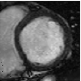
Figure 1: End of diastole of a left ventricular (a), of systole (b)

In the following figure 2, two intermediate times $1/3$ and $2/3$ are shown.

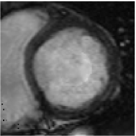
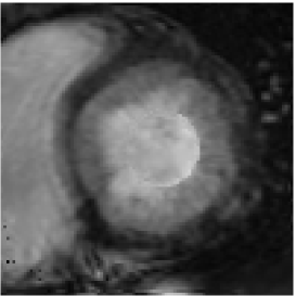
Figure 2: Time step 3 and 6

To summarize, in this work, we present a fixed point algorithm for the computation of the time dependent optimal mass transportation problem, allowing to handle the images tracking problem. The efficiency of the method has been tested with a 2D example.

References

[1] L. Ambrosio, Transport equation and Cauchy problem for BV vector fields.
Invent. math. 158, 227-260, (2004).
[2] L. Ambrosio and N. Gigli and G. Savaré,
Gradient flows in metric spaces and in the space of probability measures.
Lectures in Mathematics ETH Zürich. Birkhäuser Verlag, Basel,
(2008).
[3]
S. Angenent, S. Haker and A. Tannenbaum,
Minimizing Flows for the Monge-Kantorovich Problem, SIAM J. Math. Anal.
35, 61–97, (2003).
[4] G. Aubert, R. Deriche and P. Kornprobst, Computing optical flow
problem via variational techniques. SIAM J. Appl. Math., 80,
156–182, (1999).
[5] J. Benamou and Y. Brenier,
A computational fluid mechanics solution to the Monge-Kantorovich mass transfer problem,
Numer. Math., 84, 375–393, (2000).
[6] J. Benamou,Y. Brenier and K. Guittet, The Monge-Kantorovich mass transfer
and its computational fluid Mechanics formulation.
Int. J. Numer. Math. Fluids 40, 21–30, (2002).
[7] O. Besson and J. Pousin,
Solutions for linear conservation laws with velocity fields in .
Arch. Rational Mech. Anal., 186, 159–175, (2007).
[8] O. Besson and G. de Montmollin,
Space-time integrated least squares: a time marching approach.
Int. J. Numer. Meth. Fluids, 44, 525–543, (2004).
[9]
B. Delhay, P. Clarysse and I.E. Magnin,
Locally adapted
spatio-temporal deformation model for dense motion estimation in
periodic cardiac image sequences,
In Functional Imaging and
Modeling of the Heart, volume LNCS 4466, Salt Lake City, UT, USA,
393–402, (2007).
[10]
B. Delhay, J. Ltjnen, P. Clarysse, T.
Katila, I. E. Magnin, A Dynamic 3-D Cardiac Surface Model
from MR Images. Computers In Cardiology, (2005).
[11] D. Gilbarg, N.S. Trundinger,
Elliptic Partial Differential Equations of
Second Order. Springer, (2001).
[12]
M. Lynch, O. Ghita and P. F. Whelan,
Segmentation of the Left
Ventricle of the Heart in 3D+t MRI Data Using an Optimized Non-Rigid
Temporal Model, IEEE TMI Issue 2, 195–203, (2008).
[13]
J. Schaerer, P. Clarysse, and J. Pousin,
A New Dynamic
Elastic Model for Cardiac Image Analysis.
In Proceedings of the
29th Annual International Conference of the IEEE EMBS, Lyon, France,
4488–4491, (2007).
[14] C. Villani,
Topics in optimal transportation.
Amer. Math. Soc. Providence, Graduate Studies in Mathematics 58, (2003).