Scale dependence of fNLsubscript𝑓𝑁𝐿f_{NL} in N-flation

Qing-Guo Huang 111huangqg@itp.ac.cn
Key Laboratory of Frontiers in Theoretical Physics, Institute of Theoretical Physics, Chinese Academy of Sciences, Beijing 100190, China
Abstract:

Adopting the horizon-crossing approximation, we derive the spectral index of fNLsubscript𝑓𝑁𝐿f_{NL} in general N-flation model. Axion N-flation model is taken as a typical model for generating a large fNLsubscript𝑓𝑁𝐿f_{NL} which characterizes the size of local form bispectrum. We find that its tilt nfNLsubscript𝑛subscript𝑓𝑁𝐿n_{f_{NL}} is negligibly small when all inflatons have the same potential, but a negative detectable nfNLsubscript𝑛subscript𝑓𝑁𝐿n_{f_{NL}} can be achieved in the axion N-flation with different decay constants for different inflatons. The measurement of nfNLsubscript𝑛subscript𝑓𝑁𝐿n_{f_{NL}} can be used to support or falsify the axion N-flation in the near future.

N-flation, non-Gaussianity

1 Introduction

In the single-component slow-roll inflation the different Fourier modes of the curvature perturbation are roughly uncorrelated and their distribution is almost Gaussian [1]. Using δN𝛿𝑁\delta N formalism [2], the curvature perturbation can be expanded to the non-linear orders

ζ=δN=iN,iδϕi+12i,jN,ijδϕiδϕj+16i,j,kN,ijkδϕiδϕjδϕk+,\displaystyle\zeta=\delta N=\sum_{i}N_{,i}\delta\phi_{i}+{1\over 2}\sum_{i,j}N_{,ij}\delta\phi_{i}\delta\phi_{j}+{1\over 6}\sum_{i,j,k}N_{,ijk}\delta\phi_{i}\delta\phi_{j}\delta\phi_{k}+\ ...\ , (1)

where the subscript ,i{,i} denotes the derivative with respect to ϕisubscriptitalic-ϕ𝑖\phi_{i}. The above formula indicates that the curvature perturbation is determined by the evolution of the homogeneous universe corresponding both to the classical inflation trajectory and to nearby trajectories. In principle, an important difference for the multi-field model from the single-component case is that the classical trajectory is not uniquely specified by the potential, but rather has to be given as a separate piece of information. It provides an opportunity to generate a large non-Gaussianity in multi-field slow-roll inflation even at the inflationary epoch [3, 4, 5], not at the end of inflation [6, 7, 8]. See some other relevant references in [9, 10, 11, 12, 13, 14, 15, 17, 16, 18].

On the other hand, not only the size of bispectrum fNLsubscript𝑓𝑁𝐿f_{NL} is measurable, but also its scale dependence characterized by nfNLsubscript𝑛subscript𝑓𝑁𝐿n_{f_{NL}} is possibly measured by the accurate cosmological observations, such as Planck and CMBPol. In [19] the authors concluded that Planck and CMBPol are able to provide a 1-σ𝜎\sigma uncertainty on the spectral index of fNLsubscript𝑓𝑁𝐿f_{NL} for local form bispectrum as follows

ΔnfNL0.150fNL1fskyfor Planck,similar-to-or-equalsΔsubscript𝑛subscript𝑓𝑁𝐿0.150subscript𝑓𝑁𝐿1subscript𝑓𝑠𝑘𝑦for Planck\displaystyle\Delta n_{f_{NL}}\simeq 0.1{50\over f_{NL}}{1\over\sqrt{f_{sky}}}\quad\hbox{for Planck}, (2)

and

ΔnfNL0.0550fNL1fskyfor CMBPol.similar-to-or-equalsΔsubscript𝑛subscript𝑓𝑁𝐿0.0550subscript𝑓𝑁𝐿1subscript𝑓𝑠𝑘𝑦for CMBPol\displaystyle\Delta n_{f_{NL}}\simeq 0.05{50\over f_{NL}}{1\over\sqrt{f_{sky}}}\quad\hbox{for CMBPol}. (3)

Recently the scale dependence of fNLsubscript𝑓𝑁𝐿f_{NL} for inflation and curvaton model is discussed in [20, 21, 22, 23, 24] and a large parameter space for generating a detectable nfNLsubscript𝑛subscript𝑓𝑁𝐿n_{f_{NL}} in curvaton model is illustrated in [22, 23]. The value of nfNLsubscript𝑛subscript𝑓𝑁𝐿n_{f_{NL}} will be an important discriminator to distinguish different models.

In this paper we focus on a class of multi-field inflation, so-called N-flation, in which there are no cross couplings among the inflaton fields or the cross couplings are negligibly small. For an example, we consider the axion N-flation with a detectably large fNLsubscript𝑓𝑁𝐿f_{NL}. But we find that nfNLsubscript𝑛subscript𝑓𝑁𝐿n_{f_{NL}} is negligibly small when all inflatons have the same potential. However, a negative nfNLsubscript𝑛subscript𝑓𝑁𝐿n_{f_{NL}} with detectably large absolute value can be obtained in the model with different decay constants for different inflatons.

Our paper is organized as follows. In Sec. 2 we derive the spectral index of fNLsubscript𝑓𝑁𝐿f_{NL} for general N-flation. We explore the observables, including nfNLsubscript𝑛subscript𝑓𝑁𝐿n_{f_{NL}}, in the axion N-flation in Sec. 3. Some discussions are contained in Sec. 4.

2 Scale dependence of fNLsubscript𝑓𝑁𝐿f_{NL} in general N-flation

In this section we will derive the spectral index of fNLsubscript𝑓𝑁𝐿f_{NL} in general N-flation with Nfsubscript𝑁𝑓N_{f} uncoupled inflaton fields. The potential of inflatons is given by

V=i=1NfVi(ϕi).𝑉superscriptsubscript𝑖1subscript𝑁𝑓subscript𝑉𝑖subscriptitalic-ϕ𝑖\displaystyle V=\sum_{i=1}^{N_{f}}V_{i}(\phi_{i}). (4)

The dynamics of inflation is governed by

H2superscript𝐻2\displaystyle H^{2} =\displaystyle= 13i=1Nf(12ϕ˙i2+Vi(ϕi)),13superscriptsubscript𝑖1subscript𝑁𝑓12superscriptsubscript˙italic-ϕ𝑖2subscript𝑉𝑖subscriptitalic-ϕ𝑖\displaystyle{1\over 3}\sum_{i=1}^{N_{f}}\left({1\over 2}{\dot{\phi}}_{i}^{2}+V_{i}(\phi_{i})\right), (5)
ϕ¨i+3Hϕ˙isubscript¨italic-ϕ𝑖3𝐻subscript˙italic-ϕ𝑖\displaystyle\ddot{\phi}_{i}+3H\dot{\phi}_{i} =\displaystyle= Vi,superscriptsubscript𝑉𝑖\displaystyle-V_{i}^{\prime}, (6)

where Vi=Vi/ϕisuperscriptsubscript𝑉𝑖subscript𝑉𝑖subscriptitalic-ϕ𝑖V_{i}^{\prime}=\partial V_{i}/\partial\phi_{i}. In this paper we work on the unit of Mp=1subscript𝑀𝑝1M_{p}=1. In the slow-roll limit, the above equations are simplified to be

H2superscript𝐻2\displaystyle H^{2} similar-to-or-equals\displaystyle\simeq V3,𝑉3\displaystyle{V\over 3}, (7)
3Hϕ˙i3𝐻subscript˙italic-ϕ𝑖\displaystyle 3H\dot{\phi}_{i} similar-to-or-equals\displaystyle\simeq Vi.superscriptsubscript𝑉𝑖\displaystyle-V_{i}^{\prime}. (8)

Similarly, we introduce some ‘slow-roll’ parameters, such as

ϵi12(ViVi)2.subscriptitalic-ϵ𝑖12superscriptsuperscriptsubscript𝑉𝑖subscript𝑉𝑖2\displaystyle\epsilon_{i}\equiv{1\over 2}\left(V_{i}^{\prime}\over V_{i}\right)^{2}. (9)

From Eq.(7), we find

H˙=16iVi2/V,˙𝐻16subscript𝑖superscriptsubscript𝑉𝑖2𝑉\displaystyle\dot{H}=-{1\over 6}\sum_{i}V_{i}^{\prime 2}/V, (10)

and then

ϵHH˙H2=12iVi2V2,subscriptitalic-ϵ𝐻˙𝐻superscript𝐻212subscript𝑖superscriptsubscript𝑉𝑖2superscript𝑉2\displaystyle\epsilon_{H}\equiv-{\dot{H}\over H^{2}}={1\over 2}{\sum_{i}V_{i}^{\prime 2}\over V^{2}}, (11)

or equivalently,

ϵH=i(ViV)2ϵi.subscriptitalic-ϵ𝐻subscript𝑖superscriptsubscript𝑉𝑖𝑉2subscriptitalic-ϵ𝑖\epsilon_{H}=\sum_{i}({V_{i}\over V})^{2}\epsilon_{i}. (12)

Inflation happens when ϵH<1subscriptitalic-ϵ𝐻1\epsilon_{H}<1. The multi-field slow-roll inflation can be achieved even when some inflaton fields have steep potentials because the friction term for each inflaton is contributed from all of fields.

Following [25], the number of e-folds before the end of inflation is given by

N=i=1NfϕiendϕiViVi𝑑ϕi.𝑁superscriptsubscript𝑖1subscript𝑁𝑓superscriptsubscriptsuperscriptsubscriptitalic-ϕ𝑖𝑒𝑛𝑑subscriptitalic-ϕ𝑖subscript𝑉𝑖superscriptsubscript𝑉𝑖differential-dsubscriptitalic-ϕ𝑖\displaystyle N=\sum_{i=1}^{N_{f}}\int_{\phi_{i}^{end}}^{\phi_{i}}{V_{i}\over V_{i}^{\prime}}d\phi_{i}. (13)

Therefore we obtain

N,i=ViVi,\displaystyle N_{,i}={V_{i}\over V_{i}^{\prime}}, (14)

and

N,ij=(1ViVi′′Vi2)δij.\displaystyle N_{,ij}=\left(1-{V_{i}V_{i}^{\prime\prime}\over V_{i}^{\prime 2}}\right)\delta_{ij}. (15)

Using the δN𝛿𝑁\delta N formalism [2], the power spectrum of scalar perturbation is given by

Pζ=(H2π)2iN,i2.\displaystyle P_{\zeta}=\left({H\over 2\pi}\right)^{2}\sum_{i}N_{,i}^{2}. (16)

A slow-roll inflation model predicts a near scale-invariant power spectrum of scalar perturbation. The deviation from exact scale invariance is described by the spectral index nssubscript𝑛𝑠n_{s} which is defined by

ns1+dlnPζdlnk=12ϵH2i,jϵijN,iN,jkN,k2,\displaystyle n_{s}\equiv 1+{d\ln P_{\zeta}\over d\ln k}=1-2\epsilon_{H}-2{\sum_{i,j}\epsilon_{ij}N_{,i}N_{,j}\over\sum_{k}N_{,k}^{2}}, (17)

where

ϵijViVVjVVi′′Vδij.subscriptitalic-ϵ𝑖𝑗superscriptsubscript𝑉𝑖𝑉superscriptsubscript𝑉𝑗𝑉superscriptsubscript𝑉𝑖′′𝑉subscript𝛿𝑖𝑗\displaystyle\epsilon_{ij}\equiv{V_{i}^{\prime}\over V}{V_{j}^{\prime}\over V}-{V_{i}^{\prime\prime}\over V}\delta_{ij}. (18)

See [25, 26] in detail. In this paper, we assume, without loss of generality, ϕ˙i<0subscript˙italic-ϕ𝑖0\dot{\phi}_{i}<0, so that Vi>0superscriptsubscript𝑉𝑖0V_{i}^{\prime}>0 for ifor-all𝑖\forall\ i. On the other hand, the gravitational wave perturbation is also generated during inflation and the amplitude of its power spectrum is determined by the inflation scale

PT=H2π2/2,subscript𝑃𝑇superscript𝐻2superscript𝜋22\displaystyle P_{T}={H^{2}\over\pi^{2}/2}, (19)

and then the tensor-scalar ratio rTsubscript𝑟𝑇r_{T} becomes

rTPT/Pζ=16/i1ϵi.subscript𝑟𝑇subscript𝑃𝑇subscript𝑃𝜁/16subscript𝑖1subscriptitalic-ϵ𝑖\displaystyle r_{T}\equiv{P_{T}/P_{\zeta}}=16\left/\sum_{i}{1\over\epsilon_{i}}\right.\ . (20)

The amplitude of gravitational perturbation is also near scale-invariant and its tilt is defined by

nTdlnPTdlnk=2ϵH.subscript𝑛𝑇𝑑subscript𝑃𝑇𝑑𝑘2subscriptitalic-ϵ𝐻\displaystyle n_{T}\equiv{d\ln P_{T}\over d\ln k}=-2\epsilon_{H}. (21)

In single-field inflation, rT=16ϵHsubscript𝑟𝑇16subscriptitalic-ϵ𝐻r_{T}=16\epsilon_{H} which leads to a consistency relation nT=rT/8subscript𝑛𝑇subscript𝑟𝑇8n_{T}=-r_{T}/8. For N𝑁N-field inflation, it is modified to be

nTrT/8.subscript𝑛𝑇subscript𝑟𝑇8\displaystyle n_{T}\leq-r_{T}/8. (22)

Here we used the inequality

ϵH1/i1ϵi,subscriptitalic-ϵ𝐻/1subscript𝑖1subscriptitalic-ϵ𝑖\displaystyle\epsilon_{H}\geq 1\left/\sum_{i}{1\over\epsilon_{i}}\right.\ , (23)

where the equality is satisfied when ϵi=ϵHV/Visubscriptitalic-ϵ𝑖subscriptitalic-ϵ𝐻𝑉subscript𝑉𝑖\epsilon_{i}=\epsilon_{H}V/V_{i} for ifor-all𝑖\forall\ i.

From Eq.(1), the non-Gaussianity parameter fNLsubscript𝑓𝑁𝐿f_{NL} can be written by

fNL=56i,jN,iN,jN,ij(kN,k2)2.\displaystyle f_{NL}={5\over 6}\sum_{i,j}{N_{,i}N_{,j}N_{,ij}\over(\sum_{k}N_{,k}^{2})^{2}}. (24)

Since N,ijδijN_{,ij}\propto\delta_{ij} for N-flation, the above formula is simplified to be

fNL=ifNLi,subscript𝑓𝑁𝐿subscript𝑖superscriptsubscript𝑓𝑁𝐿𝑖\displaystyle f_{NL}=\sum_{i}f_{NL}^{i}, (25)

where

fNLi=56N,i2N,ii(kN,k2)2=56rT21281ϵi(1ViVi′′Vi2).\displaystyle f_{NL}^{i}={5\over 6}{N_{,i}^{2}N_{,ii}\over(\sum_{k}N_{,k}^{2})^{2}}={5\over 6}{r_{T}^{2}\over 128}{1\over\epsilon_{i}}\left(1-{V_{i}V_{i}^{\prime\prime}\over V_{i}^{\prime 2}}\right). (26)

Following [21], the spectral index of fNLsubscript𝑓𝑁𝐿f_{NL} for N-flation is

nfNL=1fNLifNLi(2nmulti,i+nf,i),subscript𝑛subscript𝑓𝑁𝐿1subscript𝑓𝑁𝐿subscript𝑖superscriptsubscript𝑓𝑁𝐿𝑖2subscript𝑛𝑚𝑢𝑙𝑡𝑖𝑖subscript𝑛𝑓𝑖\displaystyle n_{f_{NL}}={1\over f_{NL}}\sum_{i}f_{NL}^{i}(2n_{multi,i}+n_{f,i}), (27)

where

nmulti,isubscript𝑛𝑚𝑢𝑙𝑡𝑖𝑖\displaystyle n_{multi,i} =\displaystyle= 2k,lϵkl(N,kN,ljN,j2δilN,kN,i),\displaystyle 2\sum_{k,l}\epsilon_{kl}\left({N_{,k}N_{,l}\over\sum_{j}N_{,j}^{2}}-\delta_{il}{N_{,k}\over N_{,i}}\right), (28)
nf,isubscript𝑛𝑓𝑖\displaystyle n_{f,i} =\displaystyle= kN,kFkii(2)N,ii,\displaystyle-\sum_{k}{N_{,k}F_{kii}^{(2)}\over N_{,ii}}, (29)

and

Fkii(2)=2(ViV)2VkV+Vi′′VVkV+2ViVVi′′VδkiVi′′′Vδki.superscriptsubscript𝐹𝑘𝑖𝑖22superscriptsuperscriptsubscript𝑉𝑖𝑉2superscriptsubscript𝑉𝑘𝑉superscriptsubscript𝑉𝑖′′𝑉superscriptsubscript𝑉𝑘𝑉2superscriptsubscript𝑉𝑖𝑉superscriptsubscript𝑉𝑖′′𝑉subscript𝛿𝑘𝑖superscriptsubscript𝑉𝑖′′′𝑉subscript𝛿𝑘𝑖\displaystyle F_{kii}^{(2)}=-2({V_{i}^{\prime}\over V})^{2}{V_{k}^{\prime}\over V}+{V_{i}^{\prime\prime}\over V}{V_{k}^{\prime}\over V}+2{V_{i}^{\prime}\over V}{V_{i}^{\prime\prime}\over V}\delta_{ki}-{V_{i}^{\prime\prime\prime}\over V}\delta_{ki}. (30)

Considering N,i=Vi/ViN_{,i}=V_{i}/V_{i}^{\prime}, we obtain

nmulti,isubscript𝑛𝑚𝑢𝑙𝑡𝑖𝑖\displaystyle n_{multi,i} =\displaystyle= (1ns2ϵH)4ViVϵi(1ViVi′′Vi2),1subscript𝑛𝑠2subscriptitalic-ϵ𝐻4subscript𝑉𝑖𝑉subscriptitalic-ϵ𝑖1subscript𝑉𝑖superscriptsubscript𝑉𝑖′′superscriptsubscript𝑉𝑖2\displaystyle(1-n_{s}-2\epsilon_{H})-4{V_{i}\over V}\epsilon_{i}\left(1-{V_{i}V_{i}^{\prime\prime}\over V_{i}^{\prime 2}}\right), (31)
nf,isubscript𝑛𝑓𝑖\displaystyle n_{f,i} =\displaystyle= 4(ViV)2ϵiViV(Vi′′ViVi′′′Vi)/(1ViVi′′Vi2).4superscriptsubscript𝑉𝑖𝑉2subscriptitalic-ϵ𝑖/subscript𝑉𝑖𝑉superscriptsubscript𝑉𝑖′′subscript𝑉𝑖superscriptsubscript𝑉𝑖′′′superscriptsubscript𝑉𝑖1subscript𝑉𝑖superscriptsubscript𝑉𝑖′′superscriptsubscript𝑉𝑖2\displaystyle 4({V_{i}\over V})^{2}\epsilon_{i}-{V_{i}\over V}\left({V_{i}^{\prime\prime}\over V_{i}}-{V_{i}^{\prime\prime\prime}\over V_{i}^{\prime}}\right)\left/\left(1-{V_{i}V_{i}^{\prime\prime}\over V_{i}^{\prime 2}}\right)\right.\ . (32)

Using Eqs.(25), (26), (27), (31) and (32), we can easily calculate the spectral index of fNLsubscript𝑓𝑁𝐿f_{NL} in general N-flation. The first term in (31) contribute 2(1ns2ϵH)21subscript𝑛𝑠2subscriptitalic-ϵ𝐻2(1-n_{s}-2\epsilon_{H}) to nfNLsubscript𝑛subscript𝑓𝑁𝐿n_{f_{NL}}. If ϵH1much-less-thansubscriptitalic-ϵ𝐻1\epsilon_{H}\ll 1, 2(1ns2ϵH)0.08similar-to-or-equals21subscript𝑛𝑠2subscriptitalic-ϵ𝐻0.082(1-n_{s}-2\epsilon_{H})\simeq 0.08 for ns=0.96subscript𝑛𝑠0.96n_{s}=0.96.

In addition, we are also interested in the trispectrum in this case. See the Appendix. A in detail.

3 Axion N-flation

In this section we focus on axion N-flation model [5] in which there are Nfsubscript𝑁𝑓N_{f} inflaton fields and the potential of ϕisubscriptitalic-ϕ𝑖\phi_{i} is given by

Vi=Λi4(1cosαi),subscript𝑉𝑖superscriptsubscriptΛ𝑖41subscript𝛼𝑖\displaystyle V_{i}=\Lambda_{i}^{4}(1-\cos\alpha_{i}), (33)

where αi=2πϕi/fisubscript𝛼𝑖2𝜋subscriptitalic-ϕ𝑖subscript𝑓𝑖\alpha_{i}=2\pi\phi_{i}/f_{i} and fisubscript𝑓𝑖f_{i} is the i-th axion decay constant. The ‘slow-roll’ parameters ϵisubscriptitalic-ϵ𝑖\epsilon_{i}’s are given by

ϵi=2π2fi21+cosαi1cosαi,subscriptitalic-ϵ𝑖2superscript𝜋2superscriptsubscript𝑓𝑖21subscript𝛼𝑖1subscript𝛼𝑖\displaystyle\epsilon_{i}={2\pi^{2}\over f_{i}^{2}}{1+\cos\alpha_{i}\over 1-\cos\alpha_{i}}, (34)

and

N,ii=1ViVi′′Vi2=11+cosαi.\displaystyle N_{,ii}=1-{V_{i}V_{i}^{\prime\prime}\over V_{i}^{\prime 2}}={1\over 1+\cos\alpha_{i}}. (35)

Now the number of e-folds before the end of inflation becomes

Ni=1Nf(fi2π)2ln21+cosαi.similar-to-or-equals𝑁superscriptsubscript𝑖1subscript𝑁𝑓superscriptsubscript𝑓𝑖2𝜋221subscript𝛼𝑖\displaystyle N\simeq\sum_{i=1}^{N_{f}}\left({f_{i}\over 2\pi}\right)^{2}\ln{2\over 1+\cos\alpha_{i}}. (36)

Quoting the results in [5], the observables of axion N-flation are

Pζsubscript𝑃𝜁\displaystyle P_{\zeta} =\displaystyle= H28π2i1ϵi,superscript𝐻28superscript𝜋2subscript𝑖1subscriptitalic-ϵ𝑖\displaystyle{H^{2}\over 8\pi^{2}}\sum_{i}{1\over\epsilon_{i}}, (37)
nssubscript𝑛𝑠\displaystyle n_{s} =\displaystyle= 12ϵH8π23H2iΛi4fi21ϵi/j1ϵj,12subscriptitalic-ϵ𝐻8superscript𝜋23superscript𝐻2subscript𝑖/superscriptsubscriptΛ𝑖4superscriptsubscript𝑓𝑖21subscriptitalic-ϵ𝑖subscript𝑗1subscriptitalic-ϵ𝑗\displaystyle 1-2\epsilon_{H}-{8\pi^{2}\over 3H^{2}}\sum_{i}{\Lambda_{i}^{4}\over f_{i}^{2}}{1\over\epsilon_{i}}\left/\sum_{j}{1\over\epsilon_{j}}\right., (38)
rTsubscript𝑟𝑇\displaystyle r_{T} =\displaystyle= 16/i1ϵi,/16subscript𝑖1subscriptitalic-ϵ𝑖\displaystyle 16\left/\sum_{i}{1\over\epsilon_{i}}\right., (39)
fNLsubscript𝑓𝑁𝐿\displaystyle f_{NL} =\displaystyle= 56rT2128i1ϵi11+cosαi.56superscriptsubscript𝑟𝑇2128subscript𝑖1subscriptitalic-ϵ𝑖11subscript𝛼𝑖\displaystyle{5\over 6}{r_{T}^{2}\over 128}\sum_{i}{1\over\epsilon_{i}}{1\over 1+\cos\alpha_{i}}. (40)

Using the results in the previous section, we can calculate the spectral index of fNLsubscript𝑓𝑁𝐿f_{NL} for the axion N-flation, namely

nmulti,isubscript𝑛𝑚𝑢𝑙𝑡𝑖𝑖\displaystyle n_{multi,i} =\displaystyle= (1ns2ϵH)8π23H2Λi4fi2,1subscript𝑛𝑠2subscriptitalic-ϵ𝐻8superscript𝜋23superscript𝐻2superscriptsubscriptΛ𝑖4superscriptsubscript𝑓𝑖2\displaystyle(1-n_{s}-2\epsilon_{H})-{8\pi^{2}\over 3H^{2}}{\Lambda_{i}^{4}\over f_{i}^{2}}, (41)
nf,isubscript𝑛𝑓𝑖\displaystyle n_{f,i} =\displaystyle= 4(ViV)2ϵi2ViVϵi,4superscriptsubscript𝑉𝑖𝑉2subscriptitalic-ϵ𝑖2subscript𝑉𝑖𝑉subscriptitalic-ϵ𝑖\displaystyle 4({V_{i}\over V})^{2}\epsilon_{i}-2{V_{i}\over V}\epsilon_{i}, (42)

and then

nfNLsubscript𝑛subscript𝑓𝑁𝐿\displaystyle n_{f_{NL}} =\displaystyle= 2(1ns2ϵH)16π23H2iΛi4fi21ϵi11+cosαi/j1ϵj11+cosαj21subscript𝑛𝑠2subscriptitalic-ϵ𝐻16superscript𝜋23superscript𝐻2subscript𝑖/superscriptsubscriptΛ𝑖4superscriptsubscript𝑓𝑖21subscriptitalic-ϵ𝑖11subscript𝛼𝑖subscript𝑗1subscriptitalic-ϵ𝑗11subscript𝛼𝑗\displaystyle 2(1-n_{s}-2\epsilon_{H})-{16\pi^{2}\over 3H^{2}}\sum_{i}{\Lambda_{i}^{4}\over f_{i}^{2}}{1\over\epsilon_{i}}{1\over 1+\cos\alpha_{i}}\left/\sum_{j}{1\over\epsilon_{j}}{1\over 1+\cos\alpha_{j}}\right. (43)
+\displaystyle+ 2i(2(ViV)2ViV)11+cosαi/j1ϵj11+cosαj.2subscript𝑖/2superscriptsubscript𝑉𝑖𝑉2subscript𝑉𝑖𝑉11subscript𝛼𝑖subscript𝑗1subscriptitalic-ϵ𝑗11subscript𝛼𝑗\displaystyle 2\sum_{i}\left(2({V_{i}\over V})^{2}-{V_{i}\over V}\right){1\over 1+\cos\alpha_{i}}\left/\sum_{j}{1\over\epsilon_{j}}{1\over 1+\cos\alpha_{j}}\right..

The first and second lines in Eq.(43) are contributed by nmulti,isubscript𝑛𝑚𝑢𝑙𝑡𝑖𝑖n_{multi,i} and nf,isubscript𝑛𝑓𝑖n_{f,i} respectively. Since the second term in nmulti,isubscript𝑛𝑚𝑢𝑙𝑡𝑖𝑖n_{multi,i} is large compared to nf,isubscript𝑛𝑓𝑖n_{f,i} for αiπsimilar-to-or-equalssubscript𝛼𝑖𝜋\alpha_{i}\simeq\pi which corresponds to a large fNLsubscript𝑓𝑁𝐿f_{NL}, the spectral index of fNLsubscript𝑓𝑁𝐿f_{NL} is mainly determined by nmulti,isubscript𝑛𝑚𝑢𝑙𝑡𝑖𝑖n_{multi,i}.

3.1 Axion N-flation with the same potential for different inflatons

In this subsection we discuss the model with Λi=ΛsubscriptΛ𝑖Λ\Lambda_{i}=\Lambda and fi=fsubscript𝑓𝑖𝑓f_{i}=f for ifor-all𝑖\forall\ i in detail. Now the tensor-scalar ratio and fNLsubscript𝑓𝑁𝐿f_{NL} become

rTsubscript𝑟𝑇\displaystyle r_{T} =\displaystyle= 32π2f2/i1cosαi1+cosαi,/32superscript𝜋2superscript𝑓2subscript𝑖1subscript𝛼𝑖1subscript𝛼𝑖\displaystyle{32\pi^{2}\over f^{2}}\left/\sum_{i}{1-\cos\alpha_{i}\over 1+\cos\alpha_{i}}\right., (44)
fNLsubscript𝑓𝑁𝐿\displaystyle f_{NL} =\displaystyle= 10π23f2i1cosαi(1+cosαj)2/(j1cosαj1+cosαj)2,10superscript𝜋23superscript𝑓2subscript𝑖/1subscript𝛼𝑖superscript1subscript𝛼𝑗2superscriptsubscript𝑗1subscript𝛼𝑗1subscript𝛼𝑗2\displaystyle{10\pi^{2}\over 3f^{2}}\sum_{i}{1-\cos\alpha_{i}\over(1+\cos\alpha_{j})^{2}}\left/\left(\sum_{j}{1-\cos\alpha_{j}\over 1+\cos\alpha_{j}}\right)^{2}\right., (45)

and the spectral indices of scalar power spectrum and fNLsubscript𝑓𝑁𝐿f_{NL} are simplified to be

nssubscript𝑛𝑠\displaystyle n_{s} =\displaystyle= 12ϵH8π2Λ43H2f2,12subscriptitalic-ϵ𝐻8superscript𝜋2superscriptΛ43superscript𝐻2superscript𝑓2\displaystyle 1-2\epsilon_{H}-{8\pi^{2}\Lambda^{4}\over 3H^{2}f^{2}}, (46)
nfNLsubscript𝑛subscript𝑓𝑁𝐿\displaystyle n_{f_{NL}} =\displaystyle= f28π2(1ns2ϵH)2i1ϵi(1cosαi)/j1ϵj11+cosαjsuperscript𝑓28superscript𝜋2superscript1subscript𝑛𝑠2subscriptitalic-ϵ𝐻2subscript𝑖/1subscriptitalic-ϵ𝑖1subscript𝛼𝑖subscript𝑗1subscriptitalic-ϵ𝑗11subscript𝛼𝑗\displaystyle{f^{2}\over 8\pi^{2}}(1-n_{s}-2\epsilon_{H})^{2}\sum_{i}{1\over\epsilon_{i}}(1-\cos\alpha_{i})\left/\sum_{j}{1\over\epsilon_{j}}{1\over 1+\cos\alpha_{j}}\right. (47)
\displaystyle- 5rT961fNL(1ns2ϵH),5subscript𝑟𝑇961subscript𝑓𝑁𝐿1subscript𝑛𝑠2subscriptitalic-ϵ𝐻\displaystyle{5r_{T}\over 96}{1\over f_{NL}}(1-n_{s}-2\epsilon_{H}),

where

Λ43H2=1/i(1cosαi),superscriptΛ43superscript𝐻2/1subscript𝑖1subscript𝛼𝑖\displaystyle{\Lambda^{4}\over 3H^{2}}=1\left/\sum_{i}(1-\cos\alpha_{i})\right., (48)

and

ϵH=2π2f2i1cos2αi2/(j(1cosαj))2.subscriptitalic-ϵ𝐻2superscript𝜋2superscript𝑓2subscript𝑖/12subscript𝛼𝑖2superscriptsubscript𝑗1subscript𝛼𝑗2\displaystyle\epsilon_{H}={2\pi^{2}\over f^{2}}\sum_{i}{1-\cos 2\alpha_{i}\over 2}\left/\left(\sum_{j}(1-\cos\alpha_{j})\right)^{2}\right.. (49)

We see that nmulti,i=0subscript𝑛𝑚𝑢𝑙𝑡𝑖𝑖0n_{multi,i}=0 and nfNLsubscript𝑛subscript𝑓𝑁𝐿n_{f_{NL}} is expected to be small in this simple setup. We will show the smallness of nfNLsubscript𝑛subscript𝑓𝑁𝐿n_{f_{NL}} and extend the discussions in [5] in the following two subsubsections.

3.1.1 NNtotsimilar-to-or-equalssubscript𝑁subscript𝑁𝑡𝑜𝑡N_{*}\simeq N_{tot}

Assuming the initial conditions for αisubscript𝛼𝑖\alpha_{i} satisfy a uniform distribution, the number of e-folds before the end of inflation is roughly given by

Ntotln22π2f2Nf.similar-to-or-equalssubscript𝑁𝑡𝑜𝑡22superscript𝜋2superscript𝑓2subscript𝑁𝑓\displaystyle N_{tot}\simeq{\ln 2\over 2\pi^{2}}f^{2}N_{f}. (50)

A large enough total number of e-folds, for example not less than 60, can be achieved as long as the number of inflatons is large enough, namely Nf1.7×103/f2greater-than-or-equivalent-tosubscript𝑁𝑓1.7superscript103superscript𝑓2N_{f}\gtrsim 1.7\times 10^{3}/f^{2}.

Similar to [5], we consider the case with NNtotsimilar-to-or-equalssubscript𝑁subscript𝑁𝑡𝑜𝑡N_{*}\simeq N_{tot} in this subsubsection, where Nsubscript𝑁N_{*} denotes the number of e-folds corresponding to the CMB scale. So we have

Nff22π2Nln2,similar-to-or-equalssubscript𝑁𝑓superscript𝑓22superscript𝜋2subscript𝑁2\displaystyle N_{f}f^{2}\simeq{2\pi^{2}N_{*}\over\ln 2}, (51)

and Λ4/(3H2)1/Nfsimilar-to-or-equalssuperscriptΛ43superscript𝐻21subscript𝑁𝑓\Lambda^{4}/(3H^{2})\simeq 1/N_{f}, ϵHπ2/(Nff2)similar-to-or-equalssubscriptitalic-ϵ𝐻superscript𝜋2subscript𝑁𝑓superscript𝑓2\epsilon_{H}\simeq\pi^{2}/(N_{f}f^{2}). The spectral index of the scale power spectrum is related to Nsubscript𝑁N_{*} by

ns15ln2N,similar-to-or-equalssubscript𝑛𝑠152subscript𝑁\displaystyle n_{s}\simeq 1-{5\ln 2\over N_{*}}, (52)

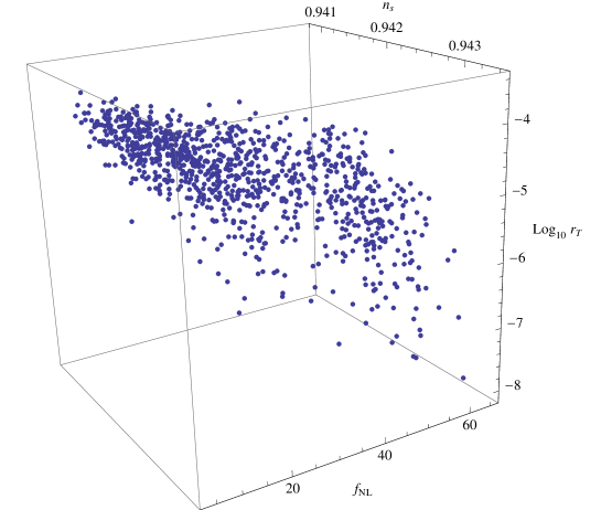
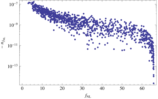
which is the same as that in [5]. For N60similar-to-or-equalssubscript𝑁60N_{*}\simeq 60, ns0.942similar-to-or-equalssubscript𝑛𝑠0.942n_{s}\simeq 0.942. The numerical results for NNtot60similar-to-or-equalssubscript𝑁subscript𝑁𝑡𝑜𝑡similar-to-or-equals60N_{*}\simeq N_{tot}\simeq 60 and f=1/2𝑓12f=1/2 are illustrated in Fig. 1.

Refer to caption
Refer to caption
Figure 1: The observables of axion N-flation with the same potential for different inflatons. Here f=1/2𝑓12f=1/2 and the initial conditions of αisubscript𝛼𝑖\alpha_{i} is assumed to be the uniform distribution.

The spectral index of scalar power spectrum is nicely compatible with the estimation, and the tensor-scalar ratio is roughly 𝒪(105103)𝒪similar-tosuperscript105superscript103{\cal O}(10^{-5}\sim 10^{-3}). As long as Nfsubscript𝑁𝑓N_{f} is large enough, from Eqs. (44) and (45), both rTsubscript𝑟𝑇r_{T} and fNLsubscript𝑓𝑁𝐿f_{NL} are proportional to 1/f21superscript𝑓21/f^{2}. From the numerical results, we find that fNLsubscript𝑓𝑁𝐿f_{NL} is bounded from above, namely

fNL5π23f2.less-than-or-similar-tosubscript𝑓𝑁𝐿5superscript𝜋23superscript𝑓2\displaystyle f_{NL}\lesssim{5\pi^{2}\over 3f^{2}}. (53)

For f1less-than-or-similar-to𝑓1f\lesssim 1, the value of fNLsubscript𝑓𝑁𝐿f_{NL} can be of order 𝒪(10)𝒪10{\cal O}(10) which is large enough to be detected in the near future, but its tilt nfNLsubscript𝑛subscript𝑓𝑁𝐿n_{f_{NL}} (𝒪(107)𝒪(1014))similar-to𝒪superscript107𝒪superscript1014(-{\cal O}(10^{-7})\sim-{\cal O}(10^{-14})) is too small to be detected in this case.

3.1.2 A few inflatons stays around the hilltop

In [5], the authors proposed an alternative way to achieve a large fNLsubscript𝑓𝑁𝐿f_{NL}. Roughly speaking, the summation of the function which is proportional to 1/ϵi1subscriptitalic-ϵ𝑖1/\epsilon_{i} is dominated by those fields with the smallest ϵisubscriptitalic-ϵ𝑖\epsilon_{i}, or equivalently staying around the hilltop. Suppose some number N¯¯𝑁\bar{N} of fields have roughly comparable ϵisubscriptitalic-ϵ𝑖\epsilon_{i}, of order ϵ¯¯italic-ϵ\bar{\epsilon} which is related to the angle α¯¯𝛼\bar{\alpha} by

ϵ¯π2f2(1+cosα¯)π22f2(πα¯)2,similar-to-or-equals¯italic-ϵsuperscript𝜋2superscript𝑓21¯𝛼similar-to-or-equalssuperscript𝜋22superscript𝑓2superscript𝜋¯𝛼2\displaystyle\bar{\epsilon}\simeq{\pi^{2}\over f^{2}}(1+\cos{\bar{\alpha}})\simeq{\pi^{2}\over 2f^{2}}(\pi-{\bar{\alpha}})^{2}, (54)

with (πα¯)1much-less-than𝜋¯𝛼1(\pi-{\bar{\alpha}})\ll 1. In this case, Pζsubscript𝑃𝜁P_{\zeta}, rTsubscript𝑟𝑇r_{T}, and fNLsubscript𝑓𝑁𝐿f_{NL} becomes

Pζsubscript𝑃𝜁\displaystyle P_{\zeta} similar-to-or-equals\displaystyle\simeq H28π2N¯ϵ¯H2N¯f24π4(πα¯)2,similar-to-or-equalssuperscript𝐻28superscript𝜋2¯𝑁¯italic-ϵsuperscript𝐻2¯𝑁superscript𝑓24superscript𝜋4superscript𝜋¯𝛼2\displaystyle{H^{2}\over 8\pi^{2}}{{\bar{N}}\over{\bar{\epsilon}}}\simeq{H^{2}{\bar{N}}f^{2}\over 4\pi^{4}(\pi-{\bar{\alpha}})^{2}}, (55)
rTsubscript𝑟𝑇\displaystyle r_{T} similar-to-or-equals\displaystyle\simeq 16ϵ¯N¯8π2N¯f2(πα¯)2,similar-to-or-equals16¯italic-ϵ¯𝑁8superscript𝜋2¯𝑁superscript𝑓2superscript𝜋¯𝛼2\displaystyle{16{\bar{\epsilon}}\over{\bar{N}}}\simeq{8\pi^{2}\over{\bar{N}}f^{2}}(\pi-{\bar{\alpha}})^{2}, (56)
fNLsubscript𝑓𝑁𝐿\displaystyle f_{NL} similar-to-or-equals\displaystyle\simeq 5π23N¯f2.5superscript𝜋23¯𝑁superscript𝑓2\displaystyle{5\pi^{2}\over 3{\bar{N}}f^{2}}. (57)

Considering N¯1¯𝑁1{\bar{N}}\geq 1,

fNL5π23f2,less-than-or-similar-tosubscript𝑓𝑁𝐿5superscript𝜋23superscript𝑓2\displaystyle f_{NL}\lesssim{5\pi^{2}\over 3f^{2}}, (58)

which is the same as that in Sec. 3.1.1. Now the spectral index of fNLsubscript𝑓𝑁𝐿f_{NL} is given by

nfNL1+cosα¯2(1ns2ϵH),similar-to-or-equalssubscript𝑛subscript𝑓𝑁𝐿1¯𝛼21subscript𝑛𝑠2subscriptitalic-ϵ𝐻\displaystyle n_{f_{NL}}\simeq-{1+\cos{\bar{\alpha}}\over 2}(1-n_{s}-2\epsilon_{H}), (59)

which is much smaller than (1ns2ϵH)1subscript𝑛𝑠2subscriptitalic-ϵ𝐻(1-n_{s}-2\epsilon_{H}). So the spectral index of fNLsubscript𝑓𝑁𝐿f_{NL} is undetectable in this case as well.

Because the potential become very flat around the hilltop, one may worry that the classical motions of those inflatons staying around the hilltop are not reliable. Requiring that the classical motion of inflaton ϕ¯=fα¯/2π¯italic-ϕ𝑓¯𝛼2𝜋{\bar{\phi}}=f{\bar{\alpha}}/2\pi per Hubble time be not less than its quantum fluctuation H/2π𝐻2𝜋H/2\pi yields

(πα¯)3fH34π2Λ4=2ξ1Hf,greater-than-or-equivalent-to𝜋¯𝛼3𝑓superscript𝐻34superscript𝜋2superscriptΛ42superscript𝜉1𝐻𝑓\displaystyle(\pi-{\bar{\alpha}})\gtrsim{3fH^{3}\over 4\pi^{2}\Lambda^{4}}=2\xi^{-1}{H\over f}, (60)

where ξ=8π2Λ4/(3H2f2)=(1ns2ϵH)1𝜉8superscript𝜋2superscriptΛ43superscript𝐻2superscript𝑓21subscript𝑛𝑠2subscriptitalic-ϵ𝐻much-less-than1\xi=8\pi^{2}\Lambda^{4}/(3H^{2}f^{2})=(1-n_{s}-2\epsilon_{H})\ll 1. 222In [5], the authors consider |ϕhilltopϕ¯|H/2πgreater-than-or-equivalent-tosubscriptitalic-ϕ𝑖𝑙𝑙𝑡𝑜𝑝¯italic-ϕ𝐻2𝜋|\phi_{hilltop}-{\bar{\phi}}|\gtrsim H/2\pi, namely (πα¯)H/fgreater-than-or-equivalent-to𝜋¯𝛼𝐻𝑓(\pi-{\bar{\alpha}})\gtrsim H/f, which is much looser than what we require, where ϕhilltopf/2subscriptitalic-ϕ𝑖𝑙𝑙𝑡𝑜𝑝𝑓2\phi_{hilltop}\equiv f/2. On the other hand, from (55), (πα¯)𝜋¯𝛼(\pi-{\bar{\alpha}}) can be estimated by

(πα¯)=N¯Hf2π2Δ,𝜋¯𝛼¯𝑁𝐻𝑓2superscript𝜋2subscriptΔ\displaystyle(\pi-{\bar{\alpha}})={\sqrt{\bar{N}}Hf\over 2\pi^{2}\Delta_{\cal R}}, (61)

where Δ=PζsubscriptΔsubscript𝑃𝜁\Delta_{\cal R}=\sqrt{P_{\zeta}}. Therefore

N¯f24π2Δξ.greater-than-or-equivalent-to¯𝑁superscript𝑓24superscript𝜋2subscriptΔ𝜉\displaystyle\sqrt{\bar{N}}f^{2}\gtrsim{4\pi^{2}\Delta_{\cal R}\over\xi}. (62)

Taking Eq.(57) into account, fNLsubscript𝑓𝑁𝐿f_{NL} is bounded from above by

fNL512ξΔ/N¯.less-than-or-similar-tosubscript𝑓𝑁𝐿/512𝜉subscriptΔ¯𝑁\displaystyle f_{NL}\lesssim{5\over 12}{\xi\over\Delta_{\cal R}}\left/\sqrt{\bar{N}}\right.. (63)

WMAP normalization [27] implies Pζ=Δ2=2.461×10⁹subscript𝑃𝜁superscriptsubscriptΔ22.461superscript109P_{\zeta}=\Delta_{\cal R}^{2}=2.461\times 10^{-9}, and then fNL8×103ξ/N¯less-than-or-similar-tosubscript𝑓𝑁𝐿8superscript103𝜉¯𝑁f_{NL}\lesssim 8\times 10^{3}\xi/\sqrt{\bar{N}}. Since ξ𝒪(102)less-than-or-similar-to𝜉𝒪superscript102\xi\lesssim{\cal O}(10^{-2}), fNL80/N¯less-than-or-similar-tosubscript𝑓𝑁𝐿80¯𝑁f_{NL}\lesssim 80/\sqrt{\bar{N}}. The value of fNLsubscript𝑓𝑁𝐿f_{NL} cannot be very large in this case.

3.2 Axion N-flation with different potential for different inflatons

In this subsection, we consider a class of axion N-flation in which Λi=ΛsubscriptΛ𝑖Λ\Lambda_{i}=\Lambda for ifor-all𝑖\forall\ i, but the decay constants can be different for different inflatons. For simplicity, we only focus on the cases with only two different decay constants.

3.2.1 One inflaton with different decay constant stays around the hilltop

In this subsubsection we consider a model with potentials

V(ϕi)𝑉subscriptitalic-ϕ𝑖\displaystyle V(\phi_{i}) =\displaystyle= Λ4(1cosαi),superscriptΛ41subscript𝛼𝑖\displaystyle\Lambda^{4}(1-\cos\alpha_{i}), (64)
V(ϕ¯)𝑉¯italic-ϕ\displaystyle V(\bar{\phi}) =\displaystyle= Λ4(1cosα¯),superscriptΛ41¯𝛼\displaystyle\Lambda^{4}(1-\cos{\bar{\alpha}}), (65)

where αi=2πϕi/fsubscript𝛼𝑖2𝜋subscriptitalic-ϕ𝑖𝑓\alpha_{i}=2\pi\phi_{i}/f for i=1,2,,Nf𝑖12subscript𝑁𝑓i=1,2,...,N_{f} and α¯=2πϕ¯/f¯¯𝛼2𝜋¯italic-ϕ¯𝑓\bar{\alpha}=2\pi{\bar{\phi}}/{\bar{f}}. Here f𝑓f is assumed to be different from f¯¯𝑓\bar{f}. We consider Nf1much-greater-thansubscript𝑁𝑓1N_{f}\gg 1 and the initial values of αisubscript𝛼𝑖\alpha_{i} satisfy a uniform distribution. 333Thank C. T. Byrnes for the helpful discussion. The total number of e-folds before the end of inflation is given by

Ntotln22π2f2Nf+f¯24π2ln21+cosα¯.similar-to-or-equalssubscript𝑁𝑡𝑜𝑡22superscript𝜋2superscript𝑓2subscript𝑁𝑓superscript¯𝑓24superscript𝜋221¯𝛼\displaystyle N_{tot}\simeq{\ln 2\over 2\pi^{2}}f^{2}N_{f}+{{\bar{f}}^{2}\over 4\pi^{2}}\ln{2\over 1+\cos{\bar{\alpha}}}. (66)

We assume ϕ¯¯italic-ϕ\bar{\phi} stays around the hilltop of its potential. Requiring that the classical motion of inflaton ϕ¯¯italic-ϕ{\bar{\phi}} is reliable leads to

(πα¯ini)3f¯H34π2Λ4,greater-than-or-equivalent-to𝜋subscript¯𝛼𝑖𝑛𝑖3¯𝑓superscript𝐻34superscript𝜋2superscriptΛ4\displaystyle(\pi-{\bar{\alpha}}_{ini})\gtrsim{3{\bar{f}}H^{3}\over 4\pi^{2}\Lambda^{4}}, (67)

where α¯inisubscript¯𝛼𝑖𝑛𝑖{\bar{\alpha}}_{ini} denotes the initial value of α¯¯𝛼{\bar{\alpha}}.

In this model, the Hubble parameter is roughly related to ΛΛ\Lambda by H2NfΛ4/3similar-to-or-equalssuperscript𝐻2subscript𝑁𝑓superscriptΛ43H^{2}\simeq N_{f}\Lambda^{4}/3. Because the inflaton staying around the hilltop almost does not move, we also have

ϵHln22/(Ntotf¯22π2ln2πα¯).similar-to-or-equalssubscriptitalic-ϵ𝐻/22subscript𝑁𝑡𝑜𝑡superscript¯𝑓22superscript𝜋22𝜋¯𝛼\epsilon_{H}\simeq{\ln 2\over 2}\left/\left(N_{tot}-{{\bar{f}}^{2}\over 2\pi^{2}}\ln{2\over\pi-\bar{\alpha}}\right)\right.\ . (68)

The spectral index of power spectrum and fNLsubscript𝑓𝑁𝐿f_{NL} become

nssubscript𝑛𝑠\displaystyle n_{s} similar-to-or-equals\displaystyle\simeq 1ln2Ntotf¯22π2ln2πα¯[1+4cr(Nf)Nf+4(πα¯)2cr(Nf)Nf+(f¯/f)24(πα¯)2],12subscript𝑁𝑡𝑜𝑡superscript¯𝑓22superscript𝜋22𝜋¯𝛼delimited-[]14subscript𝑐𝑟subscript𝑁𝑓subscript𝑁𝑓4superscript𝜋¯𝛼2subscript𝑐𝑟subscript𝑁𝑓subscript𝑁𝑓superscript¯𝑓𝑓24superscript𝜋¯𝛼2\displaystyle 1-{\ln 2\over N_{tot}-{{\bar{f}}^{2}\over 2\pi^{2}}\ln{2\over\pi-\bar{\alpha}}}\left[1+4{c_{r}(N_{f})N_{f}+{4\over(\pi-\bar{\alpha})^{2}}\over c_{r}(N_{f})N_{f}+(\bar{f}/f)^{2}{4\over(\pi-\bar{\alpha})^{2}}}\right], (69)
nfNLsubscript𝑛subscript𝑓𝑁𝐿\displaystyle n_{f_{NL}} similar-to-or-equals\displaystyle\simeq 8ln2Ntotf¯22π2ln2πα¯[cr(Nf)Nf+4(πα¯)2cr(Nf)Nf+(f¯/f)24(πα¯)2dr(Nf)Nf+8(πα¯)4dr(Nf)Nf+(f¯/f)28(πα¯)4],82subscript𝑁𝑡𝑜𝑡superscript¯𝑓22superscript𝜋22𝜋¯𝛼delimited-[]subscript𝑐𝑟subscript𝑁𝑓subscript𝑁𝑓4superscript𝜋¯𝛼2subscript𝑐𝑟subscript𝑁𝑓subscript𝑁𝑓superscript¯𝑓𝑓24superscript𝜋¯𝛼2subscript𝑑𝑟subscript𝑁𝑓subscript𝑁𝑓8superscript𝜋¯𝛼4subscript𝑑𝑟subscript𝑁𝑓subscript𝑁𝑓superscript¯𝑓𝑓28superscript𝜋¯𝛼4\displaystyle{8\ln 2\over N_{tot}-{{\bar{f}}^{2}\over 2\pi^{2}}\ln{2\over\pi-\bar{\alpha}}}\left[{c_{r}(N_{f})N_{f}+{4\over(\pi-\bar{\alpha})^{2}}\over c_{r}(N_{f})N_{f}+(\bar{f}/f)^{2}{4\over(\pi-\bar{\alpha})^{2}}}-{d_{r}(N_{f})N_{f}+{8\over(\pi-\bar{\alpha})^{4}}\over d_{r}(N_{f})N_{f}+(\bar{f}/f)^{2}{8\over(\pi-\bar{\alpha})^{4}}}\right],

where

cr(N)=1Ni=1N1cosαi1+cosαi,anddr(N)=1Ni=1N1cosαi(1+cosαi)2,formulae-sequencesubscript𝑐𝑟𝑁1𝑁superscriptsubscript𝑖1𝑁1subscript𝛼𝑖1subscript𝛼𝑖andsubscript𝑑𝑟𝑁1𝑁superscriptsubscript𝑖1𝑁1subscript𝛼𝑖superscript1subscript𝛼𝑖2\displaystyle c_{r}(N)={1\over N}\sum_{i=1}^{N}{1-\cos\alpha_{i}\over 1+\cos\alpha_{i}},\ \hbox{and}\ d_{r}(N)={1\over N}\sum_{i=1}^{N}{1-\cos\alpha_{i}\over(1+\cos\alpha_{i})^{2}}, (71)

which depend on the total number of points and the random choice of the series ‘r𝑟r’ for αi[0,π]subscript𝛼𝑖0𝜋\alpha_{i}\in[0,\pi].

Similar to Sec. 3.1.1, we consider that the total number of e-folds corresponds to the CMB scale, namely NNtot60similar-to-or-equalssubscript𝑁subscript𝑁𝑡𝑜𝑡similar-to-or-equals60N_{*}\simeq N_{tot}\simeq 60. Considering f¯1less-than-or-similar-to¯𝑓1{\bar{f}}\lesssim 1, the total number of e-fold is mainly contributed by ϕisubscriptitalic-ϕ𝑖\phi_{i} for i=1,2,,Nf𝑖12subscript𝑁𝑓i=1,2,...,N_{f}. If f=f¯𝑓¯𝑓f={\bar{f}}, ns15ln2/Nsimilar-to-or-equalssubscript𝑛𝑠152subscript𝑁n_{s}\simeq 1-5\ln 2/N_{*} and nfNL0similar-to-or-equalssubscript𝑛subscript𝑓𝑁𝐿0n_{f_{NL}}\simeq 0 which are consistent with the results in Sec. 3.1.1.

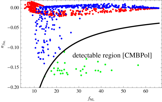
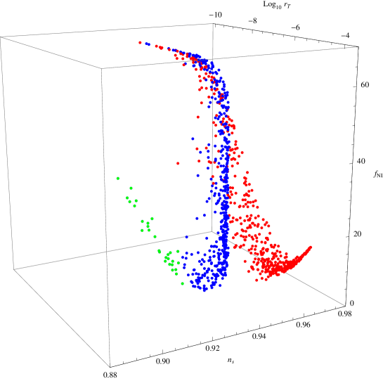
For f¯<f¯𝑓𝑓\bar{f}<f, the second term in the bracket of Eq. (69) is larger than 4 and then ns15ln2/Nless-than-or-similar-tosubscript𝑛𝑠152subscript𝑁n_{s}\lesssim 1-5\ln 2/N_{*}. For f¯>f¯𝑓𝑓\bar{f}>f, we find ns15ln2/Ngreater-than-or-equivalent-tosubscript𝑛𝑠152subscript𝑁n_{s}\gtrsim 1-5\ln 2/N_{*}. In general, it is difficult to get the analytical estimation for the model with ff¯𝑓¯𝑓f\neq\bar{f}, but we can expect that the results should be quite different the model with the same decay constants. The numerical results are showed in Fig. 2.
Refer to caption
Refer to caption
Figure 2: The observables of axion N-flation with different decay constants. Here we adopt f=1/2𝑓12f=1/2 and (πα¯ini)/π=2×104𝜋subscript¯𝛼𝑖𝑛𝑖𝜋2superscript104(\pi-{\bar{\alpha}}_{ini})/\pi=2\times 10^{-4}. The blue and green dots correspond to f¯=1/4¯𝑓14{\bar{f}}=1/4 and the red dots corresponds to f¯=1¯𝑓1{\bar{f}}=1. The green dots illustrate the case with detectable scale dependence of fNLsubscript𝑓𝑁𝐿f_{NL}.

Here we keep f=1/2𝑓12f=1/2 and (πα¯ini)/π=2×104𝜋subscript¯𝛼𝑖𝑛𝑖𝜋2superscript104(\pi-{\bar{\alpha}}_{ini})/\pi=2\times 10^{-4} fixed and explore the results for two choices of f¯¯𝑓\bar{f}. From Fig. 2, we see that a detectable negative nfNLsubscript𝑛subscript𝑓𝑁𝐿n_{f_{NL}} is possibly generated for f¯=1/4¯𝑓14{\bar{f}}=1/4. We also check the requirement in (67) which is satisfied as long as (πα¯)/π2×105greater-than-or-equivalent-to𝜋¯𝛼𝜋2superscript105(\pi-{\bar{\alpha}})/\pi\gtrsim 2\times 10^{-5} for f¯=1/4¯𝑓14{\bar{f}}=1/4. Unfortunately, the spectral index ns(0.91)annotatedsubscript𝑛𝑠less-than-or-similar-toabsent0.91n_{s}\ (\lesssim 0.91) in the case with detectable nfNLsubscript𝑛subscript𝑓𝑁𝐿n_{f_{NL}} is small compared to WMAP 7yr data [27] (ns=0.968±0.012)subscript𝑛𝑠plus-or-minus0.9680.012(n_{s}=0.968\pm 0.012). See the green dots in Fig. 2. For f¯=1¯𝑓1{\bar{f}}=1, the spectral index can fit the WMAP 7yr data nicely, but the scale dependence of fNLsubscript𝑓𝑁𝐿f_{NL} becomes negligibly small. See the red dots in Fig. 2. This setup indicates that a large nfNLsubscript𝑛subscript𝑓𝑁𝐿n_{f_{NL}} can be achieved in axion N-flation.

3.2.2 A general axion N-flation with two kinds of inflatons

In this subsubsection we consider a more general axion N-flation model in which there are two kinds of inflatons who have different decay constants,

V1(ϕ1,i)subscript𝑉1subscriptitalic-ϕ1𝑖\displaystyle V_{1}(\phi_{1,i}) =\displaystyle= Λ4(1cosα1,i),superscriptΛ41subscript𝛼1𝑖\displaystyle\Lambda^{4}(1-\cos\alpha_{1,i}), (72)
V2(ϕ2,j)subscript𝑉2subscriptitalic-ϕ2𝑗\displaystyle V_{2}(\phi_{2,j}) =\displaystyle= Λ4(1cosα2,j),superscriptΛ41subscript𝛼2𝑗\displaystyle\Lambda^{4}(1-\cos\alpha_{2,j}), (73)

where α1,i=2πϕ1,i/f1subscript𝛼1𝑖2𝜋subscriptitalic-ϕ1𝑖subscript𝑓1\alpha_{1,i}=2\pi\phi_{1,i}/f_{1} for i=1,2,,N1𝑖12subscript𝑁1i=1,2,...,N_{1}, and α2,j=2πϕ2,j/f2subscript𝛼2𝑗2𝜋subscriptitalic-ϕ2𝑗subscript𝑓2\alpha_{2,j}=2\pi\phi_{2,j}/f_{2} for j=1,2,,N2𝑗12subscript𝑁2j=1,2,...,N_{2}. Here f1subscript𝑓1f_{1} is assumed to be different from f2subscript𝑓2f_{2}. We also consider N1,N21much-greater-thansubscript𝑁1subscript𝑁21N_{1},\ N_{2}\gg 1 and the initial values of α1,isubscript𝛼1𝑖\alpha_{1,i} and α2,jsubscript𝛼2𝑗\alpha_{2,j} satisfy a uniform distribution respectively. In this model the total number of e-folds before the end of inflation is given by

Ntotln22π2(f12N1+f22N2).similar-to-or-equalssubscript𝑁𝑡𝑜𝑡22superscript𝜋2superscriptsubscript𝑓12subscript𝑁1superscriptsubscript𝑓22subscript𝑁2\displaystyle N_{tot}\simeq{\ln 2\over 2\pi^{2}}(f_{1}^{2}N_{1}+f_{2}^{2}N_{2}). (74)

In this model, the Hubble parameter is related to ΛΛ\Lambda by H2=(N1+N2)Λ4/3superscript𝐻2subscript𝑁1subscript𝑁2superscriptΛ43H^{2}=(N_{1}+N_{2})\Lambda^{4}/3 and the slow-roll parameter is given by

ϵH=π2(N1+N2)2(N1/f12+N2/f22).subscriptitalic-ϵ𝐻superscript𝜋2superscriptsubscript𝑁1subscript𝑁22subscript𝑁1superscriptsubscript𝑓12subscript𝑁2superscriptsubscript𝑓22\displaystyle\epsilon_{H}={\pi^{2}\over(N_{1}+N_{2})^{2}}\left(N_{1}/f_{1}^{2}+N_{2}/f_{2}^{2}\right). (75)

Similarly, we can also derive the spectral index of power spectrum and fNLsubscript𝑓𝑁𝐿f_{NL}, namely

nssubscript𝑛𝑠\displaystyle n_{s} similar-to-or-equals\displaystyle\simeq 12π2(N1+N2)2(N1f12+N2f22)8π2N1+N2cr1(N1)N1+cr2(N2)N2cr1(N1)f12N1+cr2(N2)f22N2,12superscript𝜋2superscriptsubscript𝑁1subscript𝑁22subscript𝑁1superscriptsubscript𝑓12subscript𝑁2superscriptsubscript𝑓228superscript𝜋2subscript𝑁1subscript𝑁2subscript𝑐subscript𝑟1subscript𝑁1subscript𝑁1subscript𝑐subscript𝑟2subscript𝑁2subscript𝑁2subscript𝑐subscript𝑟1subscript𝑁1superscriptsubscript𝑓12subscript𝑁1subscript𝑐subscript𝑟2subscript𝑁2superscriptsubscript𝑓22subscript𝑁2\displaystyle 1-{2\pi^{2}\over(N_{1}+N_{2})^{2}}\left({N_{1}\over f_{1}^{2}}+{N_{2}\over f_{2}^{2}}\right)-{8\pi^{2}\over N_{1}+N_{2}}{c_{r_{1}}(N_{1})N_{1}+c_{r_{2}}(N_{2})N_{2}\over c_{r_{1}}(N_{1})f_{1}^{2}N_{1}+c_{r_{2}}(N_{2})f_{2}^{2}N_{2}}, (76)
nfNLsubscript𝑛subscript𝑓𝑁𝐿\displaystyle n_{f_{NL}} similar-to-or-equals\displaystyle\simeq 16π2N1+N2[cr1(N1)N1+cr2(N2)N2cr1(N1)f12N1+cr2(N2)f22N2dr1(N1)N1+dr2(N2)N2dr1(N1)f12N1+dr2(N2)f22N2].16superscript𝜋2subscript𝑁1subscript𝑁2delimited-[]subscript𝑐subscript𝑟1subscript𝑁1subscript𝑁1subscript𝑐subscript𝑟2subscript𝑁2subscript𝑁2subscript𝑐subscript𝑟1subscript𝑁1superscriptsubscript𝑓12subscript𝑁1subscript𝑐subscript𝑟2subscript𝑁2superscriptsubscript𝑓22subscript𝑁2subscript𝑑subscript𝑟1subscript𝑁1subscript𝑁1subscript𝑑subscript𝑟2subscript𝑁2subscript𝑁2subscript𝑑subscript𝑟1subscript𝑁1superscriptsubscript𝑓12subscript𝑁1subscript𝑑subscript𝑟2subscript𝑁2superscriptsubscript𝑓22subscript𝑁2\displaystyle{16\pi^{2}\over N_{1}+N_{2}}\left[{c_{r_{1}}(N_{1})N_{1}+c_{r_{2}}(N_{2})N_{2}\over c_{r_{1}}(N_{1})f_{1}^{2}N_{1}+c_{r_{2}}(N_{2})f_{2}^{2}N_{2}}-{d_{r_{1}}(N_{1})N_{1}+d_{r_{2}}(N_{2})N_{2}\over d_{r_{1}}(N_{1})f_{1}^{2}N_{1}+d_{r_{2}}(N_{2})f_{2}^{2}N_{2}}\right].\quad (77)

Again, if f1=f2subscript𝑓1subscript𝑓2f_{1}=f_{2}, the scale dependence of fNLsubscript𝑓𝑁𝐿f_{NL} is negligibly small and our results recover those in Sec. 3.1.1.

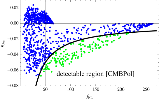
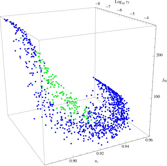
For the case with f1f2subscript𝑓1subscript𝑓2f_{1}\neq f_{2}, we need to adopt numerical method to explore it. Considering NNtot60similar-to-or-equalssubscript𝑁subscript𝑁𝑡𝑜𝑡similar-to-or-equals60N_{*}\simeq N_{tot}\simeq 60, our numerical results are illustrated in Fig. 3.
Refer to caption
Refer to caption
Figure 3: The observables of a general axion N-flation with different decay constants. Here we adopt f1=1/2subscript𝑓112f_{1}=1/2 and f2=1/4subscript𝑓214f_{2}=1/4. The green dots illustrate the case with detectable scale dependence of fNLsubscript𝑓𝑁𝐿f_{NL}.

Here we adopt f1=1/2subscript𝑓112f_{1}=1/2, N1=4800subscript𝑁14800N_{1}=4800, f2=1/4subscript𝑓214f_{2}=1/4 and N2=8000subscript𝑁28000N_{2}=8000. We see that a detectable scale dependence of fNLsubscript𝑓𝑁𝐿f_{NL} can be obtained.

4 Discussions

In this paper we work out the spectral index of fNLsubscript𝑓𝑁𝐿f_{NL} in general N-flation model by adopting the horizon-crossing approximation. For an instance, we focus on the axion N-flation proposed in [5] and we find that fNLsubscript𝑓𝑁𝐿f_{NL} can be large enough to be detected in the near future.
\bullet All inflatons have the same potential. In the case with the total number of e-folds corresponding to the CMB scale, fNLsubscript𝑓𝑁𝐿f_{NL} is roughly of order 𝒪(10)𝒪10{\cal O}(10) for a uniform distribution of initial angles if the decay constant f𝑓f is around the Planck scale. Our numerical results indicate that fNLsubscript𝑓𝑁𝐿f_{NL} is bounded from above by 5π2/3f25superscript𝜋23superscript𝑓25\pi^{2}/3f^{2}, and τNL(2π/f)2/3fNL5/3similar-to-or-equalssubscript𝜏𝑁𝐿superscript2𝜋𝑓23superscriptsubscript𝑓𝑁𝐿53\tau_{NL}\simeq(2\pi/f)^{2/3}f_{NL}^{5/3}. Another way to obtain a large fNLsubscript𝑓𝑁𝐿f_{NL} is that a few inflatons stay around the hilltop and the summations in the formula of fNLsubscript𝑓𝑁𝐿f_{NL} is mainly contributed by these inflatons. Typically fNLsubscript𝑓𝑁𝐿f_{NL} is less than one hundred in the second case. In both cases the tilt of fNLsubscript𝑓𝑁𝐿f_{NL} is negligibly small. The smallness of nfNLsubscript𝑛subscript𝑓𝑁𝐿n_{f_{NL}} in these two case comes from the accident cancellation in nmulti,isubscript𝑛𝑚𝑢𝑙𝑡𝑖𝑖n_{multi,i} because all inflatons have the same potential.
\bullet Different inflatons have different decay constants. In this kind of model, the accident cancellation in nmulti,isubscript𝑛𝑚𝑢𝑙𝑡𝑖𝑖n_{multi,i} does not happen and a negative detectable nfNLsubscript𝑛subscript𝑓𝑁𝐿n_{f_{NL}} can be obtained. It implies that a scale independent fNLsubscript𝑓𝑁𝐿f_{NL} is not generic prediction of N-flation. A more general axion N-flation is left to be studied in the future.

In addition, we also study the trispectrum for N-flation in the Appendix. A. We find that there is a universal relation between gNLsubscript𝑔𝑁𝐿g_{NL} and τNLsubscript𝜏𝑁𝐿\tau_{NL}, namely gNL25τNL/27similar-to-or-equalssubscript𝑔𝑁𝐿25subscript𝜏𝑁𝐿27g_{NL}\simeq 25\tau_{NL}/27, for the cases with large fNLsubscript𝑓𝑁𝐿f_{NL}. But the relation between fNLsubscript𝑓𝑁𝐿f_{NL} and τNLsubscript𝜏𝑁𝐿\tau_{NL} depends on detail of the model.

If there is only one inflaton field, the axion N-flation becomes natural inflation. The slow-roll parameters are roughly given by Mp2/f2superscriptsubscript𝑀𝑝2superscript𝑓2M_{p}^{2}/f^{2} and then the slow-roll conditions are satisfied if f>Mp𝑓subscript𝑀𝑝f>M_{p}. However such a large decay constant cannot be achieved in some fundamental theories, such as string theory [28, 29]. In [30] the N-flation is supposed to realize a slow-roll inflation even when f<Mp𝑓subscript𝑀𝑝f<M_{p} by calling multi inflaton fields. On the other hand, in [31] we proposed a conjecture that the effective gravity scale should be ΛG=Mp/NfsubscriptΛ𝐺subscript𝑀𝑝subscript𝑁𝑓\Lambda_{G}=M_{p}/\sqrt{N_{f}} for the case with multi scalar fields, not Mpsubscript𝑀𝑝M_{p}. If the decay constant of axion field is required to be smaller than ΛGsubscriptΛ𝐺\Lambda_{G}, namely Nff2<1subscript𝑁𝑓superscript𝑓21N_{f}f^{2}<1, the total number of e-folds is less than one and the axion N-flation fails.

Acknowledgments

We would like to thank S. A. Kim and A. R. Liddle for useful discussions. QGH is supported by the project of Knowledge Innovation Program of Chinese Academy of Science and a grant from NSFC.

Appendix A The trispectrum in N-flation

From Eq. (1), the size of trispectrum is characterized by two parameters τNLsubscript𝜏𝑁𝐿\tau_{NL} and gNLsubscript𝑔𝑁𝐿g_{NL} which are defined by

τNLsubscript𝜏𝑁𝐿\displaystyle\tau_{NL} =\displaystyle= i,j,kN,ijN,ikN,jN,k/(lN,l2)3,\displaystyle\sum_{i,j,k}N_{,ij}N_{,ik}N_{,j}N_{,k}\left/(\sum_{l}N_{,l}^{2})^{3}\right., (78)
gNLsubscript𝑔𝑁𝐿\displaystyle g_{NL} =\displaystyle= 2554i,j,kN,ijkN,iN,jN,k/(lN,l2)3.\displaystyle{25\over 54}\sum_{i,j,k}N_{,ijk}N_{,i}N_{,j}N_{,k}\left/(\sum_{l}N_{,l}^{2})^{3}\right.. (79)

For N-flation, the above two equations are simplified to be

τNLsubscript𝜏𝑁𝐿\displaystyle\tau_{NL} =\displaystyle= iN,ii2N,i2/(lN,l2)3,\displaystyle\sum_{i}N_{,ii}^{2}N_{,i}^{2}\left/(\sum_{l}N_{,l}^{2})^{3}\right., (80)
gNLsubscript𝑔𝑁𝐿\displaystyle g_{NL} =\displaystyle= 2554iN,iiiN,i3/(lN,l2)3,\displaystyle{25\over 54}\sum_{i}N_{,iii}N_{,i}^{3}\left/(\sum_{l}N_{,l}^{2})^{3}\right., (81)

where

N,iii=2ViVi′′2Vi3Vi′′ViViVi′′′Vi2.\displaystyle N_{,iii}=2{V_{i}V_{i}^{\prime\prime 2}\over V_{i}^{\prime 3}}-{V_{i}^{\prime\prime}\over V_{i}^{\prime}}-{V_{i}V_{i}^{\prime\prime\prime}\over V_{i}^{\prime 2}}. (82)

We remind the readers that the value of τNLsubscript𝜏𝑁𝐿\tau_{NL} is bounded from below by (65fNL)2superscript65subscript𝑓𝑁𝐿2({6\over 5}f_{NL})^{2}. For the axion N-flation, we have

N,iii=2πfisinαi(1+cosαi)2.\displaystyle N_{,iii}={2\pi\over f_{i}}{\sin\alpha_{i}\over(1+\cos\alpha_{i})^{2}}. (83)

Therefore

τNLsubscript𝜏𝑁𝐿\displaystyle\tau_{NL} =\displaystyle= ifi24π21cosαi(1+cosαi)3/(jfj24π21cosαj1+cosαj)3,subscript𝑖/superscriptsubscript𝑓𝑖24superscript𝜋21subscript𝛼𝑖superscript1subscript𝛼𝑖3superscriptsubscript𝑗superscriptsubscript𝑓𝑗24superscript𝜋21subscript𝛼𝑗1subscript𝛼𝑗3\displaystyle\sum_{i}{f_{i}^{2}\over 4\pi^{2}}{1-\cos\alpha_{i}\over(1+\cos\alpha_{i})^{3}}\left/\left(\sum_{j}{f_{j}^{2}\over 4\pi^{2}}{1-\cos\alpha_{j}\over 1+\cos\alpha_{j}}\right)^{3}\right., (84)
gNLsubscript𝑔𝑁𝐿\displaystyle g_{NL} =\displaystyle= 2554ifi24π2(1cosαi)2(1+cosαi)3/(jfj24π21cosαj1+cosαj)3.2554subscript𝑖/superscriptsubscript𝑓𝑖24superscript𝜋2superscript1subscript𝛼𝑖2superscript1subscript𝛼𝑖3superscriptsubscript𝑗superscriptsubscript𝑓𝑗24superscript𝜋21subscript𝛼𝑗1subscript𝛼𝑗3\displaystyle{25\over 54}\sum_{i}{f_{i}^{2}\over 4\pi^{2}}{(1-\cos\alpha_{i})^{2}\over(1+\cos\alpha_{i})^{3}}\left/\left(\sum_{j}{f_{j}^{2}\over 4\pi^{2}}{1-\cos\alpha_{j}\over 1+\cos\alpha_{j}}\right)^{3}\right.. (85)

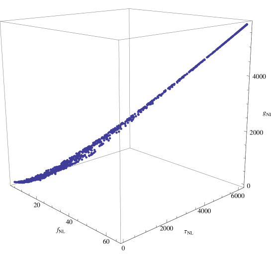
For the case with fi=fsubscript𝑓𝑖𝑓f_{i}=f for ifor-all𝑖\forall\ i, both τNLsubscript𝜏𝑁𝐿\tau_{NL} and gNLsubscript𝑔𝑁𝐿g_{NL} are proportional to 1/f41superscript𝑓41/f^{4}. Similar to Sec. 3.1.1, we consider NNtot60similar-to-or-equalssubscript𝑁subscript𝑁𝑡𝑜𝑡similar-to-or-equals60N_{*}\simeq N_{tot}\simeq 60 and the numerical results for f=1/2𝑓12f=1/2 are showed in Fig. 4.

Refer to caption
Figure 4: The non-Gaussianity parameters of axion N-flation for the uniform distribution of αisubscript𝛼𝑖\alpha_{i} when f=1/2𝑓12f=1/2. Here we consider the case with NNtot60similar-to-or-equalssubscript𝑁subscript𝑁𝑡𝑜𝑡similar-to-or-equals60N_{*}\simeq N_{tot}\simeq 60.

Fitting the numerical results, we find that τNLsubscript𝜏𝑁𝐿\tau_{NL} and gNLsubscript𝑔𝑁𝐿g_{NL} are roughly related to fNLsubscript𝑓𝑁𝐿f_{NL} and f𝑓f by

τNL(2πf)2/3fNL5/3,gNL2527τNL.formulae-sequencesimilar-to-or-equalssubscript𝜏𝑁𝐿superscript2𝜋𝑓23superscriptsubscript𝑓𝑁𝐿53similar-to-or-equalssubscript𝑔𝑁𝐿2527subscript𝜏𝑁𝐿\displaystyle\tau_{NL}\simeq\left({2\pi\over f}\right)^{2/3}f_{NL}^{5/3},\quad g_{NL}\simeq{25\over 27}\tau_{NL}. (86)

Roughly speaking, fNL1/f2similar-tosubscript𝑓𝑁𝐿1superscript𝑓2f_{NL}\sim 1/f^{2} and then gNL2527τNL1/f4similar-to-or-equalssubscript𝑔𝑁𝐿2527subscript𝜏𝑁𝐿similar-to1superscript𝑓4g_{NL}\simeq{25\over 27}\tau_{NL}\sim 1/f^{4} which is consistent with our estimation. On the other hand, combining (86) and τNL(65fNL)2subscript𝜏𝑁𝐿superscript65subscript𝑓𝑁𝐿2\tau_{NL}\geq({6\over 5}f_{NL})^{2}, we get fNL4π2/3f2less-than-or-similar-tosubscript𝑓𝑁𝐿4superscript𝜋23superscript𝑓2f_{NL}\lesssim 4\pi^{2}/3f^{2} which is roughly the same as our results in Sec. 3.1.1.

The non-Gaussianity parameters of trispectrum for the case in which a few inflatons stay around the hilltop were worked out in [5]: τNL=(65fNL)2subscript𝜏𝑁𝐿superscript65subscript𝑓𝑁𝐿2\tau_{NL}=({6\over 5}f_{NL})^{2} and gNL=2527τNLsubscript𝑔𝑁𝐿2527subscript𝜏𝑁𝐿g_{NL}={25\over 27}\tau_{NL}, which are different from the previous case unless fNL4π2/3f2similar-to-or-equalssubscript𝑓𝑁𝐿4superscript𝜋23superscript𝑓2f_{NL}\simeq 4\pi^{2}/3f^{2}.

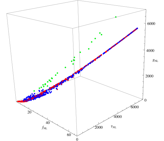
The non-Gaussianity parameters for the model in Sec. 3.2.1 are showed in Fig. 5.

Refer to caption
Figure 5: The non-Gaussianity parameters in the axion N-flation where Nfsubscript𝑁𝑓N_{f} inflatons have the same decay constant f𝑓f, and the decay constant of another inflaton is f¯¯𝑓\bar{f}. Here we consider the case with NNtot60similar-to-or-equalssubscript𝑁subscript𝑁𝑡𝑜𝑡similar-to-or-equals60N_{*}\simeq N_{tot}\simeq 60 and adopt f=1/2𝑓12f=1/2 and (πα¯ini)/π=2×104𝜋subscript¯𝛼𝑖𝑛𝑖𝜋2superscript104(\pi-{\bar{\alpha}}_{ini})/\pi=2\times 10^{-4}. The blue and green dots correspond to f¯=1/4¯𝑓14{\bar{f}}=1/4 and the red dots corresponds to f¯=1¯𝑓1{\bar{f}}=1. The green dots illustrate the case with detectable scale dependence of fNLsubscript𝑓𝑁𝐿f_{NL}.

Fitting the green dots corresponding to a detectable scale dependence of fNLsubscript𝑓𝑁𝐿f_{NL}, we find

τNL7.78fNL1.77,gNL2527τNL.formulae-sequencesimilar-to-or-equalssubscript𝜏𝑁𝐿7.78superscriptsubscript𝑓𝑁𝐿1.77similar-to-or-equalssubscript𝑔𝑁𝐿2527subscript𝜏𝑁𝐿\displaystyle\tau_{NL}\simeq 7.78f_{NL}^{1.77},\quad g_{NL}\simeq{25\over 27}\tau_{NL}. (87)

Fitting the blue and red dots respectively, we reach the same results

τNLsimilar-to-or-equalssubscript𝜏𝑁𝐿absent\displaystyle\tau_{NL}\simeq 8.28fNL1.59,gNL2527τNL.similar-to-or-equals8.28superscriptsubscript𝑓𝑁𝐿1.59subscript𝑔𝑁𝐿2527subscript𝜏𝑁𝐿\displaystyle 8.28f_{NL}^{1.59},\quad g_{NL}\simeq{25\over 27}\tau_{NL}. (88)

Here the relations between τNLsubscript𝜏𝑁𝐿\tau_{NL} and fNLsubscript𝑓𝑁𝐿f_{NL} depend on the choice of the parameters, such as f𝑓f, f¯¯𝑓\bar{f} and α¯¯𝛼\bar{\alpha}, in the model.

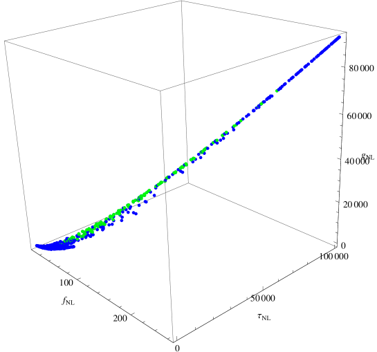
Similarly we also investigate the non-Gaussianity parameters for the model in Sec. 3.2.2. See the numerical results in Fig. 6.
Refer to caption
Figure 6: The non-Gaussianity parameters in the general axion N-flation with two kinds of inflatons. Here we consider the case with NNtot60similar-to-or-equalssubscript𝑁subscript𝑁𝑡𝑜𝑡similar-to-or-equals60N_{*}\simeq N_{tot}\simeq 60. The green dots illustrate the case with detectable scale dependence of fNLsubscript𝑓𝑁𝐿f_{NL}.

Fitting the blue and green dots respectively, we find

τNL7.16fNL1.72,gNL2527τNL.formulae-sequencesimilar-to-or-equalssubscript𝜏𝑁𝐿7.16superscriptsubscript𝑓𝑁𝐿1.72similar-to-or-equalssubscript𝑔𝑁𝐿2527subscript𝜏𝑁𝐿\displaystyle\tau_{NL}\simeq 7.16f_{NL}^{1.72},\quad g_{NL}\simeq{25\over 27}\tau_{NL}. (89)

To summarize, there is a universal relation between gNLsubscript𝑔𝑁𝐿g_{NL} and τNLsubscript𝜏𝑁𝐿\tau_{NL}, namely gNL2527τNLsimilar-to-or-equalssubscript𝑔𝑁𝐿2527subscript𝜏𝑁𝐿g_{NL}\simeq{25\over 27}\tau_{NL}. The value of gNLsubscript𝑔𝑁𝐿g_{NL} is the same order of τNLsubscript𝜏𝑁𝐿\tau_{NL}. But the relations between τNLsubscript𝜏𝑁𝐿\tau_{NL} and fNLsubscript𝑓𝑁𝐿f_{NL} are different for different cases.

References

  • [1] J. M. Maldacena, “Non-Gaussian features of primordial fluctuations in single field inflationary models,” JHEP 0305, 013 (2003) [arXiv:astro-ph/0210603].
  • [2] A. A. Starobinsky, “Multicomponent de Sitter (Inflationary) Stages and the Generation of Perturbations,” JETP Lett.  42 (1985) 152;
    M. Sasaki and E. D. Stewart, “A General Analytic Formula For The Spectral Index Of The Density Perturbations Produced During Inflation,” Prog. Theor. Phys.  95, 71 (1996) [arXiv:astro-ph/9507001];
    M. Sasaki and T. Tanaka, “Super-horizon scale dynamics of multi-scalar inflation,” Prog. Theor. Phys.  99, 763 (1998) [arXiv:gr-qc/9801017];
    D. H. Lyth, K. A. Malik and M. Sasaki, “A general proof of the conservation of the curvature perturbation,” JCAP 0505, 004 (2005) [arXiv:astro-ph/0411220];
    D. H. Lyth and Y. Rodriguez, “The inflationary prediction for primordial non-gaussianity,” Phys. Rev. Lett.  95, 121302 (2005) [arXiv:astro-ph/0504045].
  • [3] C. T. Byrnes, K. Y. Choi and L. M. H. Hall, “Conditions for large non-Gaussianity in two-field slow-roll inflation,” JCAP 0810, 008 (2008) [arXiv:0807.1101 [astro-ph]].
  • [4] C. T. Byrnes, K. Y. Choi and L. M. H. Hall, “Large non-Gaussianity from two-component hybrid inflation,” JCAP 0902, 017 (2009) [arXiv:0812.0807 [astro-ph]].
  • [5] S. A. Kim, A. R. Liddle and D. Seery, “Non-gaussianity in axion Nflation models,” arXiv:1005.4410 [astro-ph.CO].
  • [6] D. H. Lyth, “Generating the curvature perturbation at the end of inflation,” JCAP 0511, 006 (2005) [arXiv:astro-ph/0510443].
  • [7] M. Sasaki, “Multi-brid inflation and non-Gaussianity,” Prog. Theor. Phys.  120, 159 (2008) [arXiv:0805.0974 [astro-ph]].
  • [8] Q. G. Huang, “A geometric description of the non-Gaussianity generated at the end of multi-field inflation,” JCAP 0906, 035 (2009) [arXiv:0904.2649 [hep-th]].
  • [9] F. Vernizzi and D. Wands, “Non-Gaussianities in two-field inflation,” JCAP 0605, 019 (2006) [arXiv:astro-ph/0603799].
  • [10] S. A. Kim and A. R. Liddle, “Nflation: Multi-field inflationary dynamics and perturbations,” Phys. Rev.  D 74, 023513 (2006) [arXiv:astro-ph/0605604].
  • [11] Y. S. Piao, “On perturbation spectra of N-flation,” Phys. Rev.  D 74, 047302 (2006) [arXiv:gr-qc/0606034];
    R. G. Cai, B. Hu and Y. S. Piao, “Entropy Perturbations in N-flation Model,” Phys. Rev. D 80, 123505 (2009) [arXiv:0909.5251 [astro-ph.CO]].
  • [12] S. A. Kim and A. R. Liddle, “Nflation: Non-gaussianity in the horizon-crossing approximation,” Phys. Rev.  D 74, 063522 (2006) [arXiv:astro-ph/0608186].
  • [13] T. Battefeld and R. Easther, “Non-gaussianities in multi-field inflation,” JCAP 0703, 020 (2007) [arXiv:astro-ph/0610296].
  • [14] D. Battefeld and T. Battefeld, “Non-Gaussianities in N-flation,” JCAP 0705, 012 (2007) [arXiv:hep-th/0703012].
  • [15] D. Langlois, F. Vernizzi and D. Wands, “Non-linear isocurvature perturbations and non-Gaussianities,” JCAP 0812, 004 (2008) [arXiv:0809.4646 [astro-ph]].
  • [16] D. J. Mulryne, D. Seery and D. Wesley, “Moment transport equations for the primordial curvature perturbation,” arXiv:1008.3159 [astro-ph.CO].
  • [17] T. Wang, “Note on Non-Gaussianities in Two-field Inflation,” arXiv:1008.3198 [astro-ph.CO].
  • [18] T. Suyama, T. Takahashi, M. Yamaguchi and S. Yokoyama, “On Classification of Models of Large Local-Type Non-Gaussianity,” arXiv:1009.1979 [astro-ph.CO].
  • [19] E. Sefusatti, M. Liguori, A. P. S. Yadav, M. G. Jackson and E. Pajer, “Constraining Running Non-Gaussianity,” JCAP 0912, 022 (2009) [arXiv:0906.0232 [astro-ph.CO]].
  • [20] C. T. Byrnes, S. Nurmi, G. Tasinato and D. Wands, “Scale dependence of local fNLsubscript𝑓𝑁𝐿f_{NL},” JCAP 1002, 034 (2010) [arXiv:0911.2780 [astro-ph.CO]].
  • [21] C. T. Byrnes, M. Gerstenlauer, S. Nurmi, G. Tasinato and D. Wands, “Scale-dependent non-Gaussianity probes inflationary physics,” arXiv:1007.4277 [astro-ph.CO].
  • [22] C. T. Byrnes, K. Enqvist and T. Takahashi, “Scale-dependence of Non-Gaussianity in the Curvaton Model,” arXiv:1007.5148 [astro-ph.CO].
  • [23] Q. G. Huang, “Negative spectral index of fNLsubscript𝑓𝑁𝐿f_{NL} in the axion-type curvaton model,” arXiv:1008.2641 [astro-ph.CO].
  • [24] A. Riotto and M. S. Sloth, “Strongly Scale-dependent Non-Gaussianity,” arXiv:1009.3020 [astro-ph.CO].
  • [25] D. H. Lyth and A. Riotto, “Particle physics models of inflation and the cosmological density perturbation,” Phys. Rept.  314, 1 (1999) [arXiv:hep-ph/9807278].
  • [26] M. Sasaki and E. D. Stewart, “A General Analytic Formula For The Spectral Index Of The Density Perturbations Produced During Inflation,” Prog. Theor. Phys.  95, 71 (1996) [arXiv:astro-ph/9507001].
  • [27] E. Komatsu et al., “Seven-Year Wilkinson Microwave Anisotropy Probe (WMAP) Observations: Cosmological Interpretation,” arXiv:1001.4538 [astro-ph.CO].
  • [28] N. Arkani-Hamed, H. C. Cheng, P. Creminelli and L. Randall, “Extranatural inflation,” Phys. Rev. Lett.  90, 221302 (2003) [arXiv:hep-th/0301218].
  • [29] T. Banks, M. Dine, P. J. Fox and E. Gorbatov, “On the possibility of large axion decay constants,” JCAP 0306, 001 (2003) [arXiv:hep-th/0303252].
  • [30] S. Dimopoulos, S. Kachru, J. McGreevy and J. G. Wacker, “N-flation,” JCAP 0808, 003 (2008) [arXiv:hep-th/0507205].
  • [31] Q. G. Huang, “Weak Gravity Conjecture for the Effective Field Theories with N Species,” Phys. Rev.  D 77, 105029 (2008) [arXiv:0712.2859 [hep-th]].