Quantum chaos of a mixed, open system of kicked cold atoms

Abstract

The quantum and classical dynamics of particles kicked by a gaussian attractive potential are studied. Classically, it is an open mixed system (the motion in some parts of the phase space is chaotic, and in some parts it is regular). The fidelity (Loschmidt echo) is found to exhibit oscillations that can be determined from classical considerations but are sensitive to phase space structures that are smaller than Planck’s constant. Families of quasi-energies are determined from classical phase space structures. Substantial differences between the classical and quantum dynamics are found for time dependent scattering. It is argued that the system can be experimentally realized by cold atoms kicked by a gaussian light beam.

I Introduction

The quantum behavior of classically chaotic systems has been extensively studied both with time dependent and time independent Hamiltonians Tabor1989 ; OzoriodeAlmeida1988 ; Varenna1991 ; Gutzwiller1990 ; Oppo1994 ; Haake2001 ; Ott2002 . The main issue is that of determining fingerprints of classical chaos in the quantum mechanical behavior. For example, the spectral statistics of closed classically integrable Berry1976 ; Berry1977a ; Berry1977b and classically chaotic Bohigas1984 ; Sieber2001 ; MullerHaake2004 quantum systems have been predicted to have clearly distinct properties. Many of the systems that are of physical interest are mixed, where some parts of the phase space are chaotic and some parts are regular. Spectral properties of mixed systems with time independent Hamiltonians were studied by Berry and Robnik Berry1984 . In the present paper we study the classical/quantum correspondence properties of a mixed, open, time dependent system. (Here by “open” we mean that both position and momentum are unbounded.)

The system we study consists of a particle kicked by a Gaussian potential defined by the Hamiltonian,

$$H=\frac{p^{2}}{2m}-K^{\prime}Te^{-\frac{x^{2}}{2\Delta^{2}}}\sum_{n=-\infty}^{\infty}\delta\left(t-Tn\right).$$ (1)

Models of this form were studied by Jensen who used it to investigate quantum effects on scattering in classically chaotic Jensen1994 and mixed Jensen1992 systems. This system can be experimentally approximated by a Gaussian laser beam acting on a cloud of cold atoms, somewhat similar to the realization of the kicked rotor by Raizen and coworkers MooreRaizen1995 . As we will show, the study of Hamiltonian (1) is particularly suited to the investigation of generic behavior of kicked, open, mixed-phase-space systems. In particular, we will focus on issues of fidelity Peres1984 ; Jalabert2001 ; Jacquod2002 ; Gorin2006 , decoherence HansonOtt1984a ; Cohen1991 and scattering Blummel1988 ; Jalabert1990 ; Doron1991 ; Lai1992 . Our main motivation in studying Hamiltonian (1) is that, with likely future technological advances (see Sec. VII for discussion), the phenomena we consider may soon become accessible to experimental investigation.

Quantum mechanically, it is expected that classical phase space details on the scale of Planck’s constant are washed out Berry1972 ; Berry1977c . In contrast, one of our results will be that quantum dynamics can be sensitive to extremely fine structures in phase space, and this sensitivity is stable in the presence of noise HansonOtt1984a ; Cohen1991 . Phase space tunneling has been studied extensively Hanson1984 ; Tomsovic1994 ; Sheinman2006 ; Lock2010 . For systems with many phase space structures complications arise due to transport between these structures. For our Hamiltonian (1) the motion is unbounded (i.e., the system is “open”), and therefore this system is ideal for the exploration of tunneling out of phase space structures and, in particular, for study of resonance assisted tunneling, a current active field of research Tomsovic1994 ; Sheinman2006 ; Lock2010 .

The outline of our paper is as follows. Section II presents and discusses our model system. Section III considers the quasi-energies of quantum states localized to island chains. Section IV introduces the fidelity concept and applies it to study different regions of the phase space including the main, central KAM island (Sec. IV.1), island chains (Sec. IV.2), and chaotic regions (Sec. IV.3). Experimentally there is always some noise present in such systems. Also, noise can be intentionally introduced. Section V considers this issue. Section VI presents a study of the scattering properties of the system. Conclusions and further discussion are given in Sec. VII.

II The model

II.1 Formulation

A particle kicked by a Gaussian beam is modeled by the Hamiltonian, Eq. (1), with the classical equations of motion,

$$\dot{p} = -\frac{\partial H}{\partial x}=-K^{\prime}T\frac{x}{\Delta^{2}}e^{-\frac{x^{2}}{2\Delta^{2}}}\sum_{n=-\infty}^{\infty}\delta\left(t-Tn\right),$$ (2)

$$\dot{x} = \frac{\partial H}{\partial p}=\frac{p}{m}.$$

We rewrite the equations of motion in dimensionless form by defining $\bar{x}=x/\Delta$, $\bar{t}=t/T$. The dimensionless momentum is correspondingly defined as $\bar{p}=pT/\left(m\Delta\right)$. Thus we obtain the dimensionless equations of motion,

$$\dot{\bar{p}} = -K\bar{x}e^{-\frac{\bar{x}^{2}}{2}}\sum_{n=-\infty}^{\infty}\delta\left(\bar{t}-n\right),$$ (3)

$$\dot{\bar{x}} = \bar{p},$$

where

$$K=\frac{K^{\prime}T^{2}}{m\Delta^{2}}.$$ (4)

Since in what follows we deal with the rescaled position, momentum and time we will drop the bar notation for convenience. By integrating (2) and defining $p_{n}=p\left(t=n_{-}\right)$, $x_{n}=x\left(t=n_{-}\right)$, where $t=n_{-}$ is a time just before the n-th kick, we can rewrite the differential equations of the motion as a mapping, $M$,

$$M:\qquad\begin{cases}p_{n+1}&=p_{n}-Kx_{n}e^{-\frac{x_{n}^{2}}{2}},\\ x_{n+1}&=x_{n}+p_{n+1}.\end{cases}$$ (5)

The corresponding quantum dynamics in rescaled units is given by the Hamiltonian,

$$H=\frac{p^{2}}{2}-Ke^{-\frac{x^{2}}{2}}\sum_{n=-\infty}^{\infty}\delta\left(t-n\right),$$ (6)

where $p=-i\tau\partial_{x}$, and $\tau=\hbar T/\left(m\Delta^{2}\right)$ is the rescaled $\hbar$, namely, $\left[x,p\right]=i\tau$. The quantum evolution is given by

$$i\tau\partial_{t}\psi=-\frac{\tau^{2}}{2}\partial_{xx}\psi-Ke^{-\frac{x^{2}}{2}}\sum_{n=-\infty}^{\infty}\delta\left(t-n\right)\psi,$$ (7)

or by the one kick propagator

$$U_{1}=e^{-i\frac{p^{2}}{2\tau}}\exp\left(i\frac{K}{\tau}e^{-\frac{x^{2}}{2}}\right).$$ (8)

II.2 Properties of the Classical Map and the phase portrait

In this subsection the classical properties of the map Eq. (5) will be presented. The first property is reflection symmetry, $\left(x,p\right)\rightarrow\left(-x,-p\right)$. Phase portraits such as these presented in Fig. 1 and Fig. 2

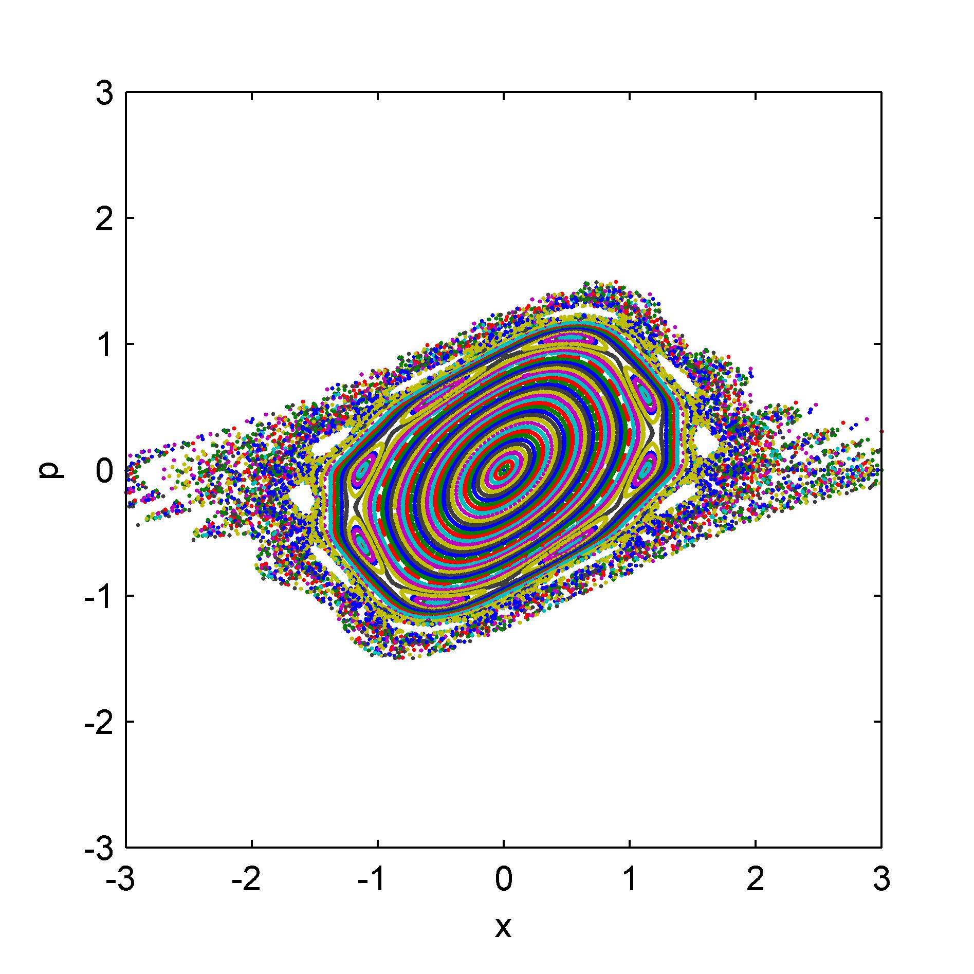
Figure 1: (Color online) The phase space for $K=1$. Colors (shades) distinguish different orbits.

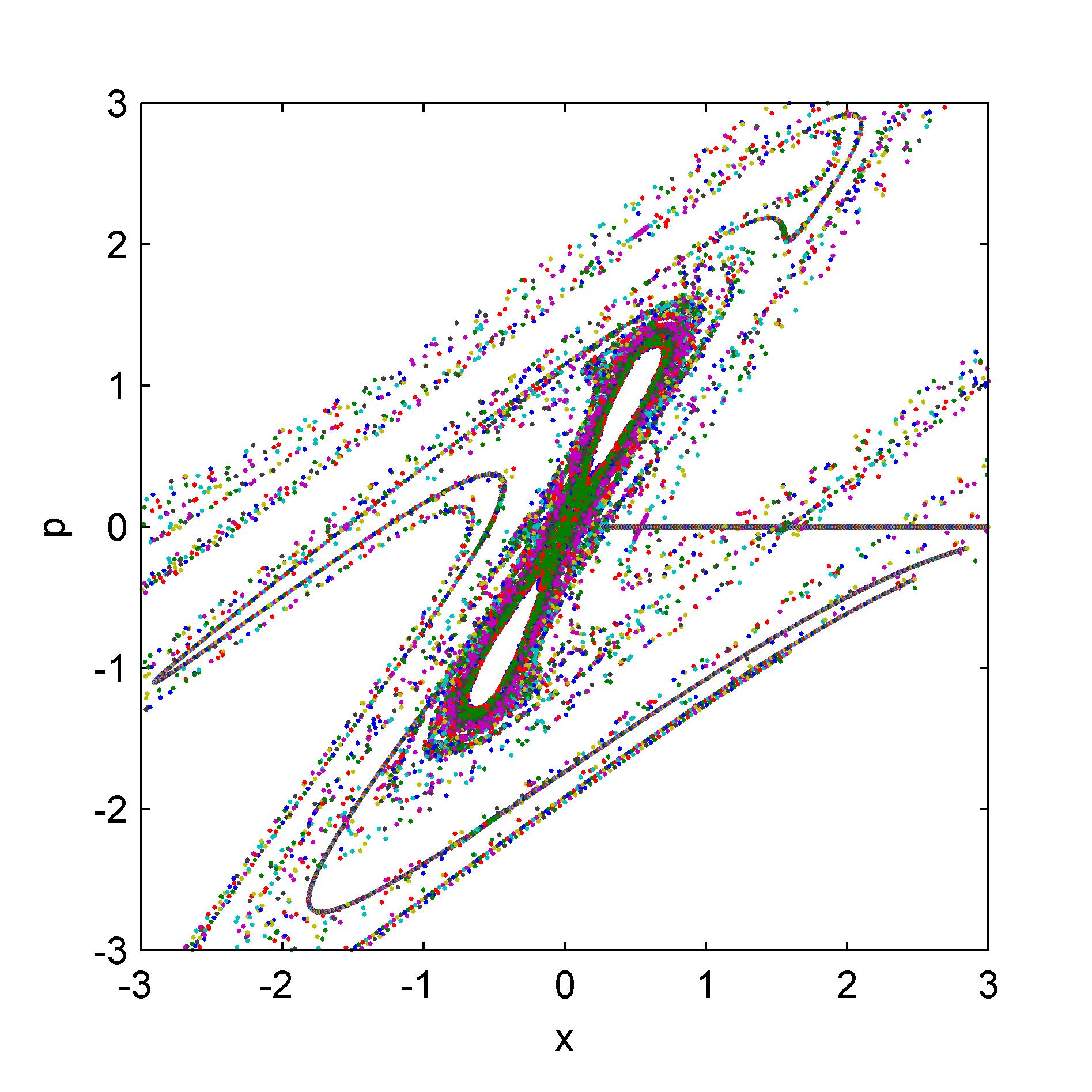
Figure 2: (Color online) The phase space for $K=4.5$. Colors (shades) distinguish different orbits.

are clearly seen to satisfy this property. Like the standard map, Eq. (5) can be written as a product of two involutions, $M=J_{2}J_{1}$, where

$$J_{1}:\qquad\left(p,x\right) \rightarrow \left(-p,x+p\right)$$ (9)

$$J_{2}:\qquad\left(p,x\right) \rightarrow \left(-p-Kxe^{-\frac{x^{2}}{2}},x\right).$$

We will use this property for the calculation of the periodic orbits. From (5) we see that the only fixed point is $\left(x=0,p=0\right)$. Linearizing around this point, we find that the trace of the tangent map is $2-K$. Therefore, this point is elliptic for $0<K<4$, and, for $K=1$, the phase portrait of Fig. 1 is found, while for $K>4$ this point is hyperbolic, leading to phase portraits like that of Fig. 2. Since the kicking as a function of $x$ is bounded by $K$, for large initial momentum the particle is nearly not affected by the kicks, and continues to move in its initial direction. For $0<K<4$ we find a large island around the elliptic point $\left(x,p\right)=\mbox{$\left(0,0\right)$}$, and, for nearly all initial conditions near $x=p=0$, the motion is regular (i.e., lies on KAM surfaces). Further away from this fixed point, one finds island chains embedded in a chaotic strip. And even further away, the motion is unbounded.

III Quasi-energies of an island chain

In the semiclassical regime quasi-energies are related to classical structures. In this section we assume the existence of quasi-energy eigenfunctions $u_{n}\left(x\right)$,

$$U_{1}u_{n}\left(x\right)=e^{-iE_{n}}u_{n}\left(x\right),$$ (10)

such that $u_{n}\left(x\right)$ is strongly localized to an island chain of order $r$, and we attempt to calculate the quasi-energy $E_{n}$. For this purpose we use the one-kick propagator $U_{1}$ to generate successive jumps in the island chain,

$$U_{1}\psi_{i}=\psi_{i+1},$$ (11)

where $\psi_{i}$ is a wavefunction which is localized in island number $i$ within the island chain. Further, we assume that this wavefunction can be expanded using the quasi-eigenstates of the island chain,

$$\psi_{i}=\sum_{n}c_{in}u_{n}\left(x\right).$$ (12)

Using this expansion we obtain a system of equations,

$$U_{1}\psi_{i}=\sum_{n}c_{in}u_{n}\left(x\right)e^{-iE_{n}},$$ (13)

and

$$U_{1}^{r}\psi_{i}=\sum_{n}c_{in}u_{n}\left(x\right)e^{-iE_{n}r}.$$ (14)

Classically the $i-$th island is transformed to itself by $r$ successive applications of the map $M$. In particular, an elliptic fixed point of the map $M^{r}$ is located in the center of the island. In the semiclassical limit the eigenstates of $U_{1}^{r}$ are determined by $M^{r}$ and are close to the eigenstates of a harmonic oscillator centered on the fixed point of $M^{r}$. The frequency of the oscillator, $\nu_{i}$, is such that the eigenvalues of the tangent map of $M^{r}$, which transforms the $i-$th island to itself, are $e^{\pm i\nu_{i}}$. This tangent map can be written in terms of the product of the tangent maps of $M\left(i\rightarrow i+1\right),$ which transform the $i-$th island to the $\left(i+1\right)-$th island. Consequently, since the eigenvalues are determined by the trace of the product of the tangent maps, they are independent of $i$ (due to the invariance of the trace to cyclic permutations). In what follows we therefore drop the index $i$ from $\nu_{i}$.

Choosing $\psi_{i}$ as the eigenstate of $U_{1}^{r}$, means that

$$U_{1}^{r}\psi_{i}=e^{i\bar{\beta}}\psi_{i},$$ (15)

where $\bar{\beta}=\tau\nu/2$ and we have taken $\psi_{i}$ to be the ground state of the harmonic oscillator. Therefore,

$$\psi_{i}=\sum_{n}c_{in}u_{n}\left(x\right)e^{-i\left(E_{n}r+\bar{\beta}\right)}.$$ (16)

Using the orthogonality of the $u_{n}\left(x\right)$, Eqs. (16) and (12) yield

$$e^{-i\left(E_{n}r+\bar{\beta}\right)}=1.$$ (17)

The quasi-energies, obtained from (17) are, therefore,

$$E_{n}=\frac{2\pi}{r}n+\beta,\qquad 0\leq n\leq r,$$ (18)

where $\beta=-\bar{\beta}/r$. Approximations to the quasi-energies can be calculated numerically by launching a wavepacket into one island in the island chain and propagating it in time, which gives

$$\psi\left(x,N\right)=\sum_{n}c_{in}u_{n}\left(x\right)e^{-iE_{n}N}.$$ (19)

Taking a Fourier transform with respect to $N$ gives the quasi-energies. We have found that for $K=1$ the chains with $r=8$ and $r=16$ accurately satisfy (18).

IV Fidelity

The concept of quantum fidelity was introduced by Peres Peres1984 as a fingerprint of classical chaos in quantum dynamics. It has subsequently been extensively utilized in theoretical Jalabert2001 ; Jacquod2002 ; Cerruti2002 ; Wimberger2006 and experimental studies Andersen2004 ; Kaplan2005 ; Wimberger2006 ; Andersen2006 , for a review see Gorin2006 . Most of this research has focused on the difference between chaotic and regular systems. Here we discuss fidelity for a mixed system. We have calculated the fidelity,

$$S\left(t\right)=\left|\left\langle\phi_{0}\right|e^{iH_{1}t/\tau}e^{-iH_{2}t/\tau}\left|\phi_{0}\right\rangle\right|^{2},$$ (20)

where $H_{1,2}$ are Hamiltonians of the form (6) with with slightly different kicking strengths, $K_{1,2}$, and $\phi_{0}$ is the initial wavefunction. We note that the fidelity $S\left(t\right)$ can be experimentally measured by the Ramsey method, as used in Ref. Kaplan2005 . The fidelity is related to an integral over Wigner functions,

$$S\left(t\right)=2\pi\tau\int dxdp\,P_{\phi_{1}}\left(x,p\right)P_{\phi_{2}}\left(x,p\right),$$ (21)

where $P_{\phi_{1,2}}$ are the Wigner functions of $\phi_{1,2}=e^{-iH_{1,2}t/\tau}\phi_{0}$, respectively.

We study separately the fidelity in the central island, in the island chain, and in the chaotic region (i.e., Eq.(20) with $\phi_{0}$ localized to these regions).

IV.1 Fidelity of a wavepacket in the central island

First we prepare the initial wavefunction $\phi_{0}$ as a Gaussian wavepacket with a minimal uncertainty, namely, $\Delta x=\Delta p=\left(\tau/2\right)^{\nicefrac{{1}}{{2}}}$,

$$\phi_{0}\left(x\right)=\frac{1}{\left(2\pi\left(\Delta x\right)^{2}\right)^{\nicefrac{{1}}{{4}}}}e^{-ip_{0}x/\tau}\exp\left[-\frac{\left(x-x_{0}\right)^{2}}{4\left(\Delta x\right)^{2}}\right].$$ (22)

We place $\phi_{0}$ in the center of the island, namely, $x_{0}=p_{0}=0$. Since the center of the wavepacket is initially at the fixed point, for $\Delta x$ and $\Delta p$ classically small, its dynamics are approximately determined by the tangent map of the fixed point. For this purpose we linearize the classical map (5) around the point $x=p=0$. This gives the equation for the deviations,

$$\left(\begin{array}[]{c}\delta x_{n+1}\\ \delta p_{n+1}\end{array}\right)=\left(\begin{array}[]{cc}\left(1-K\right)&1\\ -K&1\end{array}\right)\left(\begin{array}[]{c}\delta x_{n}\\ \delta p_{n}\end{array}\right).$$ (23)

The eigenvalues of this equation are,

$$\alpha_{1,2}=\frac{\left(2-K\right)}{2}\pm\frac{i\sqrt{K\left(4-K\right)}}{2}\equiv e^{\pm i\omega},$$ (24)

with

$$\omega=\arctan\frac{\sqrt{K\left(4-K\right)}}{\left(2-K\right)},$$ (25)

which is the angular velocity of the points around the origin. In the vicinity of the fixed point, the system behaves like a harmonic oscillator with a frequency $\omega$. Classically, the motion of the trajectories, starting near the elliptic fixed point, $x=p=0$, stays there because the region is bounded by KAM curves that surround this point. For small effective Planck’s constant, $\tau$, the quantum behavior is expected to mimic the classical behavior for a long time. Inspired by the relation between the fidelity and the Wigner function (see (21)), we have defined a classical fidelity, $S_{c}\left(t\right)$, as the overlap between coarse-grained Liouville densities of $H_{1}$ and $H_{2}$ (this is similar to the classical fidelity defined in Nielsen2000 ). To do this we first randomly generate a large number of initial classical positions using the initial distribution function,

$$f_{0}\left(x,p\right)=\frac{1}{2\pi\Delta x\Delta p}\exp\left\{-\frac{1}{2}\left[\left(\frac{x-x_{0}}{\Delta x}\right)^{2}+\left(\frac{p-p_{0}}{\Delta p}\right)^{2}\right]\right\},$$ (26)

corresponding to our initial $\phi_{0}$ given by (22). The coarse grained densities for $H_{1}$ and $H_{2}$ are then computed by first integrating these initial conditions and then coarse graining to a grid of squares in phase space of area $\tau$ Berry1979 . The motivation for this procedure is to check if structures in phase space of size smaller than $\tau$ are of importance to the fidelity. A comparison between $S\left(t\right)$ and $S_{c}\left(t\right)$ for $x_{0}=-0.25$, $p_{0}=0$, and $\tau=0.01$ is presented in Fig. 3.

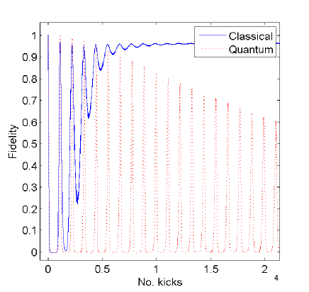
Figure 3: (Color online) Quantum fidelity, $S\left(t\right)$, (dashed red) and classical fidelity, $S_{c}\left(t\right)$ (solid blue). $K_{1}=1$, $K_{2}=1.01$, $\tau=0.01$, $x_{0}=-0.25$ and $p_{0}=0$.

The initial wavepacket is smeared on a ring in the phase space due to the twist property of the map. Since the probability density is preserved, the “whorl” which is formed contains very dense and thin tendrils. In Fig. 4

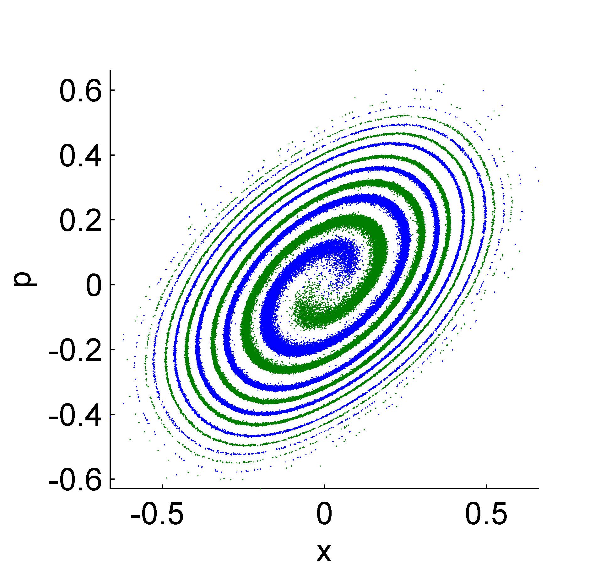
Figure 4: (Color online) Classical density, which was initially placed at $x_{0}=-0.25$ and $p_{0}=0$ after $500$ kicks. Blue (dark) dots are for $K_{1}=1$ and green (light) dots are for $K_{2}=1.01$.

two such “whorls” are presented for $H_{1}$ with $K_{1}=1$ and $H_{2}$ with $K_{2}=1.01$. When the two “whorls” coincide a fidelity revival is formed. Coarse graining the densities to a boxes of size $\tau$ averages the differences between the two “whorls”, obtained by $H_{1}$ and $H_{2}$. This explains why the classical fidelity approaches $1$ as the number of kicks becomes large. On the other hand, the quantum fidelity shows strong revivals which suggests that it feels the difference in trajectories between the two Hamiltonians. To understand the period of the revivals, we calculate, $\delta\omega$, the frequency difference between the two Hamiltonians, $H_{1,2}$. Expanding $\omega$ around $K_{1}$ gives

$$\omega\left(K\right)=\omega\left(K_{1}\right)+\frac{K-K_{1}}{\sqrt{K\left(4-K\right)}}+O\left(\left(K-K_{1}\right)^{2}\right).$$ (27)

Therefore, the difference in angular velocity between two orbits of Hamiltonians, $H_{1}$ and $H_{2}$ is given by

$$\delta\omega=\omega\left(K_{2}\right)-\omega\left(K_{1}\right)=\frac{\delta K}{\sqrt{K_{2}\left(4-K_{2}\right)}},$$ (28)

for $\delta K=K_{2}-K_{1}$. This suggests that the fidelity, $S\left(t\right)$ will be periodic, with the period $T=\pi/\delta\omega$. Note that we predict $T=\pi/\delta\omega$, rather than $T=2\pi/\delta\omega$. This is because of the symmetry of the initial condition. Each point of $H_{1}$ is chasing a point of $H_{2}$ which is its reflection through the origin of the phase space and, therefore, is found first at an angle of $\pi$ and not $2\pi$. To check this, we have calculated the period of the revivals numerically for $0<K<4$. First, fidelity was computed and Fourier transformed, then the second most significant value was taken as the period. In Fig. 5 we present a comparison of the analytic calculation of the period of the fidelity and the numerical computation. The correspondence is good through the whole range of the stochasticity parameter $K$ but degrades near $K=4$, where the elliptic point at the origin becomes unstable. Also, near $K=2$, resonance chains appear near the fixed point $x=p=0$, which results in poor agreement with the theoretical prediction, see Fig. 7.

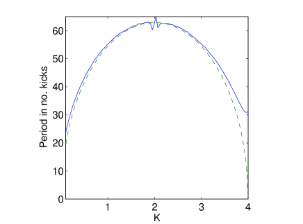
Figure 5: (Color online) A numerical (̇solid blue) and an analytical (dashed green) computation of the period of the fidelity revival as a function of $K$, $\delta K=0.1$, $x_{0}=p_{0}=0$, $\tau=0.01$.

Very often it is assumed that quantum mechanical behavior is insensitive to phase space structures with areas smaller than Planck’s constant, which results in an effective averaging on this scale Berry1972 ; Berry1977c . While this assumption is often correct Sheinman2006 , sometimes it is not HensingerPhillips2001 ; SteckRaizen2001 ; SteckRaizen2002 ; AverbukhMoiseyev1995 ; AverbukhMoiseyev2002 ; OsovskiMoiseyev2005 . The difference between $S\left(t\right)$ and $S_{c}\left(t\right)$ demonstrated in Fig. 3 shows that fidelity may be sensitive to extremely small details in the classical phase space. In particular, a “whorl” Berry1972 ; Berry1977c affects the quantum dynamics. The small decay of the quantum fidelity seen in Fig. 3 is a result of tunneling.

We stress that to observe the oscillations which appear on Fig. 3 requires sensitivity to the structure of the “whorl” of Fig. 4. In our quantum calculation the effective Planck’s constant is $\tau=0.01$ and it is obvious that the “whorl” of Fig. 4 exhibits structures on smaller scale, for example, in a square with sides of length $0.1$ in phase space (of Fig. 4) one finds several stripes of the “whorl”. Indeed, averaging over such a square leads to the classical fidelity that does not exhibit oscillations as the quantum fidelity does. We conclude that the structures on the scale smaller than the effective Planck’s constant, $\tau$, are crucial for the oscillations in the quantum fidelity. Hence, structures of scales smaller than Planck’s constant may dominate fidelity, which is a quantum quantity.

For a wavepacket started around an initial point $\left(x_{0},p_{0}\right)\neq\left(0,0\right)$ the behavior is similar, but with a slightly different period due to a decrease in the angular velocity for points far from the fixed point. Similarly to the case of $\left(x_{0},p_{0}\right)=\left(0,0\right)$, we have calculated numerically the revival period for different values of $K$; this is shown in Fig. 6

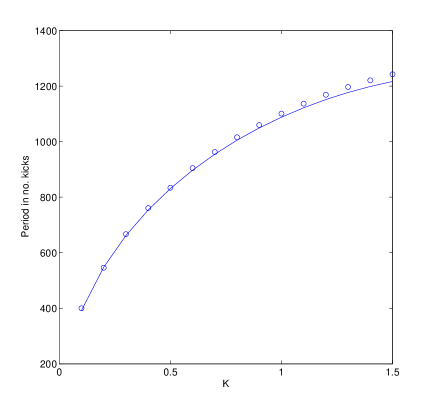
Figure 6: A numerical (blue circles) and an analytical (solid blue line) computation of the period of the fidelity revival as a function of $K$, $\delta K=0.01$, $x_{0}=-0.25$, $p_{0}=0$, $\tau=2\times 10^{-4}$.

. For $K>1.5$ resonances appear near the launching point which introduce additional periods into the fidelity, making the analysis more complicated.

IV.2 Fidelity for a wavepacket in an island chain

We consider two different island chains occurring for different values of $K$. For $K=2.1$ we have examined a chain of order $r=4$ (see Fig. 7)

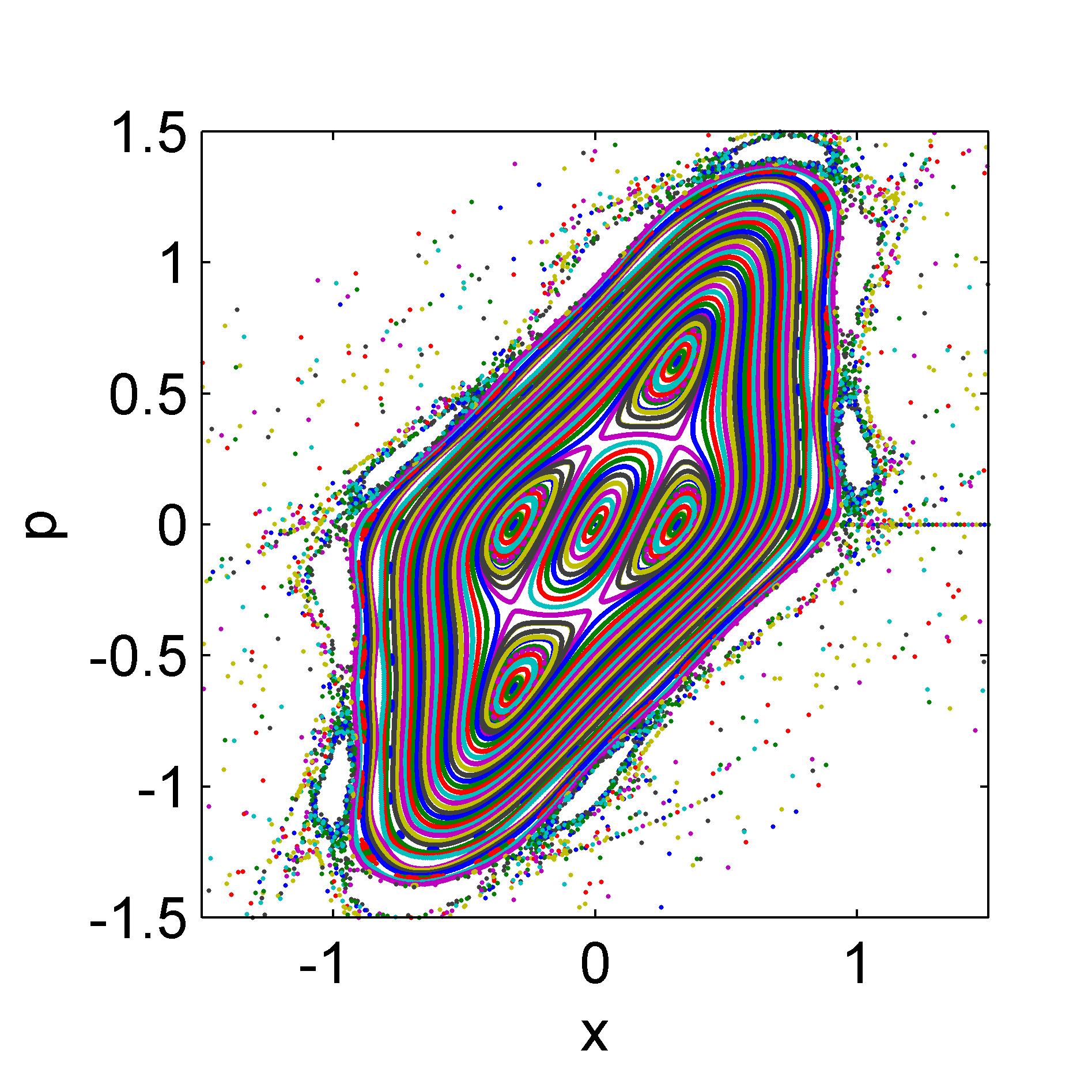
Figure 7: (Color online) The phase space for $K=2.1$. Colors (shades) distinguish different orbits.

, and for $K=1$ we have studied a chain of order $r=8$ (see Fig. 1). The initial wavepacket was launched inside one of the islands of the chain, and the we numerically computed the fidelity. In Figs. 8 ($K_{1}=2.10$, $K_{2}=2.11$) and 9 ($K_{1}=1.00$, $K_{2}=1.01$)

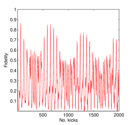
Figure 8: Fidelity of packet started inside an island chain of order $4$. $K_{1}=2.10$, $K_{2}=2.11$, $\tau=2\times 10^{-4}$, and the center of the packet is started at $x=0.3198$, $p=0$, in the center of one of the islands of the chain.

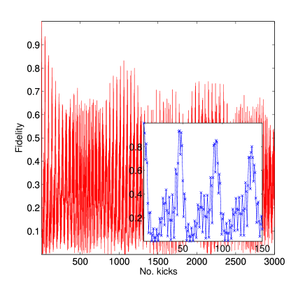
Figure 9: Fidelity of packet started inside an island chain of order $8$. $K_{1}=1$, $K_{2}=1.01$, $\tau=2\times 10^{-4}$, and the center of the packet is started at $x=1.1312$, $p=0$, in the center of one of the islands of the chain. The inset is a zoom on the graph.

we show the results of these computations.

It is notable that there are three timescales in the graph of the fidelity. The shortest timescale is visible only in the inset of Fig. 9 and may be understood taking into account the symmetry of the equations of motion, $x\rightarrow-x,$ $p\rightarrow-p$. This symmetry implies that each island has a “twin” which is found by reflection through the origin, $x=p=0$. Therefore, the overlap between the islands of $H_{1}$ and $H_{2}$ is a periodic function with a period of $\nicefrac{{r}}{{2}}$, where $r$ is the number of islands in the chain. Consequently, for the island chains used to obtain Fig. 8 and 9, the fidelity has periods of $2$ and $4$, respectively, on its shortest timescale. The intermediate timescale is due to a rotation of the wavepacket around the elliptic points of the island where it is initially launched. The central point in the island is a fixed point of $M^{r}$. In $r$ iterations, points in the island rotate with an angular velocity $\omega_{1}$ and $\omega_{2}$ for $H_{1}$ and $H_{2}$, respectively. The angular velocities can be calculated numerically by linearization of the tangent map of $M^{r}$ around the fixed point of the map $M^{r}$. We find the fixed point by reducing $M$ to a product of involutions (9), which allows us to reduce the search for the fixed points to the line $p=0$ in the phase space since any point on this line is a fixed point of $J_{1}$ Greene1979 ; Hihinashvili2007 . For $K_{1}=1$ and $K_{2}=1.01$, the angular velocities are found to be $\omega_{1}=1.10$ and $\omega_{2}=1.147$. For $K_{1}=2.10$ and $K_{2}=2.11$, the angular velocities are found to be $\omega_{1}=0.391$ and $\omega_{2}=0.429$. Therefore, the time it takes for a packet to accomplish a full revolution around the fixed points of $M^{r}$ is $2\pi r/\bar{\omega}$, where $\bar{\omega}=\frac{1}{2}\left(\omega_{1}+\omega_{2}\right)\approx\omega_{1}\approx\omega_{2}$ (see Table 1). The longest timescale of the fidelity is the timescale when the difference between the angular velocities is resolved $T=2\pi r/\delta\omega$. In Table 1 we compare those periods deduced directly from Fig. 8 and Fig. 9 and the periods calculated by finding $\omega_{1,2}$ from the tangent map. We see that the agreement is excellent.

	$r=4$		$r=8$
	Fig.8	Tangent map	Fig.9	Tangent map
shortest period	2	2	4	4
medium period	62	$61.3$	44	$44.7$
longest period	651	$657.8$	1061	$1077.4$

Table 1: This table compares two ways of calculating the periods of revivals for the resonance chains. In one way we have deduced them from the Figures 8,9, and in the other way we have calculated them using the tangent map. This is done for two different resonances: $r=4$, for $K_{1}=2.1$, $K_{2}=2.11$; and $r=8$ for $K_{1}=1$, $K_{2}=1.01$. For both cases $\tau=2\times 10^{-4}$.

IV.3 Fidelity of the wavepacket in the chaotic strip

For the fidelity of a packet started inside the chaotic strip (see Fig. 10), we notice a strong revival after 6 kicks which is dependent on $K_{1}$. This is half a period in this chain/strip. After this revival the fidelity decays to zero, which is a characteristic of chaotic regions.

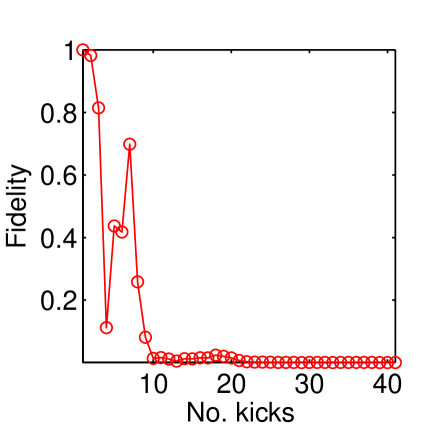
Figure 10: Fidelity of packet started inside a chaotic layer. $K_{1}=1$, $K_{2}=1.01$, $\tau=2\times 10^{-4}$ and the center of the packet is started at $x=-2$, $p=0$.

Detailed exploration of this region is left for further studies.

V Dephasing

We now investigate the effect of dephasing by adding temporal noise to the time between the kicks. The classical equations of motion with the dephasing are given by

$$p_{n+1} = p_{n}-Kx_{n}e^{-\frac{x_{n}^{2}}{2}},$$ (29)

$$x_{n+1} = x_{n}+\left(1+\delta t_{n}\right)\cdot p_{n+1},$$

and the quantum one kick propagator is

$$U_{1}=e^{-i\frac{p^{2}}{2\tau}\left(1+\delta t_{n}\right)}\exp\left(i\frac{K}{\tau}e^{-\frac{x^{2}}{2}}\right),$$ (30)

where $\delta t_{n}$ is a random variable which is normally distributed with zero mean and a standard deviation $\sigma_{t}$. The standard deviation of the $\delta t_{n}$, corresponds to the strength of the noise. We find that the noise results in an escape outside of the island, which yields additional decay in the fidelity. Since we are interested in the difference between the two wavefunctions only inside the main island, for each kick we normalize the wavefunctions of $H_{1}$ and $H_{2}$ such that their norm is equal to $1$ inside a region of $\left|x\right|\leq x_{b}=3$. This gives the following expression for the fidelity

$$S\left(t\right)=\frac{\int_{-x_{b}}^{x_{b}}\left(e^{-iH_{1}t/\tau}\phi_{0}\left(x^{\prime}\right)\right)\left(e^{-iH_{2}t/\tau}\phi_{0}\left(x^{\prime}\right)\right)\,dx^{\prime}}{\left(\int_{-x_{b}}^{x_{b}}\left|e^{-iH_{1}t/\tau}\phi_{0}\left(x^{\prime}\right)\right|^{2}dx^{\prime}\right)^{\nicefrac{{1}}{{2}}}\left(\int_{-x_{b}}^{x_{b}}\left|e^{-iH_{2}t/\tau}\phi_{0}\left(x^{\prime}\right)\right|^{2}dx^{\prime}\right)^{\nicefrac{{1}}{{2}}}},$$

with he classical fidelity $S_{c}\left(t\right)$ defined in a similar way. We have numerically calculated the fidelity for the same situation as in Fig. 3 with added relative noise of $\sigma_{t}=0.01$ (Fig. 11) and $\sigma_{t}=0.001$ (Fig. 12).

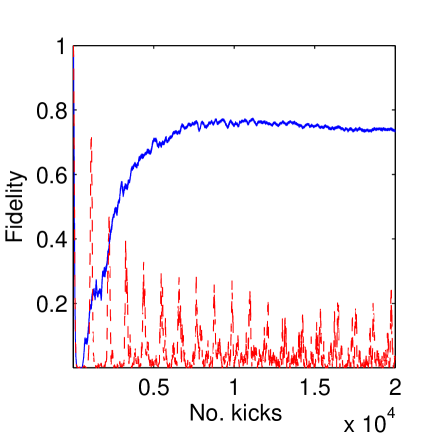
Figure 11: (Color online) Quantum fidelity, $S\left(t\right)$, (dashed red) and classical fidelity, $S_{c}\left(t\right)$ (solid blue) for a dephasing noise of strength $\sigma_{t}=0.01$, $K_{1}=1$, $K_{2}=1.01$, $\tau=0.01$, $x_{0}=-0.25$ and $p_{0}=0$.

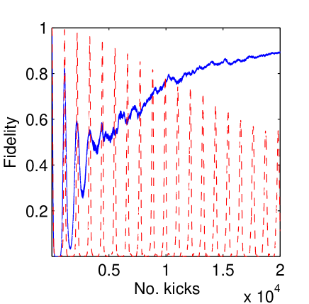
Figure 12: (Color online) Quantum fidelity, $S\left(t\right)$, (dashed red) and classical fidelity, $S_{c}\left(t\right)$ (solid blue) for a dephasing noise of strength $\sigma_{t}=0.001$, $K_{1}=1$, $K_{2}=1.01$, $\tau=0.01$, $x_{0}=-0.25$ and $p_{0}=0$.

We notice that the noise introduces additional decay in the quantum fidelity.

To isolate the effect of noise from the decay in the fidelity due to the difference between $K_{1}$ and $K_{2}$ we set $K_{1}=K_{2}$ and use two different noise realizations with the same strength $\sigma_{t}$. From Fig. 13

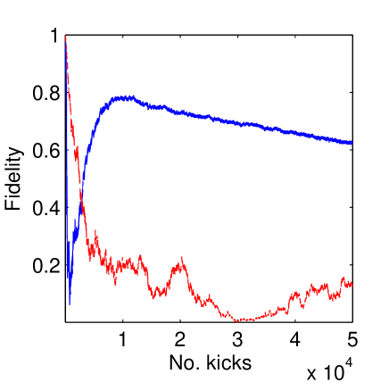
Figure 13: (Color online) Quantum fidelity, $S\left(t\right)$, (dashed light red) and classical fidelity, $S_{c}\left(t\right)$ (solid dark blue) for two different realizations of a dephasing noise of strength $\sigma_{t}=0.001$, $K_{1}=K_{2}=1$, $\tau=0.01$, $x_{0}=-0.25$ and $p_{0}=0$.

we notice that classical fidelity initially decays very fast due to the noise and than slowly recovers approaching a value of $0.8$. This is due to the coarse graining to the scale of $\tau$. To illustrate this we plot in Fig. 14

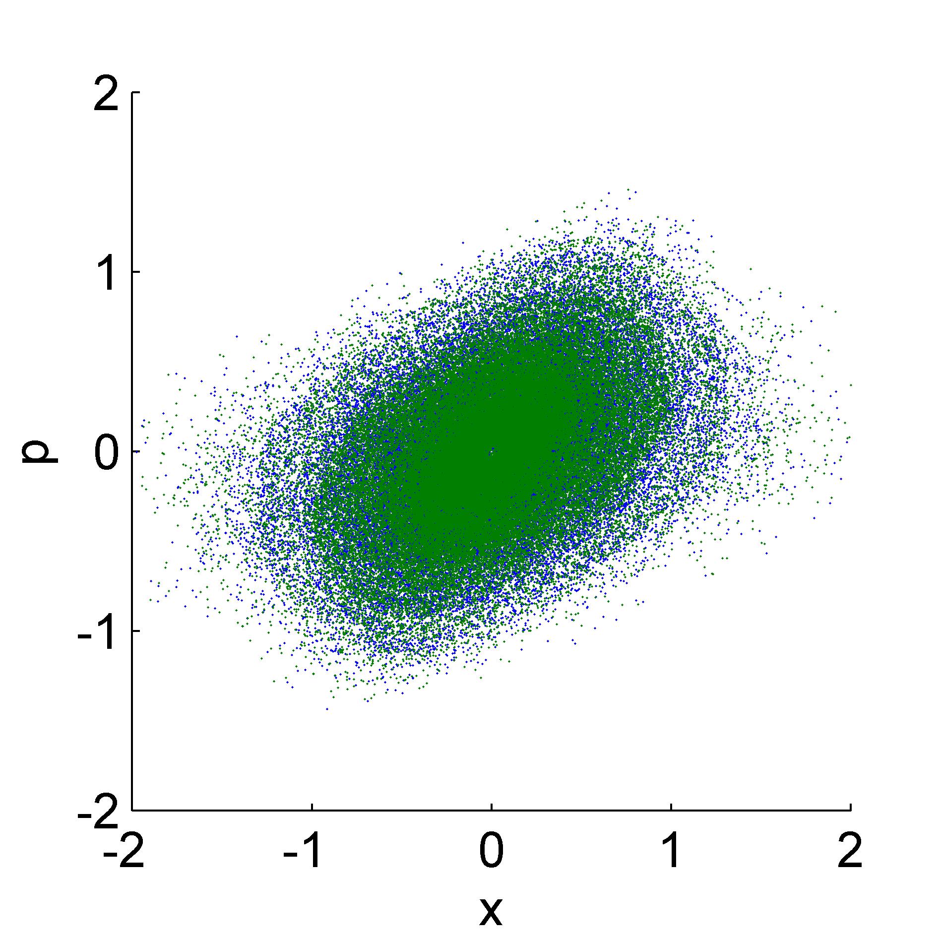
Figure 14: (Color online) Classical density, which was initially placed at $x_{0}=-0.25$ and $p_{0}=0$ after $5\times 10^{4}$ kicks, $K_{1}=K_{2}=1$. Colors (shades) correspond to two different realizations of a dephasing noise of strength $\sigma_{t}=0.01$.

the classical densities after $5\times 10^{4}$ kicks for a packet initially launched at $x_{0}=-0.25$. We notice that the densities for the two Hamiltonians highly overlap, which explains the high fidelity. In Fig. 15

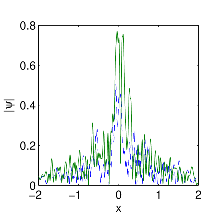
Figure 15: (Color online) Wavepackets, which were initially placed at $x_{0}=-0.25$ and $p_{0}=0$ after $5\times 10^{4}$ kicks, $K_{1}=K_{2}=1$. Colors (shades) correspond to two different realizations of a dephasing noise of strength $\sigma_{t}=0.01$.

we observe the corresponding quantum wavepackets. Contrary to the classical fidelity, the quantum fidelity decays rather slowly with the noise, suggesting that it is more robust to noise than the classical fidelity.

VI Scattering

We now investigate the difference between quantum and classical scattering behavior by studying the evolution of a wavepacket initialized outside of the main island of the phase space, Eq. (22) with $x_{0}=-2$, $p_{0}=0$, $\Delta x=\Delta p=\left(\tau/2\right)^{\nicefrac{{1}}{{2}}}$. In the classical case both the classical chaos, as well as the numerous small island structures introduce, an erratic behavior for the transmission and reflection coefficients as a function of the initial launching position and energy Jensen1992 ; Jensen1994 . Due to effective phase space smoothing of areas much smaller than our effective Planck’s constant, $\tau$, we expect that fine scale fractal-like features in the classically erratic scattering dependence will be averaged out. To quantify this behavior, we measure the transmission and reflection coefficients for a wavepacket defined as the transfered or reflected probability mass, either quantum or classical. Classically, it is the fraction of initial trajectories (generated using (26)) reflected or transmitted by the main island for a given time, while quantum mechanically, we measure the total escaped probability up to time $t$ from the island area, $\left|x\right|\leq x_{b}$,

$$L\left(t\right) = \int_{0}^{t}dt^{\prime}\int_{-\infty}^{-x_{b}}\left|\psi\left(x,t^{\prime}\right)\right|^{2}dx$$ (31)

$$R\left(t\right) = \int_{0}^{t}dt^{\prime}\int_{x_{b}}^{\infty}\left|\psi\left(x,t^{\prime}\right)\right|^{2}dx,$$

where $x_{b}$ is the margin of the main island (we choose $x_{b}=4$), $L\left(t\right)$ and $R\left(t\right)$ are probabilities to be scattered to the left or the right of the island till time $t$, correspondingly. To determine those probabilities, we use the continuity equation for the probability,

$$\partial_{t}\left(\int_{a}^{b}\left|\psi\right|^{2}dx\right)=\tau\operatorname{Im}\left[\left(\psi\partial_{x}\psi^{*}\right)|_{x=b}-\left(\psi\partial_{x}\psi^{*}\right)|_{x=a}\right],$$ (32)

so that,

$$L\left(t\right) = \frac{\tau}{2i}\int_{0}^{t}dt^{\prime}\int_{0}^{t^{\prime}}dt^{\prime\prime}\left(\psi\partial_{x}\psi^{*}-\psi^{*}\partial_{x}\psi\right)|_{x=-x_{b}},$$ (33)

$$R\left(t\right) = -\frac{\tau}{2i}\int_{0}^{t}dt^{\prime}\left(\psi\partial_{x}\psi^{*}-\psi^{*}\partial_{x}\psi\right)|_{x=x_{b}}.$$

In Figs. 16-21

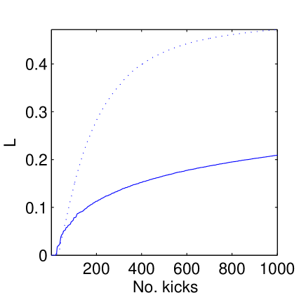
Figure 16: (Color online) Total quantum (solid blue line) and classical (blue dots) probabilities for scattering to the left of the island $\left(x<-x_{b}\right)$ as a function of the number of kicks. $K=1$, $\tau=0.01$, $x_{0}=-2$, $p_{0}=0$.

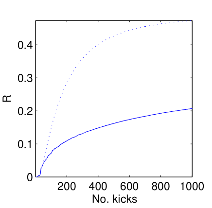
Figure 17: (Color online) Total quantum (solid blue line) and classical (blue dots) probabilities for scattering to the right of the island $\left(x>x_{b}\right)$ as a function of the number of kicks. $K=1$, $\tau=0.01$, $x_{0}=-2$, $p_{0}=0$.

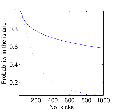
Figure 18: Total quantum (solid blue line) and classical (blue dots) probabilities to stay in the island $\left(\left|x\right|\leq x_{b}\right)$ as a function of the number of kicks. $K=1$, $\tau=0.01$, $x_{0}=-2$, $p_{0}=0$.

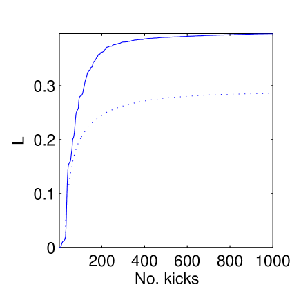
Figure 19: Total quantum (solid blue line) and classical (blue dots) probabilities for scattering to the left of the island $\left(x<-x_{b}\right)$ as a function of the number of kicks. $K=1$, $\tau=0.01$, $x_{0}=-3$, $p_{0}=0$.

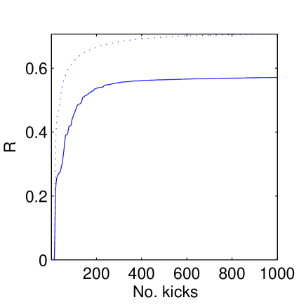
Figure 20: Total quantum (solid blue line) and classical (blue dots) probabilities for scattering to the right of the island $\left(x>x_{b}\right)$ as a function of the number of kicks. $K=1$, $\tau=0.01$, $x_{0}=-3$, $p_{0}=0$.

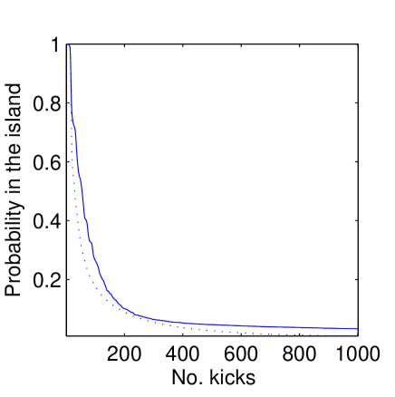
Figure 21: Total quantum (solid blue line) and classical (blue dots) probabilities to stay in the island $\left(\left|x\right|\leq x_{b}\right)$ as a function of the number of kicks. $K=1$, $\tau=0.01$, $x_{0}=-3$, $p_{0}=0$.

we compare the quantum and classical scattering of a wavepacket launched from the left of the main island. We notice that there is a substantial difference, which decreases when we decrease the effective Planck’s constant, $\tau$. Figures 16-18 and Figs. 19-21 differ in the initial launching position of the wavepacket ($x_{0}=-2$, for Figs. 16-18 and $x_{0}=-3$ for Figs. 19-21). We notice that the scattering is sensitive to $x_{0}$. Different aspects of chaotic scattering for this problem were explored in Jensen1992 , and in particular, the effect of small $\hbar$ on washing out rainbow singularities of the classical scattering function.

VII Discussion and Conclusions

VII.1 Discussion of experimental realizability

In the present work the classical and quantum dynamics of a system with a mixed phase space were studied. It is proposed to realize this system by injecting cold atoms into a coherent, pulsed, gaussian light beam. The phase space structures, which can be seen on Figs. 1,2 and 7 are controlled by the parameters of the beam via the parameter $K$. Since it is relatively straightforward to control the parameters of gaussian beams, the proposed system is ideal for the exploration of dynamics of mixed systems. In what follows limitations on experimental realizations are discussed. First we consider the realizability of an approximately one dimensional situation necessary for the validity of our theoretical results. Let us assume that the gaussian beam propagates in the $z$ direction. Its profile in the $xy$ plane is

$$e^{-\frac{x^{2}}{2\Delta^{2}}-\frac{y^{2}}{2\Delta_{y}^{2}}}.$$ (34)

Assuming that the extent of the light beam is much smaller than the Rayleigh length, $z_{R}=\pi\Delta^{2}/\lambda$ where $\lambda$ is the wavelength, and the $z$ dependence of the potential can be ignored. The potential of Eq. (34) can be well approximated by $\exp\left(-x^{2}/\left(2\Delta^{2}\right)\right)$ in (1), for sufficiently small values of $y^{2}/\Delta_{y}^{2}$, and, to facilitate this, it is appropriate to consider $\Delta_{y}\gg\Delta$, i.e., a quasi-sheet-like beam. Such beams are experimentally realizable via routine methods. To analyze this situation, the normalized map $M$ of (5) should be replaced by one with $\exp\left(-x^{2}/2\right)$ replaced by $\exp\left(-\left[x^{2}/2+y^{2}\left(\Delta/\Delta_{y}\right)^{2}\right]\right)$. In addition, there are equations for $y_{n}$ and its conjugate momentum $p_{y,n}$, which in dimensionless units with $y$ and $p_{y,n}$ rescaled by $\Delta$ and $T/\left(m\Delta\right)$, respectively, take the form,

$$p_{y,n+1} = p_{y,n}-K_{y}y_{n}e^{-\frac{x_{n}^{2}}{2}-\frac{1}{2}\left(\frac{\Delta}{\Delta_{y}}\right)^{2}y_{n}^{2}},$$

$$y_{n+1} = y_{n}+p_{y,n+1},$$ (35)

where

$$K_{y}=K\left(\frac{\Delta}{\Delta_{y}}\right)^{2}.$$ (36)

Since $K\approx 1$ and $\Delta/\Delta_{y}\ll 1$, it can be assumed that $K_{y}\ll 1$. Therefore, the motion in the $y$ direction is slow relative to the motion in the $x$ direction. Thus $\exp\left(-x_{n}^{2}/2\right)$ can be approximated by its time average $\left\langle\exp\left(-x^{2}/\left(2\Delta^{2}\right)\right)\right\rangle\equiv\rho$ (which is of order unity), and, for sufficiently small $y$ the $y-$motion (35) can be described by a Harmonic oscillator with a force constant $2K_{y}\rho\ll 1$. Conservation of energy $E_{y}$ implies that the maximal value of $y$ satisfies

$$E_{y}=2K_{y}\rho y_{\mathrm{max}}^{2}.$$ (37)

The energy $E_{y}$ is determined by the initial preparation. Let us assume that initially the atoms form a Bose-Einstein Condensate (BEC) and are in a harmonic trap that is anisotropic where the frequency in the $y$ direction is $\nu_{y}^{\prime}$ in experimental units, and $\nu_{y}=T\nu_{y}^{\prime}$ in our rescaled units. We assume that the center of this trap $y_{0}$ satisfies $y_{0}\ll y_{max}$. The experiment starts when the trap is turned off. Assuming the atoms are in the ground state, their energy in our rescales units is

$$\frac{1}{2}\hbar\nu_{y}^{\prime}\left(\frac{T^{2}}{m\Delta^{2}}\right)=\frac{1}{2}\nu_{y}\tau\leq E_{y}.$$ (38)

We desire the effect of the motion in the $y$ direction on the motion in the $x$ direction (Eq.(1) with $\exp\left(-x^{2}/\left(2\Delta^{2}\right)\right)$ replaced by $V$ of (34)) to be negligible. Thus it is required that

$$\eta\equiv y_{\mathrm{max}}^{2}\left(\frac{\Delta}{\Delta_{y}}\right)^{2}\ll 1.$$ (39)

In this case the $y$ motion corresponds to a variation in $K$ of the order $\Delta K\sim K\eta$. Using (37) and (38), condition (39) reduces to

$$\frac{1}{4}\frac{\nu_{y}\tau}{K}\leq\frac{E_{y}}{2K}=\eta\ll 1,$$ (40)

where, since we are interested only in crude estimates, we have replaced $\rho$ by one. The initial spread in $y$ is given by the ground state of the harmonic oscillator, where $\left\langle y^{2}\right\rangle=\tau/\left(2\nu_{y}\right)$, and we require that the expectation value of $y^{2}$ satisfies $\left\langle y^{2}\right\rangle\ll y_{\mathrm{max}}^{2}$, resulting in

$$\left(\frac{\Delta}{\Delta_{y}}\right)^{2}\frac{\tau}{2\nu_{y}}\ll\eta.$$ (41)

For both inequalities (40) and (41) to be satisfied it is required that

$$\left(\frac{\Delta}{\Delta_{y}}\right)^{2}\frac{\tau}{2\eta}\ll\nu_{y}\leq\frac{4K}{\tau}\eta.$$ (42)

The resulting fundamental lower bound on $\eta$ is

$$\left(\frac{\Delta}{\Delta_{y}}\right)^{2}\frac{\tau^{2}}{8K}\ll\eta.$$ (43)

Reasonable experimental values are $\Delta/\Delta_{y}\approx 10^{-2}$ and $\nu_{y}\approx 0.1$. For $\tau=10^{-2}$ and $K\approx 1$ the lower bound on $\eta$ is $10^{-5}$ leaving a wide range for ‘engineering’ of BEC traps so that the $\nu_{y}$ is in the range (42). For $\nu_{y}\approx 0.1$ and $\tau=10^{-2}$ and $K\approx 1$ we can make $\eta\lesssim 10^{-3}$. Since this value of $\eta$ is small compared to the value of $\Delta K=K_{2}-K_{1}$, used in our fidelity calculations (Figs 3, 5, 11, 12), those calculations are expected to be uneffected by $y$ motion for our assumed parameters. It is also encouraging to see that noise of a higher level does not destroy fidelity oscillations (see Fig. 12). One should note, however, that the variation of the effective $K$ of the motion in the $x$ direction is slow, with effective frequency $\Delta/\Delta_{y}$ that for $\Delta/\Delta_{y}\approx 10^{-2}$ is of order $10^{-2}$. For these reasons, we expect that, the model that we have explored theoretically in the present work should be realizable for a wide range of experimental parameters.

VII.2 Conclusions

The main result of this paper is that the quantum fidelity is sensitive to the phase space details that are finer than Planck’s constant, contrary to expectations of Refs. Berry1972 ; Berry1977c . In particular, the fidelity was studied and predicted to oscillate with frequencies that can be predicted from classical considerations. This behavior is characteristic of regular regions. Fidelity exhibits a periodic sequence of peaks. For wavepackets in the main island, it was checked that the peak structure is stable in the presence of external noise but the amplitude decays with time. For wavepackets initialized in a chain of regular islands, it was found that the fidelity exhibits several time scales that can be predicted from classical considerations. For wavepackets initialized in the chaotic region, the fidelity is found to decay exponentially as expected. It was shown how quasi-energies are related to classical structures in phase space. Substantial deviation between quantum and classical scattering was found. These quantum mechanical effects can be measured with kicked gaussian beams as demonstrated in the present work.

- (1) M. Tabor. Chaos and integrability in nonlinear dynamics : an introduction. Wiley-Interscience, New York, 1989.
- (2) A. M. Ozorio de Almeida. Hamiltonian systems : chaos and quantization. Cambridge University Press, Cambridge, 1988.
- (3) G. Casati, I. Guarneri, and U . Smilansky, editors. Proc. Internat. School Phys. Enrico Fermi, volume CXIX, Varenna, July 1991. North-Holland.
- (4) M. C. Gutzwiller. Chaos in Classical and Quantum Mechanics. Springer, New York, 1990.
- (5) G.L Oppo, S.M. Barnett, E. Riis, and M. Wilkinson, editors. Proc. of the 44-th Scottish Universities Summer School in Physics. Springer, August 1994.
- (6) F. Haake. Quantum Signatures of Chaos. Springer, Berlin, 2001.
- (7) E. Ott. Chaos in Dynamical Systems. Cambridge University Press, Cambridge, 2002.
- (8) M.V. Berry and M. Tabor. Closed orbits and regular bound spectrum. Proc. Roy. Soc. London Ser. A, 349(1656):101–123, 1976.
- (9) M.V. Berry and M. Tabor. Calculating bound spectrum by path summation in action-angle variables. J. Phys. A, 10(3):371–379, 1977.
- (10) M.V. Berry and M. Tabor. Level clustering in regular spectrum. Proc. Roy. Soc. London Ser. A, 356(1686):375–394, 1977.
- (11) O. Bohigas, M. J. Giannoni, and C. Schmit. Characterization of chaotic quantum spectra and universality of level fluctuation laws. Phys. Rev. Lett., 52(1):1–4, Jan 1984.
- (12) M. Sieber and K. Richter. Correlations between periodic orbits and their role in spectral statistics. Phys. Scripta, 2001(T90):128, 2001.
- (13) S. Müller, S. Heusler, P. Braun, F. Haake, and A. Altland. Semiclassical foundation of universality in quantum chaos. Phys. Rev. Lett., 93(1):014103, Jul 2004.
- (14) M.V. Berry and M. Robnik. Semiclassical level spacings when regular and chaotic orbits coexist. J. Phys. A, 17(12):2413–2421, 1984.
- (15) J. H. Jensen. Convergence of the semiclassical approximation for chaotic scattering. Phys. Rev. Lett., 73(2):244–247, Jul 1994.
- (16) J. H. Jensen. Quantum corrections for chaotic scattering. Phys. Rev. A, 45(12):8530–8535, Jun 1992.
- (17) F.L. Moore, J.C. Robinson, C.F. Bharucha, B. Sundaram, and M.G. Raizen. Atom optics realization of the quantum delta-kicked rotor. Phys. Rev. Lett., 75(25):4598–4601, Dec 1995.
- (18) A. Peres. Stability of quantum motion in chaotic and regular systems. Phys. Rev. A, 30(4):1610–1615, Oct 1984.
- (19) R. A. Jalabert and H. M. Pastawski. Environment-independent decoherence rate in classically chaotic systems. Phys. Rev. Lett., 86(12):2490–2493, Mar 2001.
- (20) Ph. Jacquod, I. Adagideli, and C. W. J. Beenakker. Decay of the Loschmidt echo for quantum states with sub-Planck-scale structures. Phys. Rev. Lett., 89(15):154103, Sep 2002.
- (21) T. Gorin, T. Prosen, T. H. Seligman, and M. Znidaric. Dynamics of Loschmidt echoes and fidelity decay. Phys. Rep., 435(2-5):33–156, 2006.
- (22) E. Ott, T. M. Antonsen, and J. D. Hanson. Effect of noise on time-dependent quantum chaos. Phys. Rev. Lett., 53(23):2187–2190, 1984.
- (23) D. Cohen. Quantum chaos, dynamical correlations, and the effect of noise on localization. Phys. Rev. A, 44(4):2292–2313, Aug 1991.
- (24) R. Blumel and U. Smilansky. Classical irregular scattering and its quantum-mechanical implications. Phys. Rev. Lett., 60(6):477–480, FEB 8 1988.
- (25) R. A. Jalabert, H. U. Baranger, and A. D. Stone. Conductance fluctuations in the ballistic regime - a probe of quantum chaos. Phys. Rev. Lett., 65(19):2442–2445, NOV 5 1990.
- (26) E. Doron, U. Smilansky, and A. Frenkel. Chaotic scattering and transmission fluctuations. Phys. D, 50(3):367–390, JUL 1991.
- (27) Y. C. Lai, R. Blumel, E. Ott, and C. Grebogi. Quantum manifestations of chaotic scattering. Phys. Rev. Lett., 68(24):3491–3494, JUN 15 1992.
- (28) M.V. Berry and K.E. Mount. Semiclassical approximations in wave mechanics. Rep. Progr. Phys., 35(4):315, 1972.
- (29) M.V. Berry. Semiclassical mechanics in phase space - study of wigners function. Philos. Trans. Roy. Soc. London Ser. A, 287(1343):237–271, 1977.
- (30) J.D. Hanson, E. Ott, and T.M. Antonsen. Influence of finite wavelength on the quantum kicked rotator in the semiclassical regime. Phys. Rev. A, 29(2):819–825, 1984.
- (31) S. Tomsovic and D. Ullmo. Chaos-assisted tunneling. Phys. Rev. E, 50(1):145–162, Jul 1994.
- (32) M. Sheinman, S. Fishman, I. Guarneri, and L. Rebuzzini. Decay of quantum accelerator modes. Phys. Rev. A, 73(5):052110, May 2006.
- (33) S. Löck, A. Bäcker, R. Ketzmerick, and P. Schlagheck. Regular-to-chaotic tunneling rates: From the quantum to the semiclassical regime. Phys. Rev. Lett., 104(11):114101, Mar 2010.
- (34) N. R. Cerruti and S. Tomsovic. Sensitivity of wave field evolution and manifold stability in chaotic systems. Phys. Rev. Lett., 88(5):054103, Jan 2002.
- (35) S. Wimberger and A. Buchleitner. Saturation of fidelity in the atom-optics kicked rotor. J. Phys. B, 39(7):L145, 2006.
- (36) M. F. Andersen, T. Grünzweig, A. Kaplan, and N. Davidson. Revivals of coherence in chaotic atom-optics billiards. Phys. Rev. A, 69(6):063413, Jun 2004.
- (37) A. Kaplan, M.F. Andersen, T. Grünzweig, and N. Davidson. Hyperfine spectroscopy of optically trapped atoms. J. Opt. B, 7(8):R103, 2005.
- (38) M. F. Andersen, A. Kaplan, T. Grünzweig, and N. Davidson. Decay of quantum correlations in atom optics billiards with chaotic and mixed dynamics. Phys. Rev. Lett., 97(10):104102, Sep 2006.
- (39) M. A. Nielsen and I. L. Chuang. Quantum computation and quantum information. Cambridge University Press, Cambridge, 2000.
- (40) M. V. Berry, N. L. Balazs, M. Tabor, and A. Voros. Quantum maps. Ann. Physics, 122(1):26 – 63, 1979.
- (41) W.K. Hensinger, H. Haffer, A. Browaeys, N.R. Heckenberg, K. Helmerson, C. McKenzie, G.J. Milburn, W.D. Phillips, S.L. Rolston, H. Rubinsztein-Dunlop, and B. Upcroft. Dynamical tunnelling of ultracold atoms. Nature, 412(6842):52–55, Jul 2001.
- (42) D.A. Steck, W.H. Oskay, and M.G. Raizen. Observation of chaos-assisted tunneling between islands of stability. Science, 293(5528):274–278, Jul 2001.
- (43) D.A. Steck, W.H. Oskay, and M.G. Raizen. Fluctuations and decoherence in chaos-assisted tunneling. Phys. Rev. Lett., 88(12), Mar 2002.
- (44) V. Averbukh, N. Moiseyev, B. Mirbach, and H. J. Korsch. Dynamical tunneling through a chaotic region. Z. Phys. D, 35:247–256, 1995. 10.1007/BF01745527.
- (45) V. Averbukh, S. Osovski, and N. Moiseyev. Controlled tunneling of cold atoms: From full suppression to strong enhancement. Phys. Rev. Lett., 89(25):253201, Nov 2002.
- (46) S. Osovski and N. Moiseyev. Fingerprints of classical chaos in manipulation of cold atoms in the dynamical tunneling experiments. Phys. Rev. A, 72(3), Sep 2005.
- (47) J. M. Greene. A method for determining a stochastic transition. J. Math. Phys., 20:1183, 1979.
- (48) H. Rebecca, O. Tali, Y. S. Avizrats, A. Iomin, S. Fishman, and I. Guarneri. Regimes of stability of accelerator modes. Phys. D, 226(1):1 – 10, 2007.