Nonlinear Waves in Lattices: Past, Present, Future

Abstract

In the present work, we attempt a brief summary of various areas where nonlinear waves have been emerging in the phenomenology of lattice dynamical systems. These areas include nonlinear optics, atomic physics, mechanical systems, electrical lattices, nonlinear metamaterials, plasma dynamics and granular crystals. We give some of the recent developments in each one of these areas and speculate on some of the potentially interesting directions for future study.

1 Introduction

Over the last two decades, there has been an explosion of interest on the dynamics of nonlinear waves in lattices. It can be argued that this field was actually initiated by the seminal investigation of Fermi, Pasta and Ulam (FPU) presented in ?, who posed the following question: How long does it take for long-wavelength oscillations to transfer their energy into an equilibrium distribution in a one-dimensional string of nonlinearly interacting particles? This question spurred the activity of a wide array of fields including soliton theory, discrete lattice dynamics and KAM theory, all of which remain active research fields today.

The development of soliton theory, while focusing at the continuum level at first through the investigations of ? and the concomitant developments of the theory of integrability for the Korteweg-de Vries equation, also offered some of the first particularly interesting examples of lattice nonlinear dynamical systems. Among the prime examples thereof, one can classify the Toda lattice of ?, the Ablowitz-Ladik equation of ? and the Calogero-Moser $N$-body problem, see e.g. the works of ? and ?.

It was at around the same time that some of the early fundamental suggestions of the role of discrete solitons in physical systems were made in the 1970s. Some of the pioneers of these contributions were Davydov, see e.g. ? and Heeger and collaborators, see e.g. ? and ?. Davydov proposed the discrete soliton as a tool for understanding energy transfer in proteins and their $\alpha$-helices, while Heeger and collaborators put forth solitonic models for understanding neutral and charge transport in conducting polymer chains such as polyacetylene and polythiophene.

However, a true explosion of the field came about in the late 1980s when not only major developments arose in the context of the so-called discrete self-trapping equation of ?, but also the work of ? and ? brought forth the theme of intrinsic localized modes (or discrete breathers) in anharmonic lattices. Although this theme had been explored earlier e.g., by ?, ? and ?, it was ? and ? that motivated a number of other researchers to explore the existence and stability of such modes more thoroughly and to start obtaining fundamental results about their properties, as well as to devise special limits (such as the anti-continuum (AC) limit of lattices with uncoupled sites) which could be used to showcase the generic nature of these modes. A landmark in connection to these efforts was the work of ? which established rigorously the existence/robustness of such localized modes starting from the AC limit, under minimal appropriate (non-resonance) assumptions for chains of nonlinear oscillators.

Since these early steps, there has been a tremendous amount of developments in the area of nonlinear waves in dynamical lattices. This activity has chiefly been fueled by the experimental observation of these modes in a wide range of physical systems in biophysics, solid state physics, nonlinear optics, atomic physics, granular crystals, and plasma physics, in addition to numerous developments in the more classical fields of mechanical and electrical lattices [and even the latter have seen interesting recent developments e.g. with the emergence of the field of nonlinear metamaterials, among others, as discussed in section LABEL:future1 below]. A (partial) list of key physical systems where explanations in terms of nonlinear waves in lattices have had an impact includes:

• The observation of discrete breathers in complex electronic materials such as halide-bridged transition metal complexes as e.g. in ?.

• The formation of denaturation bubbles in the DNA double strand dynamics summarized e.g. in ?.

• The emergence of dynamical instabilities, discrete quantum self-trapping and localized modes in ultracold Bose-Einstein condensates in the presence of deep optical lattices, see e.g. the reviews of ? and ?.

• The illustration of localized modes of solitonic, vortex, ring, multipole, surface, gap, necklace and numerous other types in the nonlinear optics of evanescently coupled waveguide arrays, as well as in that of biased photorefractive crystals; a relevant recent review can be found in ?.

• The prototypical mechanical realization of solitary waves and localized modes in driven micromechanical cantilever arrays as shown in ?, as well as in coupled torsion pendula where a recent example is given by ?.

• The examination of interesting properties and mobility of localized modes in nonlinear electrical lattices and transmission lines; see e.g. ? and ?.

• The presence of nearly compact solitary waves in granular crystals consisting of beads with Hertzian elastic interactions reviewed in ? and ?.

• The creation of discrete breather type structures in layered antiferromagnetic samples such as those of a (C${}_{2}$H${}_{5}$NH${}_{3}$)${}_{2}$CuCl${}_{4}$ crystal, upon imposition of a dynamically unstable continuous wave (which falls into modulational instability and results in the localized waveforms); see the relevant works of ? and ?.

These experimental developments have, in turn, motivated a huge range of theoretical advances in connection to the properties and interactions of these lattice nonlinear waves and on how these are modified in comparison to their continuum siblings. In particular, some of the areas that have seen intense theoretical activity concern:

• The existence and stability of the localized modes.

• The dynamics and interactions of multiple such states in nonlinear lattices.

• The effect of external potentials (either local “impurity-like” potentials, or more broad externally imposed, field potentials)

• The effect of short-range (local) versus long-range (nonlocal) interactions.

• The presence of excitation thresholds for such nonlinear states (especially in higher dimensional settings).

• The statistical mechanics and long-time asymptotics of these lattice systems and the role of the localized modes in them.

• The effects of disorder and the role of the interplay between the linear phenomenon of Anderson localization and of the nonlinearity-induced type of localization.

• The interaction with and scattering of phonon-like modes from discrete solitary waves.

• The modifications imparted on the waveforms of such localized states and the new possibilities for ones such (e.g. with embedded vorticity) afforded by higher dimensional settings.

Many of these topics have been summarized in a number of reviews by ?, ?, ?, ?, ?, ?, ? and more recently in a number of books e.g. about Klein-Gordon nonlinear lattices by ?, as well as about nonlinear Schrödinger ones by ?.

As it can be inferred from the shear volume of review articles on the topic (as well as that of full-blown books), it is impossible to give an exhaustive description of any particular aspect or application of the subject in anything less than a lengthy review or a book. Our aim herein will thus, by necessity, be more modest, but in some sense, also more “forward looking”. We aim to give a selective presentation of some of recent developments of a few among these areas, which in the present author’s evaluation hold significant potential for future developments in the field of localized modes, nonlinear waves and discrete breathers. Obviously, this bears a significant weight of subjective perception and a personalized viewpoint about which we caution the reader in advance. On the other hand, our hope is to offer a number of interesting directions for future study in these areas which could significantly enhance our understanding of nonlinear waves in these settings, promoting their state-of-the-art and offering significant connections with present or near-future experimental settings and potentially also with applications.

We will categorize our presentation based on the different models and the corresponding areas of interest. Hence, upon introducing our basic notation, the third section will concern itself with localized modes in models of the discrete nonlinear Schrödinger type and their applications in nonlinear optics and atomic physics. The fourth section will consider models of the Klein-Gordon type, as well as their mechanical and electrical (as well as nonlinear metamaterial) applications. The fifth section will focus on models of the FPU type arising in the examination of granular crystals with Hertzian (or modified Hertzian) interactions, as well as in the case of study of dusty plasmas. Lastly, in section six, we will summarize some of our discussion and offer some concluding thoughts.

2 Notation

The prototypical dynamical lattices that will be considered in this review will be the discrete nonlinear Schrödinger equation (DNLS) in the form:

$$i\dot{u}_{n}=-\epsilon(u_{n+1}+u_{n-1})-|u_{n}|^{2}u_{n},$$ (2.1)

the nonlinear Klein-Gordon (KG) lattice of the form:

$$\ddot{u}_{n}=\epsilon(u_{n+1}+u_{n-1}-2u_{n})-V^{\prime}(u_{n}),$$ (2.2)

and the FPU-type dynamical lattice of the form

$$\ddot{u}_{n}=V^{\prime}(u_{n+1}-u_{n})-V^{\prime}(u_{n}-u_{n-1}),$$ (2.3)

where $u_{n}$ is the dynamical variable of interest measured at site $n$, $\epsilon$ is the coupling parameter and $V$ a potential (that could be onsite for KG lattices or inter-site for FPU ones).

It should be noted that in what follows, we will not restrict ourselves to the one-dimensional framework of Eqs. (2.1)-(2.3), but motivated by physical applications, we will often consider higher dimensional variants of the models. In their prototypical form, two-dimensional generalizations of Eqs. (2.1)-(2.3) read

$$i\dot{u}_{n,m}=-\epsilon(u_{n+1,m}+u_{n-1,m}+u_{n,m+1}+u_{n,m-1})-|u_{n,m}|^{2}u_{n,m},$$ (2.4)

for the DNLS lattice,

$$\ddot{u}_{n,m}=\epsilon(u_{n+1,m}+u_{n-1,m}+u_{n,m+1}+u_{n,m-1}-4u_{n,m})-V^{\prime}(u_{n,m}),$$ (2.5)

for the KG case, while for the FPU-type lattices we have

$$\ddot{u}_{n,m}=V^{\prime}(u_{n+1,m}-u_{n,m})-V^{\prime}(u_{n,m}-u_{n-1,m})+V^{\prime}(u_{n,m+1}-u_{n,m})-V^{\prime}(u_{n,m}-u_{n,m-1}).$$ (2.6)

This, in turn, clearly suggests how to expand the model beyond two dimensions and into the three- or arbitrary-dimensional-case, by sequentially adding more lattice directions and linear (in cases such as (2.4)-(2.5)) or nonlinear (as in case (2.6)) interactions along them.

In the first one of these, the field will be complex and we will most often seek stationary (standing wave) type solutions of the form $u_{n}=\exp(i\mu t)v_{n}$; $\mu$ is often referred to as the propagation constant in nonlinear optics, or the chemical potential in Bose-Einstein condensates and characterizes the frequency of such standing wave solutions. These will satisfy the steady state equation:

$$(\mu-|v_{n}|^{2})v_{n}=\epsilon(v_{n+1}+v_{n-1}).$$ (2.7)

Additionally, one of the fundamental ideas that we will use in exploring this class of systems will be that of the anti-continuum limit of ?. This is the limit where the sites are uncoupled with $\epsilon=0$. In this case, Eq. (2.7) is completely solvable $v_{n}=0,\pm\sqrt{\mu}\exp(i\theta_{n})$, where $\theta_{n}$ is a free phase parameter for each site. The fundamental question of interest will involve the persistence of these solutions for $\epsilon\neq 0$, as well as their stability. The latter will be often explored by means of linear stability analysis, upon imposition of a perturbation of the form:

$$u_{n}(t)=\exp(i\mu t)\left[v_{n}+\delta\left(p_{n}\exp(\lambda t)+q_{n}^{\star}\exp(\lambda^{\star}t)\right)\right].$$ (2.8)

[Notice that the ${}^{\star}$ will be generally used in what follows to denote complex conjugation.] Consideration of the resulting equation upon substitution of (2.8) to (2.1), at ${\cal O}(\delta)$ yields the linearization (infinite-dimensional matrix) eigenvalue problem for the eigenvalues $\lambda$ and eigenvectors $(p_{n},q_{n})$.

In the case of the Klein-Gordon models, we will focus on discrete breather time-periodic solutions for different potentials which are either polynomials in the form $V(u_{n})=\sum_{n=2}^{N}a_{j}u_{n}^{j}$ or other functions such as $V(u_{n})=1-\cos(u_{n})$ (in the sine-Gordon case). Notice also that we will often use the operator notation $\Delta_{2}u_{n}=u_{n+1}+u_{n-1}-2u_{n}$ for the discrete Laplacian. For the FPU lattices, we will primarily concern ourselves with power law potentials and particularly the Hertzian elastic case of $V(r_{n})\sim r_{n}^{5/2}$, but we will also briefly refer to other potentials such as the Yukawa one $V(r_{n})\sim\exp(-\alpha r_{n})/r_{n}$ (for $r_{n}>0$) in the context of dusty plasmas. Notice that in the FPU-type chains, we will also refer to the so-called strain formulation which introduces the modified field variable $r_{n}=u_{n-1}-u_{n}$ and leads to the dynamical equation

$$\ddot{r}_{n}=V^{\prime}(r_{n+1})+V^{\prime}(r_{n-1})-2V^{\prime}(r_{n}).$$ (2.9)

3 DNLS Models in Nonlinear Optics and Atomic Physics

3.1 Recent Developments

Many of the investigations in these fields stemmed from the relevance of the DNLS model and its variants in the nonlinear optics of fabricated AlGaAs waveguide arrays as in ?, as well as in that of Bose-Einstein condensates in sufficiently deep optical lattices analyzed in ?, ?, and ?.

In the former area, a multiplicity of phenomena such as discrete diffraction, Peierls barriers (the energetic barrier that a wave needs to overcome to move from one lattice site to the next), diffraction management (the periodic alternation of the diffraction coefficient) in ? and gap solitons (structures localized due to nonlinearity in the gap of the underlying linear spectrum) in ? among others [see also ?] were experimentally observed. More recently, fundamental investigations also on the modulational instability arising in such settings for simple plane wave solutions in ?, and on the role of multiple components and possible four-wave-mixing effects arising from their coupling in ? have been explored, as well as that of interactions of solitary waves with surfaces in ?.

A related area where lattice dynamical models, although not directly relevant as the most appropriate description (since the setting is, in principle continuum with a periodic potential), still yield accurate predictions regarding the existence and the stability of nonlinear localized modes is that of optically induced lattices in photorefractive media such as Strontium Barium Niobate (SBN). Since the theoretical suggestion of such lattices in ?, and their experimental realization in ?, ? and ?, there has been a tremendous growth in the area of nonlinear waves and solitons in such periodic, predominantly two-dimensional, lattices. The continuously growing array of structures that have been predicted and experimentally obtained in such lattices includes (but is not limited to) various discrete multi-pulse patterns, such as the discrete dipole solitons in ?, quadrupole solitons in ?, necklace solitons in ?, soliton stripes in ?, discrete vortices in ?, and ?, rotary solitons in ?, surface solitons in ?, and so on. Such structures have a definite potential to be used as carriers and conduits for data transmission and processing, in the setting of all-optical communication schemes; see a detailed recent review in ?.

Lastly, a completely independent and entirely different field where relevant considerations and structures, as well as models of the DNLS type arise is that of ultracold atomic gases in the form of Bose-Einstein condensates (BECs) under the confinement imposed by so-called optical lattice potentials. These are periodic traps produced by counter-propagating laser beams in one, two or even all three directions, see e.g. ?. This field has also experienced a tremendous amount of development in the past few years with some of its landmarks being the prediction [in ?] and manifestation [in ?] of modulational instabilities, the observation of gap solitons in ?, of Landau-Zener tunneling (tunneling between different bands of the periodic potential) in ? and Bloch oscillations (for matter waves subject to combined periodic and linear potentials) in ? among many other salient features.

All of the above settings are described at some level of approximation by a continuum nonlinear Schrödinger (NLS) equation with a periodic potential. However, when the periodic potential is sufficiently deep, it was realized that an equivalent description of the system can be given by a nonlinear dynamical lattice as discussed e.g. in ?, and ?. This was further elaborated for BEC settings in ? [see also ? for a related discussion in connection to nonlinear optics], whose presentation we briefly follow here.

The localized wavefunctions at the wells of the periodic potential can be approximated by Wannier functions, i.e., the Fourier transform of Bloch functions. Given the completeness of the Wannier basis, any solution of the NLS equation with a periodic potential can be expressed as $u(x,t)=\sum_{n,\alpha}c_{n,\alpha}(t)w_{n,\alpha}(z)$, where $n$ and $\alpha$ label wells and bands of the periodic potential, respectively.

Substituting the above expression into the dynamical equation, and using the orthonormality of the Wannier basis as indicated in ?, we obtain a set of differential equations for the coefficients. Upon suitable decay of the Fourier coefficients and the Wannier functions’ prefactors (which can be systematically checked for given potential parameters), the model can be reduced to

$$i{\frac{dc_{n,\alpha}}{dt}}=\hat{\omega}_{0,\alpha}c_{n,\alpha}+\hat{\omega}_{1,\alpha}\left(c_{n-1,\alpha}+c_{n+1,\alpha}\right)+\sum_{\alpha_{1},\alpha_{2},\alpha_{3}}W^{nnnn}_{\alpha\alpha_{1}\alpha_{2}\alpha_{3}}c_{n,\alpha_{1}}^{\ast}c_{n,\alpha_{2}}c_{n,\alpha_{3}},$$ (3.1)

where $W^{nn_{1}n_{2}n_{3}}_{\alpha\alpha_{1}\alpha_{2}\alpha_{3}}=\int_{-\infty}^{\infty}w_{n,\alpha}w_{n_{1},\alpha_{1}}w_{n_{2},\alpha_{2}}w_{n_{3},\alpha_{3}}dx$ is the Wannier function overlap integral and

$$\hat{\omega}_{n,\alpha}=\frac{L}{2\pi}\int_{-\pi/L}^{\pi/L}E_{\alpha}(k)e^{-iknL}dk\,,$$ (3.2)

is the Fourier transform of the energy $E_{\alpha}(k)$ of the Bloch mode corresponding to wavenumber $k$ for a potential of spatial period $L$. This degenerates into the so-called tight-binding model

$$\hskip-28.45274pti\frac{dc_{n,\alpha}}{dt}=\hat{\omega}_{0,\alpha}c_{n,\alpha}+\hat{\omega}_{1,\alpha}\left(c_{n-1,\alpha}+c_{n+1,\alpha}\right)+W^{nnnn}_{1111}|c_{n,\alpha}|^{2}c_{n,\alpha},$$ (3.3)

i.e., the DNLS equation, when restricting consideration to the first band. Higher-dimensional versions of the latter are of course physically relevant models and have, therefore, been used in various studies concerning quasi-2D and 3D BECs confined in strong optical lattices as illustrated in ? and similarly in 2D waveguide arrays as summarized in ?.

The relevance of the DNLS model in this wide array of application areas prompted an intense activity in investigating the fundamental solitary wave solutions of the model. We now focus on analyzing these prototypical solutions and their stability in the context of Eq. (2.1). In particular, for stationary solutions, upon multiplying Eq. (2.7) by $v_{n}^{\ast}$ and subtracting the complex conjugate of the resulting equation leads to:

$$v_{n}^{\ast}v_{n+1}-v_{n}v_{n+1}^{\ast}={\rm const.}~{}~{}\Rightarrow~{}~{}2{\rm arg}(v_{n+1})=2{\rm arg}(v_{n}),$$ (3.4)

for localized solutions (i.e., vanishing as $n\rightarrow\pm\infty$). Using the scaling freedom of the equation to set $\mu=1$ allows us to infer that the only states that will persist for finite $\epsilon$ will be the ones containing sequences with combinations of $v_{n}=\pm 1$ and $v_{n}=0$. The work of ? provided a systematic numerical classification of the most fundamental of the resulting sequences and their bifurcations. Some of the prototypical examples of sequences involving one, two and three sites are illustrated in Fig. 1. While in our discussion below, we restrict our consideration to the case of focusing nonlinearity, our results can be extended to the defocusing case [with the opposite sign of the nonlinearity in Eq. (2.1)] via the so-called staggering transformation $w_{n}=(-1)^{n}u_{n}$. This converts the defocusing nonlinearity into a focusing one, with an appropriate frequency rescaling which can be trivially absorbed in a phase or gauge transformation.

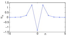
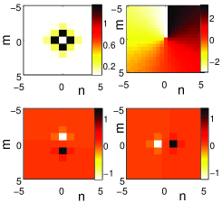
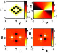
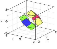
Figure 1: (Color online) A sampler of solutions of the discrete nonlinear Schrödinger equation in 1-, 2- and 3-spatial lattice dimensions. The top left shows the always stable fundamental single soliton. The top middle and right show the out-of-phase two- and three-site excitations (which can be stable near the anti-continuum limit). The bottom left (4-panel set including the amplitude, phase, real and imaginary part contour plots of the solution) shows the prototypical vortex of topological charge $S=1$ (which is also stable near the AC limit). The bottom middle panel contains a rhombic $S=2$ generalization thereof with $8$ sites (which may also be stable), while the bottom right contains the also stable near the AC limit 6-site diamond three-dimensional configuration.

We now turn to the examination of stability. Using the linearization ansatz of Eq. (2.8) and a simple eigenvector rotation leads to the equivalent symplectic formalism of the linear stability problem $J{\cal L}w=\lambda w$, where ${\cal L}$ is a diagonal, self-adjoint matrix with the operators ${\cal L}_{+}$ and ${\cal L}_{-}$ given below in its diagonal entries and $J$ is the symplectic matrix. ${\cal L}_{+}$ and ${\cal L}_{-}$ are defined by:

$$(1-3v_{n}^{2})a_{n}-\epsilon(a_{n+1}+a_{n-1}) = {\cal L}_{+}a_{n}=-\lambda b_{n}$$ (3.5)

$$(1-v_{n}^{2})b_{n}-\epsilon(b_{n+1}+b_{n-1}) = {\cal L}_{-}b_{n}=\lambda a_{n}.$$ (3.6)

Using once again the AC limit, we assume a $v_{n}$ with $N$ “excited” (i.e., $\neq 0$) sites; it can then be straightforwardly inferred that for $\epsilon=0$ these sites correspond to eigenvalues $\lambda_{+}=-2$ for ${\cal L}_{+}$ and to ones with $\lambda_{-}=0$ for ${\cal L}_{-}$. In turn, these imply the existence of $N$ eigenvalue pairs with $\lambda^{2}=0$ for the full problem. These $N$ vanishing eigenvalue pairs are potential sources of instability, since $N-1$ of those will become nonzero, upon departure from the AC limit, given that there is a single symmetry left for nonzero $\epsilon$, namely the U$(1)$ invariance i.e., the invariance with respect to phase. The key issue for stability purposes is to identify the location of these $N-1$ small eigenvalue pairs. One can manipulate Eqs. (3.5)–(3.6) into the form:

$${\cal L}_{-}b_{n}=-\lambda^{2}{\cal L}_{+}^{-1}b_{n}~{}~{}\Rightarrow~{}~{}\lambda^{2}=-\frac{(b_{n},{\cal L}_{-}b_{n})}{(b_{n},{\cal L}_{+}^{-1}b_{n})}.$$ (3.7)

In the vicinity of the AC limit, the effect of ${\cal L}_{+}$ is a multiplicative one (by $-2$). Hence:

$$\lim_{\epsilon\rightarrow 0}(b_{n},{\cal L}_{+}^{-1}b_{n})=-\frac{1}{2}~{}~{}\Rightarrow~{}~{}\lambda^{2}=2\gamma=2(b_{n},{\cal L}_{-}b_{n}).$$ (3.8)

In light of this calculation, the full problem becomes equivalent to the determination of the spectrum of ${\cal L}_{-}$. A crucial fact in that regard is that $v_{n}$ is an eigenfunction of ${\cal L}_{-}$ with $\lambda_{-}=0$. Then, direct use of the Sturm comparison theorem for difference operators [see e.g. ?] leads us to conclude that if the number of sign changes in the solution at the AC limit is $m$ (i.e., the number of times that adjacent to a $+1$ is a $-1$ and next to a $-1$ is a $+1$), then $n({\cal L}_{-})=m$ and therefore from Eq. (3.8), the number of imaginary eigenvalues pairs of $J{\cal L}$ is $m$. This, in turn, implies that the number of real eigenvalue pairs is consequently $(N-1)-m$. Another immediate conclusion is that unless $m=N-1$, i.e., unless adjacent sites are out-of-phase with respect to each other, the solution will be immediately unstable upon departure from the AC limit. This analysis originally presented in ? is also consistent with the general eigenvalue count of ?. It should be noted that these $m$ imaginary eigenvalue pairs end up possessing, so-called, negative Krein signature as analyzed in ?. This implies that upon collision with other eigenvalue pairs, such as the ones stemming from the continuous spectrum, they will lead to instability through a so-called Hamiltonian-Hopf bifurcation and a complex eigenvalue quartet. In this problem, the continuous spectrum eigenmodes of eigenfrequency of wavenumber $k$ are characterized by the dispersion relation $\lambda=\pm i(1+4\epsilon\sin^{2}(k/2))$, and hence correspond to a band of width $4\epsilon$, separated by a unit distance from the origin along the imaginary axis of the spectral plane $(\lambda_{r},\lambda_{i})$ of the eigenvalues $\lambda=\lambda_{r}+i\lambda_{i}$.

Equation (3.8) can also be used in a quantitative fashion to identify the relevant eigenvalues perturbatively for the full problem. In particular, this amounts to considering the eigenvalues of ${\cal L}_{-}$ emanating from $0$ through the perturbed eigenvalue problem:

$${\cal L}_{-}^{(0)}b_{n}^{(1)}=\gamma_{1}b_{n}^{(0)}-{\cal L}_{-}^{(1)}b_{n}^{(0)},$$ (3.9)

where ${\cal L}_{-}={\cal L}_{-}^{(0)}+\epsilon{\cal L}_{-}^{(1)}+{\cal O}(\epsilon^{2})$ and a similar expansion has been used for the eigenvector $b_{n}$. For these eigenvalues, we know that $\lambda_{-}=\epsilon\gamma_{1}+{\cal O}(\epsilon^{2})$. Projecting the above equation to all the eigenvectors of zero eigenvalue of ${\cal L}_{-}^{(0)}$, one can explicitly convert Eq. (3.9) into an eigenvalue problem of the form $Mc=\gamma_{1}c$, as was shown in ?. The matrix $M$ has off-diagonal entries: $M_{n,n+1}=M_{n+1,n}=-\cos(\theta_{n+1}-\theta_{n})$ and diagonal entries $M_{n,n}=\cos(\theta_{n-1}-\theta_{n})+\cos(\theta_{n+1}-\theta_{n})$. The subsequent computation of the leading order correction $\gamma_{1}$ (to the eigenvalues of ${\cal L}_{-}$) allows us to calculate the perturbed eigenvalues of the full problem $\lambda=\pm\sqrt{2\epsilon\gamma_{1}}$.

Let us consider as a case example the one-dimensional configurations with two-adjacent sites with phases $\theta_{1}$ and $\theta_{2}$. Then, the matrix $M$ becomes:

$$M=\left(\begin{array}[]{cc}\cos(\theta_{1}-\theta_{2})&-\cos(\theta_{1}-\theta_{2})\\ -\cos(\theta_{1}-\theta_{2})&\cos(\theta_{1}-\theta_{2})\end{array}\right),$$ (3.12)

which leads to $\lambda^{2}=0$ and $\lambda^{2}=4\epsilon\cos(\theta_{1}-\theta_{2})$. Notice that, as expected, for same phase excitations ($\theta_{1}=\theta_{2}$), the configuration is unstable due to a real eigenvalue pair, while the opposite is true if $\theta_{1}=\theta_{2}\pm\pi$. This type of analysis is possible e.g. for 3-site configurations with phases $\theta_{1,2,3}$ (or for that matter, for arbitrary numbers of excited sites). In the 3-site case, one of the eigenvalues of $M$ is again $0$ (this is true for any configuration due to the U$(1)$ invariance), while the other two are given by:

$$\gamma_{1} = \cos(\theta_{2}-\theta_{1})+\cos(\theta_{3}-\theta_{2})$$ (3.13)

$$\pm \sqrt{\cos^{2}(\theta_{2}-\theta_{1})-\cos(\theta_{2}-\theta_{1})\cos(\theta_{3}-\theta_{2})+\cos^{2}(\theta_{3}-\theta_{2})}.$$

This formulation of the existence and stability problems has been generalized to different settings, such as higher dimensions in ?, and ? or multi-component systems analyzed e.g. in ?. Arguably, the principal difference that arises in the higher dimensional settings is that the wave profile may contain sites excited over a contour (as opposed to along a straight line). In that case, for the $N$ excited sites around the contour, the persistence (Lyapunov-Schmidt) conditions can be obtained as a generalization of Eq. (2.1) that reads [see e.g. ? and ?]:

$$\sin(\theta_{1}-\theta_{2})=\sin(\theta_{2}-\theta_{3})=\dots=\sin(\theta_{N}-\theta_{1}).$$ (3.14)

This highlights a key difference of these higher dimensional settings, namely that not only “solitary wave” structures with phases $\theta\in\{0,\pi\}$ are possible, but also both symmetric and asymmetric vortex families presented in ? and ? may, in principle, exist [a note of caution, however, is that Eq. (3.14) provides only the leading order persistence condition and one would need to also verify the corresponding conditions to higher order to confirm that such solutions persist as was discussed in ?]. These vortex solutions had been predicted numerically earlier in ? and ? and have been observed experimentally in the optical setting of photorefractive crystals by ? and ?. The stability analysis is also possible for these higher dimensional structures, although the relevant calculations are technically considerably more involved. In fact, these types of calculations are possible not only for square lattices, as in the cases highlighted above, but for more complex lattice settings as well including hexagonal and honeycomb lattices as shown in ?. A number of interesting conclusions arise therein including e.g. the instability of a lower topological charge (with vorticity $S=1$) vortex and the stability of a higher topological charge one (with $S=2$); such results have been recently also confirmed experimentally by ?. Some case examples of interesting two-dimensional structures are given in Fig. 1, including a prototypical vortex cross of topological charge $S=1$, as well as a potentially stable $S=2$ generalization thereof in a rhombic configuration discussed recently in ? and ?.

However, it should also be noted that the relevant theory can be formulated in an entirely general manner: we give the outline below, as well as illustrate some prototypical higher-dimensional (i.e., 3D) structures. In the multi-dimensional case, the problem of existence of stationary standing wave solutions can be formulated through the vanishing of the vector field ${\bf F}_{n}$ of the form:

$${\bf F}_{n}(\mbox{\boldmath$\phi$},\epsilon)=\left[\begin{array}[]{c}(1-|\phi_{n}|^{2})\phi_{n}-\epsilon\Sigma\phi_{n}\\[4.30554pt] (1-|\phi_{n}|^{2}){\phi}_{n}^{\ast}-\epsilon\Sigma{\phi}_{n}^{\ast}\end{array}\right].$$ (3.15)

Upon defining the matrix operator:

$${\cal H}_{n} = \left(\begin{array}[]{cc}1-2|\phi_{n}|^{2}&-\phi_{n}^{2}\\[4.30554pt] -{\phi_{n}^{\ast}}^{2}&1-2|\phi_{n}|^{2}\end{array}\right)$$ (3.18)

$$- \epsilon\left(s_{+e_{1}}+s_{-e_{1}}+s_{+e_{2}}+s_{-e_{2}}+s_{+e_{3}}+s_{-e_{3}}\right)\left(\begin{array}[]{cc}1&0\\ 0&1\end{array}\right),$$ (3.21)

where the $s_{\pm e_{i}}$ denote the shift operators along the respective directions and $e_{i}$ are the corresponding unit vectors in each of the three lattice directions, the stability problem reads $\sigma{\cal H}\mbox{\boldmath$\psi$}=i\lambda\mbox{\boldmath$\psi$}$. Here each $2\times 2$ block of the matrix $\sigma$ is the diagonal matrix with elements $(1,-1)$ along the diagonal for each node $n$; see ? for a detailed discussion. The existence problem, on the other hand, is connected to ${\cal H}$ through: ${\cal H}=D_{\mbox{\boldmath$\phi$}}{\bf F}(\mbox{\boldmath$\phi$},0)$. At the AC limit of $\epsilon=0$

$$({\cal H}^{(0)})_{n}=\left[\begin{array}[]{cc}1&0\\ 0&1\end{array}\right],\;n\in S^{\perp},\qquad({\cal H}^{(0)})_{n}=\left[\begin{array}[]{cc}-1&-e^{2i\theta_{n}}\\ -e^{-2i\theta_{n}}&-1\end{array}\right],\;n\in S,$$

where $S$ is the set of excited sites. Then the eigenvectors of zero eigenvalue will be of the form:

$$({\bf e}_{n})_{k}=i\left[\begin{array}[]{c}e^{i\theta_{n}}\\ -e^{-i\theta_{n}}\end{array}\right]\;\delta_{k,n}.$$

It is helpful to define the projection operator:

$$({\cal P}{\bf f})_{n}=\frac{\left({\bf e}_{n},{\bf f}\right)}{\left({\bf e}_{n},{\bf e}_{n}\right)}=\frac{1}{2i}\left(e^{-i\theta_{n}}({\bf f}_{1})_{n}-e^{i\theta_{n}}({\bf f}_{2})_{n}\right),\qquad n\in S,$$ (3.22)

and to decompose the solution as:

$$\mbox{\boldmath$\phi$}=\mbox{\boldmath$\phi$}^{(0)}(\mbox{\boldmath$\theta$})+\mbox{\boldmath$\varphi$}\in X.$$ (3.23)

Then, one can obtain the Lyapunov-Schmidt persistence conditions analyzed in ? as:

$${\bf g}(\mbox{\boldmath$\theta$},\epsilon)={\cal P}{\bf F}(\mbox{\boldmath$\phi$}^{(0)}(\mbox{\boldmath$\theta$})+\mbox{\boldmath$\varphi$}(\mbox{\boldmath$\theta$},\epsilon),\epsilon)=0.$$ (3.24)

As proved in ?, the configuration $\mbox{\boldmath$\phi$}^{(0)}(\mbox{\boldmath$\theta$})$ can then be continued to the domain $\epsilon\in{\cal O}(0)$ (i.e., for couplings in the neighborhood of the AC limit) if and only if there exists a root $\mbox{\boldmath$\theta$}_{*}$ of the vector field ${\bf g}(\mbox{\boldmath$\theta$},\epsilon)$. Moreover, if the root $\mbox{\boldmath$\theta$}_{*}$ is analytic in $\epsilon\in{\cal O}(0)$ and $\mbox{\boldmath$\theta$}_{*}=\mbox{\boldmath$\theta$}_{0}+{\cal O}(\epsilon)$, the solution $\phi$ of the difference equation is analytic in $\epsilon\in{\cal O}(0)$, such that

$$\mbox{\boldmath$\phi$}=\mbox{\boldmath$\phi$}^{(0)}(\mbox{\boldmath$\theta$}_{*})+\mbox{\boldmath$\varphi$}(\mbox{\boldmath$\theta$}_{*},\epsilon)=\mbox{\boldmath$\phi$}^{(0)}(\mbox{\boldmath$\theta$}_{0})+\sum_{k=1}^{\infty}\epsilon^{k}\mbox{\boldmath$\phi$}^{(k)}(\mbox{\boldmath$\theta$}_{0}).$$ (3.25)

Within the same formulation, one can establish a general stability theory, provided that the relevant solution persists for $\epsilon\neq 0$. If the operator ${\cal H}$ has a small eigenvalue $\mu$ of multiplicity $d$, such that $\mu=\epsilon^{k}\mu_{k}+{\cal O}(\epsilon^{k+1})$, then the full Hamiltonian eigenvalue problem admits $(2d)$ small eigenvalues $\lambda$. These are such that $\lambda=\epsilon^{k/2}\lambda_{k/2}+{\cal O}(\epsilon^{k/2+1})$, where non-zero values $\lambda_{k/2}$ are found from

$$\mbox{odd $k$:}\quad{\cal M}^{(k)}\mbox{\boldmath$\alpha$}=\frac{1}{2}\lambda_{k/2}^{2}\mbox{\boldmath$\alpha$},$$ (3.26)

$$\mbox{even $k$:}\quad{\cal M}^{(k)}\mbox{\boldmath$\alpha$}+\frac{1}{2}\lambda_{k/2}{\cal L}^{(k)}\mbox{\boldmath$\alpha$}=\frac{1}{2}\lambda_{k/2}^{2}\mbox{\boldmath$\alpha$},$$ (3.27)

where

$${\cal M}^{(k)} = ~{}D_{\mbox{\boldmath$\theta$}}{\bf g}^{(k)}(\mbox{\boldmath$\theta$}_{0}),$$

$$~{}{\cal L}^{(k)} = ~{}{\cal P}\left[{\cal H}^{(1)}\mbox{\boldmath$\Phi$}^{(k^{\prime})}(\mbox{\boldmath$\theta$}_{0})+...+{\cal H}^{(k^{\prime}+1)}\mbox{\boldmath$\Phi$}^{(0)}(\mbox{\boldmath$\theta$}_{0})\right],$$

and $k^{\prime}=(k-1)/2$. For more details, we refer the interested reader to ?. A prototypical example of a configuration (the so-called discrete diamond) that the above theory predicts to exist and be dynamically robust near the AC limit in 3D is illustrated in the bottom right panel of Fig. 1. Other such configurations can be found e.g. in ?, as well as in ? and ?.

3.2 Future Perspectives

Although, based on these recent results, much is presently understood about the statics and stability of DNLS type systems, a number of themes still remain relatively unexplored. We now present a few of the themes that we believe hold significant interest for future studies.

3.2.1 A general theory and applications of long-range interactions.

While the setting of local (i.e., nearest-neighbor) interactions has been substantially explored in the DNLS case, this can far less be argued to be the case for the setting of non-nearest neighbor effects. Some early investigations of one dimensional settings identified the role of non-nearest neighbor interactions in creating bistability of the fundamental soliton solutions and leading to interesting possibilities for switching among stable branches (upon suitable perturbations) as in ? and ?. However, a more systematic investigation of existence and stability issues, especially for more complicated solutions was not offered.

More recently, a number of physically-minded works have argued the relevance of the inclusion of such non-nearest neighbor interactions in a variety of settings, involving predominantly optical waveguide arrays. For instance, the work of ? argued that a zigzag waveguide array could be considered as a quasi-one-dimensional chain in which the relative strength of nearest-neighbor and next-nearest-neighbor interactions can be tuned on the basis of the relevant geometry. Corresponding ideas for involving non-nearest-neighbor interactions have also been generalized to two-dimensional settings. Although limited to the linear propagation at least in the realm of ?, even in that setting, there is interesting phenomenology arising from the competition of the different types of interactions, leading potentially to diffraction-free propagation for suitable wavenumbers in the center of the Brillouin zone. On the nonlinear side, the work of ? indicates that both the existence problem and the stability may be crucially modified with respect to the standard DNLS case by the presence of nonlocality. A typical example of the former involves the emergence of 1D solutions that have arbitrary (i.e., different than $0,\pi$) phases. A typical example of the latter involves the stabilization of unstable structures [such as a prototypical class of $S=2$ vortices in a square lattice of ?]. It should also be noted that another area that may enhance the relevance of long-range interaction considerations is that of dipolar Bose-Einstein condensates (such as ${}^{52}$Cr) in the presence of optical lattices in atomic physics; see e.g. the recent review of ?.

These directions and findings seem to warrant a more systematic investigation of the effects of nonlocality, ideally as a general function of properties (e.g. the “interaction range”) of the kernel. Such a general setting could be:

$$i\dot{u}_{n}=-\epsilon\sum_{m=1}^{N}a_{nm}u_{m}-|u_{n}|^{2}u_{n}$$ (3.28)

for different types of interaction kernels $a_{nm}$ (although the nonlocality could also in principle, or additionally be imposed on the nonlinear term). It would appear to be timely and relevant to explore how existence, stability and dynamics of solitary waves are progressively modified, as we depart from the well-understood local limit.

3.2.2 Intersite Lattices, Discretizations, Symmetries and Traveling Waves.

One of the directions that also hold promise in the setting of DNLS models is that of different types of discretizations and their properties in comparison to the more fundamentally well-understood model with the centered-difference Laplacian and the onsite cubic nonlinearity. As a motivating example in this direction, we briefly discuss the recent report of ? which examined the two-dimensional Ablowitz-Ladik model of the form:

$$i\dot{u}_{n,m}= - \varepsilon\left({u_{n+1,m}+u_{n-1,m}+u_{n,m+1}+u_{n,m-1}-4u_{n,m}}\right)$$ (3.29)

$$+ \frac{\sigma}{4}\left|u\right|^{2}\left({u_{n+1,m}+u_{n-1,m}+u_{n,m+1}+u_{n,m-1}}\right).$$

The fundamental difference of this, so-called AL-NLS, model from the standard DNLS is that in addition to the centered-difference approximation of the Laplacian, a nearest-neighbor average is used to discretize the cubic nonlinearity of the continuum limit $\sigma|u|^{2}u$ (instead of a local term $\sigma|u_{n,m}|^{2}u_{n,m}$ in the DNLS). In the one-dimensional setting, such a centered-difference discretization of the nonlinearity is completely integrable, as shown by ?, giving rise to exact hyperbolic-secant solitonic solutions that can travel at arbitrary speeds. This well-known (since the 1970s) fact already showcases the special properties that can emerge upon different types of discretization.

However, the recent work of ? illustrated that surprising features may arise because of such discretizations in higher-dimensional settings as well. In particular, in the 2D case, it was found that the DNLS solitons become unstable at some critical threshold (e.g. of the coupling strength $\epsilon$) as the continuum limit is approached (e.g. by increasing $\epsilon$). The solitons then remain unstable all the way to the continuum limit (of $\epsilon\rightarrow\infty$) with the relevant instability eigenvalue approaching the origin of the spectral plane. This is because the 2D continuum NLS model is critical i.e., it is marginally unstable with respect to collapse. In the critical case, the continuum model is invariant under rescaling, see e.g. the relevant analysis of ?. On the other hand, the AL-NLS approaches this continuum limit in a completely different way; in particular, while the AL-NLS two-dimensional solitons become unstable within a narrow range of parameters (such as $\epsilon$), they subsequently become restabilized and remain stable as the continuum limit is approached. This suggests the remarkable fact that while the two models (DNLS and AL-NLS) are identical at the limit, infinitesimally close to the limit, their dynamics is substantially different. While the DNLS solitons are exponentially (yet weakly) unstable, the AL-NLS ones are dynamically stable.

Further consideration of this feature indicates that it is a particular trait of critical settings, which are at the very special separatrix between subcritical settings where the solitary waves are dynamically stable and supercritical ones, where the waves are exponentially unstable. In this critical case, the linear spectrum possesses an additional zero eigenvalue pair (associated with the pseudo-conformal invariance), which permits the reshaping of the solution under the action of the group of rescalings, and hence paves the way for the emergence of self-similar collapse. Discreteness can then shift this pair along the imaginary axis or along the real axis. The AL-NLS discretization turns out to be a prototypical example whereby the eigenvalue pair formerly associated with the pseudo-conformal invariance is perturbed in a stable way (moves along the imaginary axis of the spectral plane), upon discretization and hence this model allows infinitesimally small spacings to give rise to collapse-free dynamics.

The above discussion of issues pertaining to symmetry raises the more general question of devising different types of discretizations and examining their symmetry properties and the connection of these to the dynamical features of solitary waves. Assuming that discretizations of the continuum NLS model will respect the phase/gauge-invariance of that model, another key symmetry whose impact on discretizations has been examined fairly extensively recently is the invariance with respect to translations. Motivated by the early work of ?, ? and that of ?, there has been a considerable volume of literature developed recently on the subject of suitable discretizations of Klein-Gordon, as well as of NLS models which preserve (for their stationary solutions) the property of translational invariance; see e.g., ? and references therein. It is well-known that such an invariance is absent in the standard DNLS model which admits single-humped discrete solitary waves which can only be centered on a site or half-way through between two sites (but not other such types of waveforms, contrary to what is the case with the translationally invariant models where the solitary waves can be centered anywhere). In this context, and for the NLS-model discretizations the work of ? unified some of the earlier findings and methods, illustrating that the most general translationally invariant discretization of the cubic model is of the form:

$$i\dot{u}_{n} \!\!=\!\! -\varepsilon\left({u_{n+1}+u_{n-1}-2u_{n}}\right)-(1-\chi-4\xi-2\eta)|u_{n}|^{2}(u_{n+1}+u_{n-1})-\chi u_{n}^{2}({u}^{\star}_{n+1}+{u}^{\star}_{n-1})$$

$$-\xi\left[(2|u_{n}|^{2}+|u_{n+1}|^{2}+|u_{n-1}|^{2})u_{n}+(u_{n+1}^{\star}u_{n-1}+u_{n+1}u^{\star}_{n-1})u_{n}+(u_{n+1}^{2}+u_{n-1}^{2})u_{n}^{\star}\right]$$

$$-\eta(|u_{n+1}|^{2}+|u_{n-1}|^{2})(u_{n+1}+u_{n-1})-\nu\left[u_{n+1}^{2}u^{\star}_{n-1}+u_{n-1}^{2}u^{\star}_{n+1}-|u_{n+1}|^{2}u_{n-1}-|u_{n-1}|^{2}u_{n+1}\right],$$

where $(\chi,\xi,\eta,\nu)$ are real-valued parameters. When all four parameters vanish, one recovers the AL-NLS limit.

This discussion, in turn, leads to the interesting additional question of the possibility of identifying traveling wave solutions in DNLS (and related) lattices. This question was considerably controversial during the previous decade with many contradictory results and conjectures; see e.g. the discussion in ? and references therein. Starting from the work of ?, which illustrated numerically that in DNLS such traveling waves cannot be localized, this question was subsequently answered both in the DNLS setting and in that of more complex models such as the saturable nonlinear proposed in ? in the form:

$$i\dot{u}_{n}=-\epsilon\Delta_{2}u_{n}+\frac{1}{1+|u_{n}|^{2}}u_{n}.$$ (3.31)

What the direct numerical simulations of ? initially suggested and which was corroborated numerically in the work of ?, ? and quasi-analytically through the asymptotic expansions of ? was that indeed in DNLS, the resonance of such traveling wave (“embedded soliton”) type solutions with the (modified, for traveling solutions) continuous spectrum gave rise to “nanoptera” i.e., solutions with a non-vanishing tail. However, in different types of nonlinearities such as the saturable or cubic-quintic ones, these works showed that it is possible to make the prefactor of such a resonance (the so-called Stokes constant) vanish, thereby producing non-generic, yet exact, exponentially localized traveling solutions in these models.

The above findings, in turn, beg the somewhat open-ended question: is there some simple diagnostic which may indicate the existence of such traveling solutions in a model? The works of ? and ? [see also the studies of ? and ? for corresponding discussions of the cubic-quintic discrete model] hinted at the use of the so-called Peierls-Nabarro barrier, i.e., the energy difference between on-site and inter-site centered solutions. In particular, they argued that vanishings of this barrier should be physically expected to be connected with the possibility of such traveling solutions. However, this connection has not been made rigorous, as of yet. More generally, exploring systematically the connection of Peierls-Nabarro barriers, the existence of traveling solutions, the calculation of the Stokes constant, and the potential for underlying symmetries (including a possible semi-discrete type of Galilean invariance) could be extremely interesting topics for further exploration over the next decade. Understanding such properties either on a model-specific basis, or, ideally, based on more general/fundamental principles is an important open direction for these nonlinear dynamical lattices. At this point, we should also mention in passing the very interesting recent work of ?. There, the examination of exceptional discretizations [bearing an effective translational invariance through the map type approach of ? and ?] led to some ingenious suggestions on how to discretize so as to preserve genuinely traveling localized excitations i.e., kinks in the discrete sine-Gordon and discrete $\phi^{4}$ settings. It would be extremely worthwhile for such methodologies to be brought to bear also in DNLS and related settings.

3.2.3 Statistical Mechanics of the DNLS and Approach to Equilibrium.

One of the questions that has received a somewhat limited amount of attention is that of the statistical mechanics of the DNLS model and how a given initial condition approaches its asymptotic (equilibrium or near-equilibrium) dynamics. One of the early studies of such questions for the DNLS lattice appeared in ?. There, a regime in phase space was identified wherein regular statistical mechanics considerations apply, and hence, thermalization was observed numerically and explored analytically using regular, grand-canonical, Gibbsian equilibrium measures. However, the nonlinear dynamics of the problem renders permissible the realization of regimes of phase space which would formally correspond to “negative temperatures” in the sense of statistical mechanics. The novel feature of these states was found to be that the energy spontaneously localizes in certain lattice sites forming breather-like excitations (as observed numerically and experimentally). Returning to statistical mechanics, such realizations are not possible [since the Hamiltonian is unbounded, as is seen by a simple scaling argument similar to the continuum case studied in ?] unless the grand-canonical Gibbsian measure is refined to correct for the unboundedness. This correction was argued in ? to produce a discontinuity in the partition function signaling a phase transition which was identified numerically by the appearance of discrete breathers.

More recently, the statistical understanding of the formation of localized states and of the asymptotic dynamics of the DNLS equation has been examined in the works of ? and ?. Using small-amplitude initial conditions, ? argued that the phase space of the system can be divided roughly into two weakly interacting domains, one corresponding to the low-amplitude fluctuations (linear or phonon modes), while the other consists of the large-amplitude, localized mode nonlinear excitations. Then, based on a simple partition of the energy $H=H_{-}+H_{+}$ and of the norm $P=P_{-}+P_{+}$, into these two broadly (and also somewhat loosely) defined fractions, one smaller than a critical threshold (denoted by “$-$”) and one larger than a critical threshold (denoted by “$+$”), it is possible to compute thermodynamic quantities such as the entropy in this localization regime. In particular, one of the key results of the work of ? is that, for a partition of $K$ sites with large amplitude excitations and $N-K$ sites with small amplitude ones, an expression is derived for the total entropy (upon computing $S_{-}$, $S_{+}$ and a permutation entropy due to the different potential location of the $K$ and $N-K$ sites). This expression reads:

$$S=N{\rm ln}\Omega+\frac{P_{+}^{2}}{2E_{+}}{\rm ln}\Gamma,$$ (3.32)

where $\Omega=(4P_{-}^{2}-E_{-}^{2})/(4A_{-}(N-K))$ and $\Gamma=2P_{-}N/P_{+}E_{-}$, while $K=P_{+}^{2}/(2E_{+})$. While some somewhat artificial assumptions are needed to arrive at the result of Eq. (3.32) (such as the existence of a cutoff amplitude radius $R$ in phase space), nevertheless, the result provides a transparent physical understanding of the localization process. The contributions to the entropy stem from the fluctuations [first term in Eq. (3.32)] and from the high amplitude peaks (second term in the equation). However, typically the contribution of the latter in the entropy is negligible, while they can absorb high amounts of energy. The underlying premise is that the system seeks to maximize its entropy by allocating the ideal amount of energy $H_{-}$ to the fluctuations. Starting from an initial energy $H_{-}$, this energy is decreased in favor of localized peaks (which contribute very little to the entropy). The entropy would then be maximized if eventually a single peak was formed, absorbing a very large fraction of the energy while consuming very few particles. Nevertheless, practically, this regime is not reached “experimentally” (i.e., in the simulations). This is because of the inherent discreteness of the system which leads to a pinning effect of large amplitude excitations which cannot move (and, hence, cannot eventually merge into a single one) within the lattice. Secondly, the growth of the individual peaks, as argued in ?, stops when the entropy gain due to energy transfer to the peaks is balanced by the entropy loss due to transfer of power. While placing the considerations of ? in a more rigorous setting is a task that remains open for future considerations, this conceptual framework offers considerable potential for understanding the (in this case argued to be infinite, rather than negative, temperature) thermal equilibrium state of coexisting large-amplitude localized excitations and small-amplitude background fluctuations.

On the other hand, the work of ? extended the considerations of the earlier work of ? to the generalized DNLS model of the form:

$$i\dot{u}_{n}+(u_{n+1}+u_{n-1})+|u_{n}|^{2\sigma}u_{n}=0,$$ (3.33)

with $\sigma$ being a free parameter within the nonlinearity exponent. Furthermore, in the work of ?, the connection of these DNLS considerations with the generally more complicated Klein-Gordon (KG) models was discussed. Much of the above mentioned phenomenology, as argued in ?, is critically particular to NLS type models, due to the presence of the second conserved quantity, namely of the $l^{2}$ norm; this feature is absent in the KG lattices, where typically only the Hamiltonian is conserved. ? formalize the connection of DNLS with the KG lattices, by using the approximation of the latter via the former through a Fourier expansion whose coefficients satisfy the DNLS up to controllable corrections. Within this approximation, they connect the conserved quantity of the KG model to the ones of the DNLS model approximately reconstructing the relevant transition (to formation of localized states) criterion discussed above. However, in the KG setting this only provides a guideline for the discrete breather formation process, as the conservation of the norm is no longer a true but merely an approximate conservation law. This is observed in the dynamical simulations of ?, where although as the amplitude remains small throughout the lattice the process is well described by the DNLS formulation, when the discrete breathers of the KG problem grow, they violate the validity of the DNLS approximation and of the norm conservation; thus, a description of the asymptotic state and of the thermodynamics of such lattices requires further elucidation that necessitates a different approach. This is another interesting and important problem for future studies.

It is also worth pointing out that many of the considerations of works such as that of ? or of ? are intrinsically one-dimensional in nature and can not be straightforwardly generalized (per the nature of the transfer integral technique used) to higher dimensions. Hence, the issue of the asymptotic dynamics is perhaps more pressing in such higher-dimensional settings, especially given their connections to collapse (sufficiently close to the continuum limit). But even in one-dimension, numerous questions remain. One such interesting question was raised by the recent work of ?. This work offers an understanding of the fundamental threshold (for initial data supported on a single site) between discrete dispersion for sub-critical initial amplitude and nonlinearity-induced localization, for sufficiently high initial amplitude. However, it also poses the question: once we know localization will ensue, which “member” of the mono-parametric family of localized solutions will the dynamics “select” for the asymptotic relaxation state? Numerical experiments illustrate that the initial condition will shed both some mass and some energy, eventually converging to one particular member of that family of stationary solutions. But what is missing is the guiding principle of such a selection. Interestingly, while the single-site supported initial data can give localization in the DNLS model (when it possesses a sufficiently large amplitude), in the AL-NLS model, such data always leads to dispersion. In the latter case, the machinery of the theory of integrability can be brought to bear to appreciate the effect of different types of compactly supported initial conditions as shown in ?.

3.2.4 Interplay of Nonlinearity and Disorder and its Implications on Anderson Localization.

One of the particularly interesting recent developments on the front of DNLS equations has been the examination of the interplay of nonlinearity with disorder, in an effort to explore how the presence of the former affects the fundamental phenomenon of Anderson localization due to the latter as first illustrated in ?. This topic has spurred a significant controversy within the physics and mathematics communities, given its fundamental nature and the somewhat conflicting results reported recently. In particular, a number of recent experimental studies in optical [see the works of ? and ?] and atomic [see e.g. the work of ?] physics settings have reported the observation of the linearly induced exponential localization proposed by Anderson for a disordered linear lattice. Nevertheless, in a series of recent computational publications in the physics literature by at least two separate groups (whose theoretical arguments produce different results) in ?, ?, and ?, it has been argued that nonlinearity essentially destroys Anderson localization by producing a subdiffusive scaling of a quantity such as the second moment $M_{2}=\sum(n-n_{0})^{2}|u_{n}(t)|^{2}$ (where $|u_{n}(t)|^{2}$ plays the role of the wavefunction density in the Schrödinger problems considered therein). This subdiffusive scaling implies that progressively more distant lattice sites are occupied (although slowly) and the process is not stopped by the trapping anticipated on the basis of the Anderson mechanism. More specifically, it has recently been argued in ? that there exist three regimes within the system’s spectral dynamics. For weak nonlinearity (smaller than necessary to induce transitions between linear modes), the system is in a transient Anderson localization regime, but eventually it detraps from it and grows according to the subdiffusive scaling $M_{2}(t)\sim t^{\alpha}$, with $\alpha<1$. For intermediate nonlinearities, the subdiffusion of $M_{2}$ is initiated immediately, while large nonlinearity leads to localization of a fraction of the initial wavepacket, while the “radiative” remainder is also subject to this subdiffusive expansion. In the more recent work of ?, the relevant considerations were extended to more complex initial data (not only of single site, but also of single mode or finite size), and also a similar phenomenology was proposed in ? to arise in the setting of DNLS equations with linear (so-called Stark ladder) potentials. In the latter, a discrete, equidistant spectrum is also known to arise (but now due to the linear potential), hence the same subdiffusion type dynamics is expected to ensue in the presence of nonlinearity. This controversy is extremely interesting, since it highlights the potential “fragility” of the Anderson localization regime, indicating that even very weak nonlinearity is sufficient to eliminate the relevant phenomenology.

However, all the above considerations, at present, stay within the realm of (admittedly, very strongly suggestive) numerical experiments. Neither real experiments (e.g., with optical waveguides or BECs in optical lattices) or rigorous mathematical arguments have been provided to support this subdiffusional behavior. It would be particularly interesting to try to examine such issues from a rigorous point of view, also considering how the relevant subdiffusive scalings may depend on the form (and distribution) of the random perturbations. Would similar phenomena also arise in the presence of nonlinear random perturbations? Could the integrability of the underlying nonlinear model crucially alter the dynamics (e.g., what would happen to the above results if the DNLS was changed to the AL-NLS model)? These are only some of the numerous questions that this novel direction raises.

4 Klein Gordon Models in Mechanical and Electrical Systems

4.1 Recent Developments

Interestingly, in recent years, there has been a parallel stream of developments examining the dynamics of the localized modes (discrete breathers —DBs—) which are in some sense the analogs of the standing waves of the DNLS equation considered in the previous section. Some of the fundamental tools that enabled the consideration of the existence and stability theory of the discrete breathers and multi-breathers were seeded in the original work of ? and subsequently were generalized e.g. in that of ?. Similar results about the stability of such states had been obtained earlier in ?, using the notion of the so-called Aubry band theory developed in ?, however the results of the two methods can be shown to be equivalent. In the presentation that follows, we will be using the formulation of MacKay and collaborators, as was adapted to the KG setting by ?. This has the benefit that not only does it allow to quantify the existence conditions of the relevant structures, but it also offers tantalizing connections of the KG setting with the previously explored DNLS one. It should also be noted that in this setting, as well, the relevant results have not been restrained to one-dimensional or just square lattices, but have, in fact, been generalized to non-square lattices, such as hexagonal and honeycomb ones in the works of ?, ? and ?.

A short outline of the relevant methodology is as follows. Assume that the system Hamiltonian is of the form

$$H=H_{0}+\varepsilon H_{1}=\sum_{i=-\infty}^{\infty}\left(\frac{1}{2}p_{i}^{2}+V(x_{i})\right)+\frac{\varepsilon}{2}\sum_{i=-\infty}^{\infty}(x_{i+1}-x_{i})^{2},$$ (4.1)

where the part of $H_{0}$ is associated with an unperturbed single oscillator, and $H_{1}$ denotes the perturbing part due to the coupling with the neighboring oscillators. Considering a number of central excited oscillators, one can write their solution $x(t)$ into the action-angle form $x(t)=\sum_{n=0}^{\infty}A_{n}(J)\cos(nw)$, where $J,w$ are the action-angle variables. Then, over the $n$ excited oscillators, one can define the effective Hamiltonian

$$H^{\mathrm{eff}}=H_{0}(I_{i})+\varepsilon\langle H_{1}\rangle(\phi_{i},I_{i})\qquad i=1\ldots n,$$ (4.2)

over the canonical variables:

$$\begin{array}[]{lll}\vartheta=w_{0}&&{\cal A}=J_{0}+\ldots+J_{n}\\ \phi_{1}=w_{1}-w_{0}&&I_{1}=J_{1}+\ldots+J_{n}\\ \phi_{2}=w_{2}-w_{1}&&I_{2}=J_{2}+\ldots+J_{n}\\ \vdots&&\vdots\\ \phi_{n}=w_{n}-w_{n-1}&&I_{n}=J_{n}\\ \end{array}$$ (4.3)

and with missing$$$\langle H_{1}\rangle=\frac{1}{T}\oint H_{1}{\mathrm{d}}t,$$wheretheintegrationisalongtheunperturbedperiodicorbit.\par OneofthekeyresultsofthetheoryofMacKayandcollaboratorsisthatthecriticalpointsofthiseffectiveHamiltonianyieldtheDBsolutionsofthemodel.IntheKGsettingdiscussedabove,\immediate{?}derivedtheeffectiveHamiltonianintheform:\@@eqnarray\langle H_{1}\rangle=-\frac{1}{2}\sum_{m=1}^{\infty}\sum_{i=1}^{n}A_{m}^{2}\cos(m\phi_{i})\cr andhenceobtainedthepersistenceconditionsthrough$∂⟨H1⟩∂ϕi=0$.Remarkably,inthissetting,similarlytoDNLS,itcanagainbeprovedthattheonlyavailablemulti-pulse(i.e.,multi-breather)solutionsaretheoneswithrelativephaseamongtheexcitedsitesof$0$or$π$.\par Subsequently,onecanexaminethestabilityoftheseDBsolutions,whichiscontrolledbytheHessianoftheeffectiveHamiltonianpresentedabove.Inparticular,$E=J D^2H^eff$wherethesymplecticmatrixreads$J=(O-IIO)$.Onceagain,anexplicitcalculationoftherelevantstabilitymatrixyields:\@@eqnarray\bf E=\left(\begin{array}[]{c|c}\bf A&\bf B\\ \hline\cr\bf C&\bf D\end{array}\right)=\left(\begin{array}[]{c|c}\varepsilon\bf A_{1}&\varepsilon\bf B_{1}\\ \hline\cr\bf C_{0}+\varepsilon\bf C_{1}&\varepsilon\bf D_{1}\end{array}\right)=\left(\begin{array}[]{c|c}-\varepsilon\displaystyle\frac{\partial^{2}\langle H_{1}\rangle}{\partial\phi_{i}\partial I_{j}}&-\varepsilon\displaystyle\frac{\partial^{2}\langle H_{1}\rangle}{\partial\phi_{i}\partial\phi_{j}}\\[10.0pt] \hline\cr\\[-8.0pt] \displaystyle\frac{\partial^{2}H_{0}}{\partial I_{i}I_{j}}+\displaystyle\varepsilon\frac{\partial^{2}\langle H_{1}\rangle}{\partial I_{i}\partial I_{j}}&\displaystyle\varepsilon\frac{\partial^{2}\langle H_{1}\rangle}{\partial\phi_{j}\partial I_{i}}\end{array}\right).\cr Forthespecialcaseofrelativephases$ϕ_i=0$,or$ϕ_i= π$,thematrixsimplifiesconsiderablyacquiringtheform:\@@eqnarray\bf E=\left(\begin{array}[]{cc}\bf O&\bf B\\ \bf C&\bf O\end{array}\right)=\left(\begin{array}[]{cc}\bf O&\varepsilon\bf B_{1}\\ \bf C_{0}+\varepsilon\bf C_{1}&\bf O\end{array}\right).\cr which,subsequently,ifweconsideronlythedominanteigenvaluecontributions(where$λ^2$isof$O(ε)$),yieldstherelevantsquaredeigenvaluematrixintheform:\@@eqnarray{\bf B_{1}}\cdot{\bf C_{0}}=-\frac{\partial\omega}{\partial J}{\bf Z}=-\frac{\partial\omega}{\partial J}\left(\begin{array}[]{ccccc}2f_{1}&-f_{1}&0&&\\ -f_{2}&2f_{2}&-f_{2}&0&\\ &\ddots&\ddots&\ddots&\\ &0&-f_{n-1}&2f_{n-1}&-f_{n-1}\\ &&0&-f_{n}&2f_{n}\end{array}\right).\cr Inthisexpression$ω=∂H_0/∂J$denotesthefrequency,while$f_i=f(ϕ_i)=(1/2) ∑_n=1^∞ n^2 A_n^2 cos(n ϕ_i)$.Thisleadstothecharacteristicexponents(i.e.,effectiveeigenvalues)oftheDBintheform:\@@eqnarray\sigma_{\pm i}=\pm\sqrt{\varepsilon\,\chi_{1i}}+{\cal O}(\varepsilon^{3/2})\quad i=1\ldots n,\cr where$χ_1i=-∂ω∂Jz_i$and$z_i$aretheeigenvaluesofthematrix$Z$definedabove.Remarkably,thecountofunstableeigenvaluescomesouttobeidenticaltotheDNLScase,forthefocusingorsoftnonlinearitieswhichsatisfy$ε∂ω∂J ¡ 0$.Thatis,thenumberofunstableeigendirectionswillbepreciselyequaltothenumberofnearestneighborswhichareinphasebetweenthem.Lastly,ifthesignoftheaboveproduct$ε∂ω∂J$changes,thentheconclusionindicatesthatthenumberofunstableeigendirectionsispreciselyequaltothenumberofout-of-phasenearestneighbors.Sometypicalexamplesoftherelevantconfigurationsinone-andtwo-dimensionalsettingsareshowninFig.\text{<span class="ltx\_ref ltx\_missing\_label ltx\_ref\_self">LABEL:rev\_fig7</span>}.\text{Figure 22Figure 22(Coloronline)Asamplerofbreathersolutionsof}$