Trends in ⁴⁴Ti and ⁵⁶Ni from Core-Collapse Supernovae

Abstract

We compare the yields of ⁴⁴Ti and ⁵⁶Ni produced from post-processing the thermodynamic trajectories from three different core-collapse models – a Cassiopeia A progenitor, a double shock hypernova progenitor, and a rotating 2D explosion – with the yields from exponential and power-law trajectories. The peak temperatures and densities achieved in these core-collapse models span several of the distinct nucleosynthesis regions we identify, resulting in different trends in the ⁴⁴Ti and ⁵⁶Ni yields for different mass elements. The ⁴⁴Ti and ⁵⁶Ni mass fraction profiles from the exponential and power-law profiles generally explain the tendencies of the post-processed yields, depending on which regions are traversed by the model. We find integrated yields of ⁴⁴Ti and ⁵⁶Ni from the exponential and power-law trajectories are generally within a factor 2 or less of the post-process yields. We also analyze the influence of specific nuclear reactions on the ⁴⁴Ti and ⁵⁶Ni abundance evolution. Reactions that affect all yields globally are the $3\alpha$, $\mathrm{p(e^{-},\nu_{e})n}$ and $\mathrm{n(e^{+},\overline{\nu_{e}})p}$. The rest of the reactions are ranked according to their degree of impact on the synthesis of $\mathrm{{}^{44}Ti}$. The primary ones include $\mathrm{\mathrm{{}^{44}Ti}(\alpha,p)\mathrm{{}^{47}V}}$, $\mathrm{\mathrm{{}^{40}Ca}(\alpha,\gamma)\mathrm{{}^{44}Ti}}$, $\mathrm{\mathrm{{}^{45}V}(p,\gamma)\mathrm{{}^{46}Cr}}$, $\mathrm{\mathrm{{}^{40}Ca}(\alpha,p)\mathrm{{}^{43}Sc}}$, $\mathrm{\mathrm{{}^{17}F}(\alpha,p)\mathrm{{}^{20}Ne}}$, $\mathrm{\mathrm{{}^{21}Na}(\alpha,p)\mathrm{{}^{24}Mg}}$, $\mathrm{\mathrm{{}^{41}Sc}(p,\gamma)\mathrm{{}^{42}Ti}}$, $\mathrm{\mathrm{{}^{43}Sc}(p,\gamma)\mathrm{{}^{44}Ti}}$, $\mathrm{\mathrm{{}^{44}Ti}(p,\gamma)\mathrm{{}^{45}V}}$, and $\mathrm{\mathrm{{}^{57}Ni}(p,\gamma)\mathrm{{}^{58}Cu}}$, along with numerous weak reactions. Our analysis suggests that not all ⁴⁴Ti need be produced in an $\alpha$-rich freeze-out in core-collapse events, and that reaction rate equilibria in combination with timescale effects for the expansion profile may account for the paucity of $\mathrm{{}^{44}Ti}$ observed in supernovae remnants.

1 Introduction

Core-collapse supernovae inject energy and material enriched freshly synthesized isotopes into the interstellar medium. Some of this material is short to medium lived radioactivities with half-lives ranging from several days to several million years. Detecting $\gamma$-rays from the decay chains of such isotopes, either in individual supernova remnants or through the accumulation of material in interstellar medium, provides a direct calibration of the nucleosynthesis in core-collapse events. For example, the radioactive decay ⁴⁴Ti and ⁵⁶Ni has significant observational consequences for the light curves of core-collapse supernovae (Arnett et al., 1989; Timmes et al., 1996; Vink et al., 2001; Hungerford et al., 2005; Renaud et al., 2006; Young et al., 2006), isotopic patterns measured in primitive meteorites (Wadhwa et al., 2007) and presolar grains (Zinner, 1998), anomalies in a deep-sea crust (Knie et al., 2004), and the solar abundances of ⁴⁴Ca and ⁵⁶Fe (Lodders, 2003).

The past decade has brought substantial progress to the theory of core-collapse supernovae. There now seems to be general agreement that hydrodynamic instabilities above the proto-neutron star play a crucial role in, not only achieving an explosion, but also in determining critical properties such as the timing, strength and asymmetry of this explosion (Buras et al., 2006; Bruenn et al., 2006; Kifonidis et al., 2006; Fryer & Young, 2007; Messer et al., 2008; Ott et al., 2008; Lunardini et al., 2008). For explosion scenarios where the growth of these instabilities is sufficiently long, neutrino transport through this region seems capable of resetting the electron fraction $Y_{e}$ of at least some material from being neutron-rich to being proton-rich (Pruet et al., 2005, 2006; Buras et al., 2006; Fröhlich et al., 2006). While the details are sensitive to the numerical techniques and physical approximations employed in different simulations, the range of explosion strengths and timings obtained imply significant variations in the evolutions of the temperature, density and $Y_{e}$ in the tumultuous inner regions.

Observations of ⁴⁴Ti and ⁵⁶Ni in individual core-collapse supernova may provide the best probes for constraining aspects of the explosion mechanism precisely because the production of these two isotopes are sensitive to the temperature, density and $Y_{e}$ evolution. Perhaps most compelling are abundance determinations of the Cassiopeia A remnant from Compton Gamma Ray Observatory, BeppoSAX, INTEGRAL, and Chandra measurements. The inferred ratio of ⁴⁴Ti to ⁵⁶Ni in Cas A is higher than that predicted by standard, spherical supernova explosion models (Young et al., 2006; Young & Fryer, 2007). The solar abundance ratio of ⁴⁴Ca to ⁵⁶Fe is similar to Cas A’s ratio of ⁴⁴Ti to ⁵⁶Ni, suggesting that spherical models are simply falling short in their synthesis of ⁴⁴Ti. Of course, it can be argued that Cas A was simply a peculiar event (The et al., 2006).

Multi-dimensional effects may play some role in resolving this discrepancy (e.g., Arnett et al., 2008). Explosions with artificially imparted asymmetries in 2D were modeled by Nagataki et al. (1997) to show that bipolar explosion scenarios could account for enhanced ⁴⁴Ti synthesis along the poles of model supernova explosions. Simulations of core-collapse and hypernovae, where high energies and large asymmetries are imparted to launch the explosion, can reproduce the trends in the abundances of metal poor stars and imply larger masses of ⁴⁴Ti are ejected (Tominaga et al., 2007; Umeda & Nomoto, 2008). If effects from asymmetries are important for setting the nucleosynthesis of ⁴⁴Ti and ⁵⁶Ni, then quantifying the physical and numerical uncertainties which determine those asymmetries becomes important.

However, multi-dimensional explosion simulations are resource intensive, and thus run primarily to address hydrodynamic and transport aspects and uncertainties of supernovae. Such models have not yet been run to assess the sensitivity of isotopic yields (Young & Fryer, 2007) to the nuclear physics input. Parameterized expansion profiles bypass these difficulties by simplifying the hydrodynamics in favor of focusing on nucleosynthesis. A motivation for this paper is to begin the process of examining the interplay between these two modes of analysis. Thus, in this paper we focus on the production of ⁴⁴Ti and ⁵⁶Ni from classic adiabatic freeze-out thermodynamic trajectories, power-law thermodynamic trajectories suggested by 2D explosion models, and core-collapse supernova models. We explore in detail the sensitivity of the ⁴⁴Ti and ⁵⁶Ni produced to variations in the reaction rates, electron fraction, and nuclear network size with the simple thermodynamic trajectories. We assess how yields determined from the simple thermodynamic trajectories compare to the post-process yields from complex simulations of core-collapse supernovae. This assessment offers a calibration of where simple trajectories provide a reasonable approximation to the final yields, and allows discovery of which regions in the explosion models deviate from the simple trajectories and why they differ. Previous efforts along these lines explored the sensitivity of ⁴⁴Ti synthesis to the assumed reaction rates or the electron fraction (Woosley et al., 1973; Woosley & Hoffman, 1992; The et al., 1998; Hoffman et al., 2010). In this paper we study the sensitivity of ⁴⁴Ti and ⁵⁶Ni synthesis for both dependencies over an extended parameter space.

In §2 we briefly discuss equilibrium states and in §3 we present the exponential and power-law thermodynamic trajectories to be interrogated. Section 4 considers general trends of ⁴⁴Ti and ⁵⁶Ni from these trajectories in the peak temperature-density plane. We also show where in this plane multi-dimensional models of asymmetric supernovae and hypernovae tend to reside. In §5 we discuss the nucleosynthesis of ⁴⁴Ti and ⁵⁶Ni in material with different $Y_{e}$, while the sensitivities to reaction rate values and network size are discussed in §6 and §7 respectively. Section 8 describes the yields of ⁴⁴Ti and ⁵⁶Ni from post-processing core-collapse trajectories, compared with the yields from the parameterized profiles. We conclude with a summary of our main results in §9.

We establish our nomenclature and conventions. Let isotope $i$ have $Z_{i}$ protons, $A_{i}$ nucleons (protons + neutrons), and an atomic weight $W_{i}$. We shall assume $W_{i}$ = $A_{i}$. Let the aggregate total of isotope $i$ have a baryon number density $n_{i}$ (in cm^-3) in material with a temperature $T$ (in K) and a baryon mass density $\rho$ (in g cm^-3). Define the dimensionless mass fraction of isotope $i$ as $X_{i}=\rho_{i}/\rho=n_{i}A_{i}/(\rho N_{A}$), where $N_{A}$ is the Avogadro’s number, and the molar fraction of isotope $i$ as $Y_{i}=X_{i}/A_{i}$. The electron fraction, or more properly, the total proton to nucleon ratio is $Y_{e}=\sum_{i}Z_{i}Y_{i}=\sum_{i}{Z_{i}}/{A_{i}}\ X_{i}$. We define “nuclear flow” to mean the instantaneous rate of change of isotope $i$’s molar abundance with time, $dY_{i}/dt$, due to a given nuclear reaction (Iliadis, 2007). For any single reaction linking isotope $i$ with isotope $j$ there is a forward flow, a reverse flow, and a relative net flow $\phi_{i}$=(forward $-$ reverse)/max(forward,reverse) that measures the equilibrium state of the reaction.

2 Silicon burning and equilibrium states

Silicon burning is the last exothermic burning stage and produces the Fe-peak nuclei. Due to Coulomb repulsion, it is rather improbable that two $\mathrm{{}^{28}Si}$ nuclei will fuse to $\mathrm{{}^{56}Ni}$. Instead, a photodisintegration driven rearrangement of the abundances takes place, originating from equilibria established among individual reactions with their reverses (Bodansky et al., 1968). When such equilibria happen among many reactions, the plasma reaches an equilibrium state where nuclei merge into clusters. Units of interaction are no longer nuclei, but the clusters themselves, which adapt their properties according to the local thermodynamic conditions. In general, not all reactions are in equilibrium. Consequently, this state is named quasi-static equilibrium (henceforth QSE). The special case where all strong and electromagnetic reactions are balanced by their reverses is called nuclear statistical equilibrium (henceforth NSE), because all mass fractions may be described in terms of statistical properties of excited nuclear states (partition functions) and nuclear structure variables (masses and $Q$ values). Weak interactions are always excluded from these definitions, since for conditions relevant to hadronic physics they never attain equilibrium. Hence, equilibrium notions are related only with strong and electromagnetic interactions. In practice,there is either one cluster in NSE or QSE, or two QSE clusters, one for the Si-group and one for the Fe-group nuclei.

An NSE state may be completely described by a triplet of macroscopic parameters such as temperature, density and electron fraction $Y_{e}$. A QSE state requires additional parameters, one for each equilibrium cluster, which may be chosen to be the number of nuclei in each cluster (Meyer et al., 1998; Wallerstein et al., 1997). The mass fractions of nuclei in such equilibria states are completely described as functions of these parameters. A benefit from this property, is that the choice of initial composition has no impact on the equilibrium state, as long as it remains consistent with the equilibria parameters. Thus, if an equilibrium state is established, the details how the plasma attained that equilibrium are not necessary to model aspects of the continuing evolution. This feature is the basis for reliable results from parameterized expansion profiles, whose starting point is the moment the explosion shock strikes the inner stellar layers.

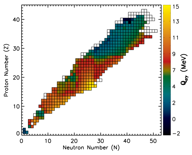
Figure 1: Reaction $Q$ values for the $\mathrm{(\alpha,\gamma)}$ channels within our reference network of 489 isotopes. $Q_{\alpha\gamma}$ is also equivalent to the alpha capture thresholds $S_{\alpha}$. ($N,Z$) boxes correspond to the $Q$ value of reaction ${}^{A}_{Z}{X}(\alpha,\gamma)^{A+4}_{Z+2}{Y}$. White boxes imply the absence of an $\mathrm{(\alpha,\gamma)}$ reaction.

Reaction cross sections have, in general, an asymptotic trend towards a saturation value at high energies. Reactions tend to get balanced by their reverses in this regime. A reaction rate is connected to its reverse according to the detailed balance theorem (Iliadis, 2007). The dominant term in this relationship is $\exp(-Q/kT)$, implying that the reaction $Q$ value and the temperature are the foremost magnitudes related with the ability of a reaction to reach and maintain equilibrium. There is a linear density dependence to this relationship only for reactions involving photons. Large $Q$ values result in sensitive reaction equilibria, which are the first to break for decreasing temperature. However, these reactions become the most efficient flow carriers once they break equilibrium, since they release the largest amounts of energy per reaction. Figure 1 shows the $Q$ value distribution for alpha particle captures within our base network containing 489 isotopes, which includes all reactions that may directly affect $\mathrm{{}^{44}Ti}$. Table 1 gives a complete specification of all networks used in this study.

The temperature expresses the internal energies of the nuclei, while the density is related to their availability for reactions. As a result, the larger the temperatures and densities are, the more equilibria exist. This effect allows NSE to be established for large temperatures and densities. For smaller temperatures and densities, certain equilibria start breaking, but a large scale QSE structure in the plasma may still exist. For yet lower thermodynamic conditions, the large scale clusters dissolve into smaller clusters. Very low temperatures and densities are not adequate to establish a significant amount of equilibria. A few isolated equilibria may exist, but without any specific connection between them. Depending on the initial peak temperature and density, the plasma may experience one or more of these states during the expansion of the ejecta (see Figure 2). Unfortunately, the threshold conditions to border each regime cannot be known accurately, since they are sensitive to the number of species involved (network size), the $Q$ values of the associated reactions and the reaction rates used. Such borders exist in nature though, and the time spent by the plasma in each regime may affect the final yields.

External flow supply to reactions may also result in equilibria breaks, even for constant temperature and density. When there are no external abundance flows to reaction $i(j,k)m$, the condition $\phi_{i}=-\phi_{m}$ means the forward flow for isotope $i$ is the reverse flow for isotope $m$ and vice versa. Due to this condition, this reaction may achieve equilibrium, a case where both $\phi_{i}$ and $\phi_{m}$ are equal to zero. Assume now an external abundance flow, say from another reaction that is not in equilibrium, that supplies flow only to isotope $i$. As long as the external flow is significant in magnitude, $|\phi_{i}|\neq|\phi_{m}|$ because the external flow is additive only to $\phi_{i}$. That is, the external flow term is applied to the equation for $dY_{i}/dt$ but not to the equation for $dY_{m}/dt$, and the reaction $i(j,k)m$ breaks equilibrium. If the external abundance flow is applied long enough, a new equilibrium state may be established. Turning off the external flow causes the reaction to be driven back to equilibrium with a new abundance ratio, depending on the flow transfer by the external agent. In general, starting from an equilibrium state, a transition to any other state means some $|\phi|$’s must be greater than other $|\phi|$’s during the transition. External flows may also affect the equilibrium state of small clusters of nuclei, or even large scale QSE clusters (see §5).

3 Parameterized Thermodynamic Trajectories

We use two parameterized expansion profiles to identify robust trends and uncertainties in the yield of ⁴⁴Ti and ⁵⁶Ni. Both profiles assume that a passing shock wave heats material to a peak temperature $T_{0}$ and compresses the material to a peak density $\rho_{0}$. This material then expands and cools down (freezes out) under the assumption of a constant $T^{3}/\rho$ evolution (radiation entropy in suitable limits) until the temperature and density are reduced to the extent that nuclear reactions cease. Our adiabatic freeze-out trajectories (Hoyle et al., 1964; Fowler & Hoyle, 1964)

$$\frac{dT}{dt}=-\frac{T}{3\tau}\quad\frac{d\rho}{dt}=-\frac{\rho}{\tau}$$ (1)

$$T(t)=T_{0}\exp(-t/3\tau)\quad\rho(t)=\rho_{0}\exp(-t/\tau)$$ (2)

are used with a static free-fall timescale for the expanding ejecta

$$\tau=(24\pi G\rho_{0})^{-1/2}\approx 446/\rho_{0}^{1/2}\ {\rm s}$$ (3)

In this formulation the temperature and density evolutions are decoupled. If one uses $\rho(t)$ in the expansion timescale instead of the peak density $\rho_{0}$, then the temperature ordinary differential equation becomes coupled to the density evolution.

The second thermodynamic profile we use is based on homologous expansion. For a fixed expansion velocity $\upsilon$, the distances increase as $R(t)=R_{0}+\upsilon t$, the density scales as $\rho(t)\sim 1/R(t)^{3}=1/(R_{0}+\upsilon t)^{3}$ and the temperature scales through $\rho\varpropto T^{3}$. Specifically we use

$$\frac{dT}{dt}=\frac{-T_{0}}{1/2(2t+1)^{2}}\quad\frac{d\rho}{dt}=\frac{-3\rho_{0}}{1/2(2t+1)^{4}}$$ (4)

$$T(t)=\frac{T_{0}}{2t+1}\quad\rho(t)=\frac{\rho_{0}}{(2t+1)^{3}}\enskip,$$ (5)

where the coefficients in the denominator are chosen to mimic trajectories taken from core-collapse simulations. Substituting the power-law solution into the ordinary differential equations they originate from and eliminating the direct time dependence

$$\frac{dT}{dt}=-\frac{T_{0}}{0.5(\rho/\rho_{0})^{2/3}}\quad\frac{d\rho}{dt}=-\frac{3\rho_{0}}{0.5(T/T_{0})^{4}}$$ (6)

shows the temperature and density evolutions are coupled for the power-law trajectories.

Figure 2 compares the general properties of these two parameterized profiles. For a given initial condition, the power-law evolution is always slower than the exponential one. Moreover, the power-law evolution becomes slower for increasing initial values. The differences in these two profiles affect the final yields of ⁴⁴Ti and ⁵⁶Ni as material traverses different burning regimes on different timescales. The figure also depicts the NSE, global QSE, local QSE, and final freeze-out burning regimes. The exponential and power-law trajectories are chosen so that they bound in general the temperature and density trajectories of particles from the ⁴⁴Ti and ⁵⁶Ni producing regions of spherically symmetric and 2D explosion models.

For any given peak temperature, peak density, and initial electron fraction $Y_{e}$ we want to know the mass fraction of ⁴⁴Ti and ⁵⁶Ni produced by nuclear burning from the exponential and power-law profiles. We chose peak temperatures, peak densities, and $Y_{e}$ values spanning the range of $4\times 10^{9}\leqslant T_{0}\leqslant 10\times 10^{9}$ K, $10^{4}\leqslant\rho_{0}\leqslant 10^{10}$ g cm^-3, and $0.48\leqslant Y_{e}\leqslant 0.52$. This parameter space covers the conditions encountered in most core-collapse supernova models which produce some ⁴⁴Ti or ⁵⁶Ni. When sampling this parameter space between these limits we use 121 points, equally spaced in base 10 logarithm, for the peak temperature or density and increments of 0.002 in $Y_{e}$. That is, for any value of $Y_{e}$ we compute the final nucleosynthesis at 121x121 points in the peak temperature-density plane using mature reaction networks (Timmes, 1999; Fryxell et al., 2000). Using a larger number of sample points does not alter our main results and conclusions. Our initial composition for any starting ($T_{0}$, $\rho_{0}$, $Y_{e}$) triplet is pure $\mathrm{{}^{28}Si}$ for symmetric matter ($Y_{e}$=0.5). We then added protons or neutrons to make initial composition either proton or neutron-rich respectively. Specifically, we used X(²⁸Si) = 1 - $|$2 $Y_{e}$ - 1$|$ and either X(p) = $|$2 $Y_{e}$ - 1$|$ for proton-rich compositions ($Y_{e}>0.5$) or X(n) = $|$2 $Y_{e}$ - 1$|$ for neutron-rich compositions ($Y_{e}<0.5$) to set the initial ²⁸Si, proton or neutron mass fractions. As we show below in §5, the choice of ²⁸Si is not important for vast regions of the chosen parameter space.

4 Trends in the Peak Temperature-Density Plane

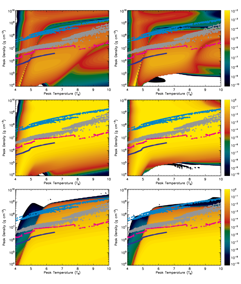
Figure 3: Final mass fraction of ⁴⁴Ti (first row), ⁵⁶Ni (second row) and ⁴He (third row) in the peak temperature-density plane for the exponential thermodynamic profile (first column) and power-law profile (second column) at $Y_{e}$=0.5. Different colored triangles show the temperature-density positions from different supernova and hypernova models - blue for a 1D Cas A model (Young et al., 2006), gray for the 2D rotating progenitor E15B model (Fryer & Heger, 2000), pink for a 1D hypernova model (Fryer et al., 2006), and cyan for a 2D magnetohydrodynamic collapsar model.

Figure 3 shows the mass fractions of ⁴⁴Ti, ⁵⁶Ni and ⁴He produced in the peak temperature-density plane for the exponential and power-law profiles and an initial $Y_{e}$=0.5. Each point in the plane represents one set of initial conditions, which are evolved forward in time according to Equations 1 or 4, with the final freeze-out abundance of ⁴⁴Ti and ⁵⁶Ni recorded. The color map is logarithmic, spanning mass fractions from 10^-2 to 10^-10 for ⁴⁴Ti and from 1 to 10^-10 for ⁵⁶Ni. The overlaid colored triangles correspond to the temperature and density of particles from a suite of supernovae and collapsar simulations in the region where ⁴⁴Ti and ⁵⁶Ni are produced. Not all particles have an initial $Y_{e}$=0.5, but are relatively close to it. Each supernova model generally spans the full range of peak temperature, but the peak density is confined to a strip of one or two orders of magnitude.

Several striking patterns emerge from these contour plots. The first is $\mathrm{{}^{44}Ti}$ seems to be produced overall with an average mass fraction $\mathrm{X(\mathrm{{}^{44}Ti})\sim 10^{-5}}$, except in certain regions where it gets depleted. The depletion region extends along a thin line for low temperatures (oriented approximately $70^{\circ}$ with respect to the temperature axis), smoothly bending over into a wider, more horizontal band for relatively high temperatures and densities. We name this depletion region the “chasm”. The chasm separates the peak temperature-density plane into distinct regions controlled by different burning processes.

The second pattern is that the ⁴⁴Ti contour plots for the two thermodynamic profiles have the same general structure, except that the chasm for the power-law profile is located at lower densities and slightly wider compared to the exponential profile. Hence, the power-law chasm begins to encompass the majority of the overlaid particles. It is possible that the existence of the chasm region is why so few supernova remnants have been observed in the glow of radioactive ⁴⁴Ti. The total mass of $\mathrm{{}^{44}Ti}$ ejected by an individual core-collapse supernova depends critically on (i) the location of its thermodynamic points in the peak temperature-density plane and (ii) the exact expansion profile that the ejecta follow past the explosion. The impact of the latter is expressed as the chasm’s ability to “shift” and “widen” itself from exact profile to exact profile. The third pattern is ⁵⁶Ni has large mass fractions and is relatively featureless in the peak temperature-density plane. Large variations in observed ⁴⁴Ti to ⁵⁶Ni ratios are primarily due to variations in ⁴⁴Ti.

The chasm’s formation and trends with thermodynamic history are the primary motivation for using two parameterized profiles. Our analysis to uncover the nuclear physics controlling the chasm is two-fold. First, we ascertain the basic synthesis mechanisms of $\mathrm{{}^{44}Ti}$ in distinctive thermodynamic regions through a series of nuclear reaction network calculations (section 5). Second, we identify reactions crucial to $\mathrm{{}^{44}Ti}$ in each thermodynamic region via a three-stage process based roughly on the methodology established by The et al. (1998), but modified because we are interested in more than one normalization point in each peak temperature-density plane (section 6).

5 Nucleosynthesis of ⁴⁴Ti and ⁵⁶Ni

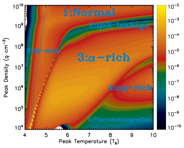
Figure 4: Final mass fraction of ⁴⁴Ti in the peak temperature-density plane for the exponential thermodynamic profile at $Y_{e}$=0.5. Six distinct regions of ⁴⁴Ti synthesis are labeled. Region 1: normal freeze-out from NSE, abundance largely determined from $Q$ values. Region 2: Chasm region, passage from 1 QSE cluster to 2 QSE clusters. Region 3: $\alpha$-rich freeze-out. Region 4: $\alpha$$p$-rich freeze-out. Region 5: Photodisintegration regime, neutrons, protons, and $\alpha$ dominate. Region 6: Incomplete silicon burning, $\mathrm{{}^{28}Si}$ rich. The thin cyan line is the locus of points where $\tau_{{\rm QSE}}$ = 0.012 $\tau_{{\rm freeze}}$.

Figure 4 shows the mass fraction of ⁴⁴Ti in the peak temperature-density plane for the exponential profile and $Y_{e}$=0.5. Each point in this plane represents one set of initial conditions which evolve forward in time with the final freeze-out abundance of ⁴⁴Ti cataloged. Six different regions are labeled which are characterized by specific nuclear burning patterns controlling the production of $\mathrm{{}^{44}Ti}$. Despite the differences in timescale, the corresponding temperature-density contour plot following the power-law profile contains the same number of regions, with similar physics associated between regions of the same label. Thus, the duration of the hydrodynamic expansion does not explain the underlying structure of the contour plots for the final $\mathrm{{}^{44}Ti}$ and $\mathrm{{}^{56}Ni}$ yields. Instead, the entropy during the expansion drives the nucleosynthesis, by affecting the strengths of key nuclear reactions, and causing phase transitions in the burning process for certain critical temperatures and densities. The phase transitions are followed by a change in the burning state. On the other hand, the expansion timescale affects the locus of the borders among different regions on the contour plot (Figure 3). For increasing expansion timescale the plasma spends more time within each burning state. Depending on the region in the peak temperature-density plane, the evolution may include some or all states between NSE and non-equilibrium nuclear burning (see Figure 2). Timescale differences between profiles result in different density values, when the temperature acquires a threshold value indicative of a phase transition. Since both profiles attain constant radiation entropy, different densities at threshold temperatures translate to different peak densities and hence, border shifts between regions on the temperature-density plane (e.g. see §6.3 for the explanation of the chasm shift).

For most of the regions in Figure 4, the peak conditions are sufficiently large that the plasma reaches a large scale equilibrium state (NSE or QSE) on timescales much shorter than the freeze-out timescale. During the first time steps of a reaction network calculation the initial composition rearranges to an NSE or a QSE distribution well before the temperature and density begin evolving. This rapid rearrangement appears as vertical line in many of our plots. As the plasma subsequently cools and rarefies the first transition occurs when the NSE state can no longer be maintained. The threshold temperature for NSE is usually taken to be $T_{9}=T/(10^{9}\ {\rm K})\sim 5$. The density at this threshold temperature determines the subsequent burning process by prescribing both the available amount of nuclear fuel and the dominant flows that consume the fuel.

Region 1 is essentially a freeze-out from NSE, henceforth termed a “normal freeze-out” (Woosley et al., 1973; Meyer, 1994; Meyer et al., 1998; Hix & Thielemann, 1999). When the temperature falls to the $T_{9}=5$ threshold temperature, the density is $\sim$1.0$\times$10⁹ g cm^-3 for the high peak density region above the horizontal band of the chasm. At this density an NSE distribution is dominated by $\mathrm{{}^{56}Ni}$, contains a significant amount of Si-group and Fe-group nuclei, but a relatively small amount of free alpha particles ($\mathrm{X_{\alpha}\sim 10^{-3}}$). This density is large enough to favor particle captures, but the temperature is such that photodisintegration reactions are not negligible either. The large scale equilibrium structure is maintained until complete freeze-out, since $\mathrm{X_{\alpha}\ll 1}$ for the majority of equilibrium states and the 3$\alpha$ reaction is always dominated by its inverse photodisintegration. Since normal freeze-out is a dynamic process though, some individual equilibria are broken as the plasma cools and rarefies and QSE estimates become progressively more accurate compared to NSE estimates (Woosley et al., 1973). Yields for the isotopes plotted in Figure 5 for region 1 (first row of plots) are not far from NSE or QSE yields. Thus, network calculations in this region may be avoided and accurate estimates for yields may be determined only by nuclear properties such as masses and $Q$ values.

Equilibrium estimates for Si-group and Fe-group nuclei during the initial stages of the expansion remain relevant for region 2. When the temperature falls to the $T_{9}=5$ threshold temperature the density is $\sim$1.0$\times$10⁸ g cm^-3. The low availability of alpha particles at this density does not allow the 3$\alpha$ reaction to dominate its inverse, preventing significant flow from the light nuclei to the equilibrium cluster. Compared to region 1 though, not all of the capture reactions have the same efficiency. The large $\alpha$ thresholds in nuclei between N,Z=20 and N,Z=26 closed shell configurations results in a phase transition which is responsible for the formation of the chasm. Because of the large $Q$ values associated with $\alpha$ capture in the mass range $42\leqslant A\leqslant 53$ due to shell structure (Figure 1), these reactions are the first to break the local equilibria and form a continuous passage of nuclear flow from the Si-Ca-group to the Fe-group nuclei. The large equilibrium cluster dissolves into two smaller ones, with $\mathrm{{}^{44}Ti}$ being located within the upper mass limits of the Si-Ca cluster, while $\mathrm{{}^{56}Ni}$ is centralized in the Fe-group. The flow transfer between the two equilibrium clusters results in the depletion of $\mathrm{{}^{44}Ti}$ and the rest of the isotopes in the Si-group by the end of the thermodynamic evolution (second row of Figure 5). On the contrary, $\mathrm{{}^{56}Ni}$ is one of the Fe-group isotopes that benefit from this transfer since the reaction equilibria in its neighborhood are maintained until freeze-out. Equilibria estimates for this small group of nuclei within the Fe-group are still a good approximation. The formation of the chasm in Figure 4 is a direct result of a phase transition from the single cluster QSE configuration to a double cluster QSE configuration and the subsequent flow leakage.

Region 3 corresponds to the conditions of $\alpha$-rich freeze-out (Woosley et al., 1973). As the plasma cools and rarefies, most Si-group and Fe-group mass fractions acquire the topology of an “arc” in going from low values at high temperatures to a local maximum and back to a local minimum at cooler temperatures, while in QSE (third row of Figure 5). The density at the $T_{9}$=5 threshold temperature within region 3 spans $10^{4}\lesssim\rho\lesssim 10^{7}$ g cm^-3, resulting in less efficient particle captures compared to regions 1 and 2, and a helium mass fraction $\mathrm{X_{\alpha}\sim 10^{-1}}$. The excess of free alpha particles allows the $3\alpha$ rate to dominate its inverse photodisintegration, leading to a new phase transition. Although the $3\alpha$ rate remains relatively slow (The et al., 1998), it supplies external flow which breaks the local equilibria in the neighborhood of $\mathrm{{}^{12}C}$, $\mathrm{{}^{16}O}$ and $\mathrm{{}^{24}Mg}$. The subsequent energy release from alpha capture reactions provides a significant nuclear flow towards heavier nuclei by breaking successively other local equilibria. The QSE cluster changes its shape and shifts gradually upwards in mass, instead of dissolving into two clusters. Meyer et al. (1998) identified this cluster motion based on QSE calculations. The mass fractions of nuclei which suddenly find themselves outside the QSE cluster begin an ascending track. These are primarily the Si-group nuclei (including $\mathrm{{}^{44}Ti}$), and a few from the Fe-group. Close to complete freeze-out, the yields for these nuclei are orders of magnitude larger than their corresponding minimum value reached prior to the phase transition. Because the $3\alpha$ reaction itself is not very efficient, the process ends up with an excess of alpha particles $\mathrm{X_{\alpha}\sim 10^{-2}}$.

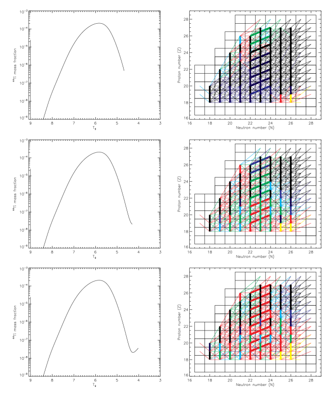
Figure 6: Normalized nuclear flows at three different points in the evolution of ⁴⁴Ti from freeze-out; before the minimum (top panel), at the minimum (middle panel), and after the minimum (bottom panel). Normalized flows $\phi$ are colored black for $0\leq\phi<0.01$, navy for $0.01\leq\phi<0.05$, blue for $0.05\leq\phi<0.1$, cyan for $0.1\leq\phi<0.4$, green for $0.4\leq\phi<0.8$, red for $0.8\leq\phi<1.0$, yellow for $\phi$=1.0. Normalized flows in the vertical direction, corresponding to $(p,\gamma)$ reactions, and along diagonal directions corresponding to $(\alpha,p)$ reactions have been drawn thicker for clarity.

Large scale QSE calculations cannot account for the increase of the $\mathrm{{}^{44}Ti}$ mass fraction curve past the arc, since $\mathrm{{}^{44}Ti}$ and other related isotopes have decoupled from the large scale equilibrium cluster. However, the phase transition is not abrupt in shifting from total equilibrium to total non-equilibrium. Nuclear flow analysis shows that $\mathrm{{}^{44}Ti}$ participates in a smaller, local equilibrium pattern which is responsible for its ascending trend in the mass fraction curve at the end of freeze-out. This transition is demonstrated in Figure 6 which displays the reaction links between f_7/2-shell nuclei located between the Z,N=20 and Z,N=28 closed shells. The top panel in Figure 6 shows the network of reactions prior to the ⁴⁴Ti abundance minimum, which is characterized by $\mathrm{(p,\gamma)}$ equilibria along the N=22 and N=24 isotone chains connected by $\mathrm{(\alpha,p)}$ and $\mathrm{(\alpha,\gamma)}$ channels in equilibrium. These equilibria guarantee linkage of $\mathrm{{}^{44}Ti}$ to the large scale QSE cluster, and hence, the downward portion of the mass fraction curve is produced. The breakdown of the equilibrium conditions for the $\mathrm{\mathrm{{}^{44}Ti}(\alpha,p)\mathrm{{}^{47}V}}$ link signals the phase transition for $\mathrm{{}^{44}Ti}$. Soon afterward, the rest of the $\mathrm{(\alpha,p)}$ and $\mathrm{(\alpha,\gamma)}$ equilibria connecting the N=22 and N=24 isotone chains break, as reflected in the increase of actual net flow shown in the middle panel in Figure 6. $\mathrm{{}^{44}Ti}$ is left in $\mathrm{(p,\gamma)}$ equilibria along the N=22 isotone chain with ⁴⁵V, ⁴⁶Cr, ⁴⁷Mn and ⁴⁸Fe and its mass fraction starts to increase from the local minimum (bottom panel of Figure 6). It is this $\mathrm{(p,\gamma)}$ equilibria chain which is responsible for the rising portion of the mass fraction curve after the local minimum. This pattern persists until complete freeze-out.

These reaction network flow study results can be verified by localized QSE calculations. The advantage of QSE modeling is that the abundances of all isotopes within a cluster may be expressed by a semi-analytical formalism, in terms of the network abundances of free protons, neutrons and an arbitrarily chosen reference isotope. For this purpose, we adopt the Hix & Thielemann (1996, 1999) formalism. We model the cases of equilibrium (i) between the N=22 and N=24 isotone chains and (ii) only along the N=22 isotone chain throughout the evolution, corresponding to the top and bottom panels in Figure 6 respectively. Both cases reproduce the arc topology of the ⁴⁴Ti mass fraction curve. However, the first case does not reproduce the ascending part of the curve beyond the local minimum in Figure 7. Instead, the ⁴⁴Ti curve continues to descend, expressing the trend of $\mathrm{{}^{44}Ti}$, were it to remain in global QSE. The second case on the other hand, which expresses only $(p,\gamma)$ equilibria, fits the network results until the point where complete freeze-out occurs. The discrepancy beyond this point relies on the fact that nuclear reactions no longer take place. Thus, mass fractions do not change any more and the curve from network calculations acquires a plateau. This general behavior applies to most of the elements within the silicon and iron groups, as demonstrated for a small subset within these groups at the upper right panel in Figure 7. The mass fraction trends of an isotope depend strongly on the local reaction equilibria within its neighborhood. Further equilibria isotone chains are readily identifiable in Figure 6. For example, crucial equilibria reactions for $\mathrm{{}^{40}Ca}$ are $\mathrm{\mathrm{{}^{40}Ca}(\alpha,\gamma)\mathrm{{}^{44}Ti}}$ and $\mathrm{\mathrm{{}^{43}Sc}(p,\gamma)\mathrm{{}^{44}Ti}}$. Its mass fraction profile in the lower left of Figure 7 is in accordance with the general mechanism. The increase of the $\mathrm{{}^{40}Ca}$ mass fraction with cooling is maintained through the $\mathrm{(p,\gamma)}$ equilibria along the N=20 isotone chain. A similar development can be observed for $\mathrm{{}^{48}Cr}$ as shown in the lower right of Figure 7, the crucial reaction now is $\mathrm{\mathrm{{}^{48}Cr}(\alpha,p)\mathrm{{}^{51}Mn}}$.

Region 4 is a special case of an $\alpha$-rich freeze-out. Within this region, the $\mathrm{p(e^{-},\nu_{e})n}$ and $\mathrm{n(e^{+},\overline{\nu_{e}})p}$ reactions exert a greater influence compared to the other regions. These reactions drive the composition slightly proton-rich near the beginning of the evolution when temperature and density are still large. Impacts to the burning processes for proton-rich composition are described in more detail in §5.1, but some of the impacts include a relatively high number of free protons and an enhanced efficiency of proton captures (Pruet et al., 2005, 2006; Buras et al., 2006; Fröhlich et al., 2006). Consequently, this region is a proton-rich, $\alpha$-rich freeze-out, henceforth an “$\alpha$$p$-rich freeze-out”. The fourth row of Figure 5 shows the mass fraction profiles for $\mathrm{{}^{44}Ti}$ in region 4 have certain similarities to the profiles in region 3. A characteristic arc of large scale QSE is formed, followed by the ascending track due to the equilibrium chain connecting $\mathrm{{}^{44}Ti}$, $\mathrm{{}^{45}V}$, $\mathrm{{}^{46}Cr}$, $\mathrm{{}^{47}Mn}$ and $\mathrm{{}^{48}Fe}$ via $\mathrm{(p,\gamma)}$ reactions along the N=22 isotone chain. Among these linking reactions $\mathrm{\mathrm{{}^{45}V}(p,\gamma)\mathrm{{}^{46}Cr}}$ has the largest $Q$ value, and thus will break its equilibrium first as the plasma cools and rarefies. When this reaction breaks equilibrium, the N=22 isotone chain dissolves into two smaller clusters, the first between $\mathrm{{}^{44}Ti}$ and $\mathrm{{}^{45}V}$ and a second between $\mathrm{{}^{46}Cr}$, $\mathrm{{}^{47}Mn}$ and $\mathrm{{}^{48}Fe}$. This is the second phase transition that $\mathrm{{}^{44}Ti}$ sustains during its evolution. Similar transitions occur along other isotone chains. Flows are now carried among such isolated small scale clusters by out of equilibrium alpha and proton captures. These flows favor mostly the proton-rich nuclei, resulting in a decrease for $\mathrm{{}^{44}Ti}$ and other symmetric isotopes. Thus, a second arc is clearly identifiable in the mass fraction curve for most of the isotopes in the fourth row of Figure 5. The ascending track beyond the second arc for $\mathrm{{}^{44}Ti}$ and most of the symmetric isotopes is a consequence of the flow transfer through weak interactions at the expense of proton-rich nuclei, when the strong and electromagnetic reactions become ineffective as freeze-out takes place.

In region 5 the temperatures are initially large enough to establish equilibrium (NSE or QSE), but the initial densities are so low that photodisintegrations soon dominate capture reactions. Long before the complete freeze-out, all nuclei dissolve into neutrons, protons and $\alpha$-particles. A slight recombination takes place during the final stages of the freeze-out producing traces of $\mathrm{{}^{12}C}$, $\mathrm{{}^{16}O}$ and $\mathrm{{}^{28}Si}$. The recombination is driven mostly by the 3$\alpha$, $\mathrm{p(e^{-},\nu_{e})n}$ and $\mathrm{n(e^{+},\overline{\nu_{e}})p}$ reactions in $Y_{e}\geqslant 0.5$ matter. The products of this recombination set the seed for a following chain of $\mathrm{(p,\gamma)}$ and $\mathrm{(n,p)}$ reactions that produce heavier elements, including $\mathrm{{}^{44}Ti}$, $\mathrm{{}^{56}Ni}$ and the heaviest isotopes in the network used for the calculation. Similarly to region 4, weak interactions at the close of the process carry some flow from proton-rich nuclei to symmetric ones, enhancing this way the mass fractions of $\mathrm{{}^{44}Ti}$ and $\mathrm{{}^{56}Ni}$. However, the contributions of the recombination and the chain of $\mathrm{(p,\gamma)}$ and $\mathrm{(n,p)}$ reactions are not adequate to yield large production factors for most of the isotopes. The final composition is dominated by free alpha particles and protons, establishing this region to be a photodisintegration driven regime.

Region 6 represents incomplete silicon burning, where $\mathrm{{}^{28}Si}$ gradually dominates $\mathrm{{}^{56}Ni}$ from region 1 to the left of the thin chasm line towards the inner part of this region. The peak temperatures and densities are such that the timescale to reach a single cluster QSE state is comparable or larger than the expansion timescale. Multiple small scale QSE clusters are formed, but they do not merge successfully into one large scale cluster. The mass fractions freeze out from the established equilibrium state without sustaining any phase transition. This resembles the mass fraction trends within region 1, only that the freeze-out within region 6 originates from equilibria states which are sensitive to the number and shape of clusters formed, and thus from the initial composition for the burning process. The physical border between regions 3 and 1 is the thin chasm line oriented $\sim 70^{\circ}$ with respect to the peak temperature axis. Such a distinctive border does not exist between regions 1 and 6, due to the lack of a phase transition in both regions. However, an approximate border is the locus of points given by $\tau_{{\rm QSE}}$ = 0.012 $\tau_{{\rm freeze}}$, where $\tau_{{\rm QSE}}$ is the timescale to reach QSE (Calder et al., 2007) and $\tau_{{\rm freeze}}$ is given by equation 3. This locus is shown by the thin cyan line in Figure 4. The relative differences for $\mathrm{{}^{44}Ti}$ yields starting from pure $\mathrm{{}^{28}Si}$ or $\mathrm{{}^{12}C}$ are less than 0.1 to the right of this locus.

The case of $\mathrm{{}^{56}Ni}$ is simpler than $\mathrm{{}^{44}Ti}$. The isotope $\mathrm{{}^{56}Ni}$ tends to dominate the final composition for the majority of the peak temperatures and peak densities for $Y_{e}=0.5$. The topology of its final mass fractions in Figure 3 shows $\mathrm{{}^{56}Ni}$ does not sustain any phase transitions like $\mathrm{{}^{44}Ti}$ because $\mathrm{{}^{56}Ni}$ remains in equilibrium with its local neighborhood (Woosley & Hoffman, 1992). While the macroscopic behavior of the large QSE cluster changes in different regions, there are almost no changes in $\mathrm{{}^{56}Ni}$.

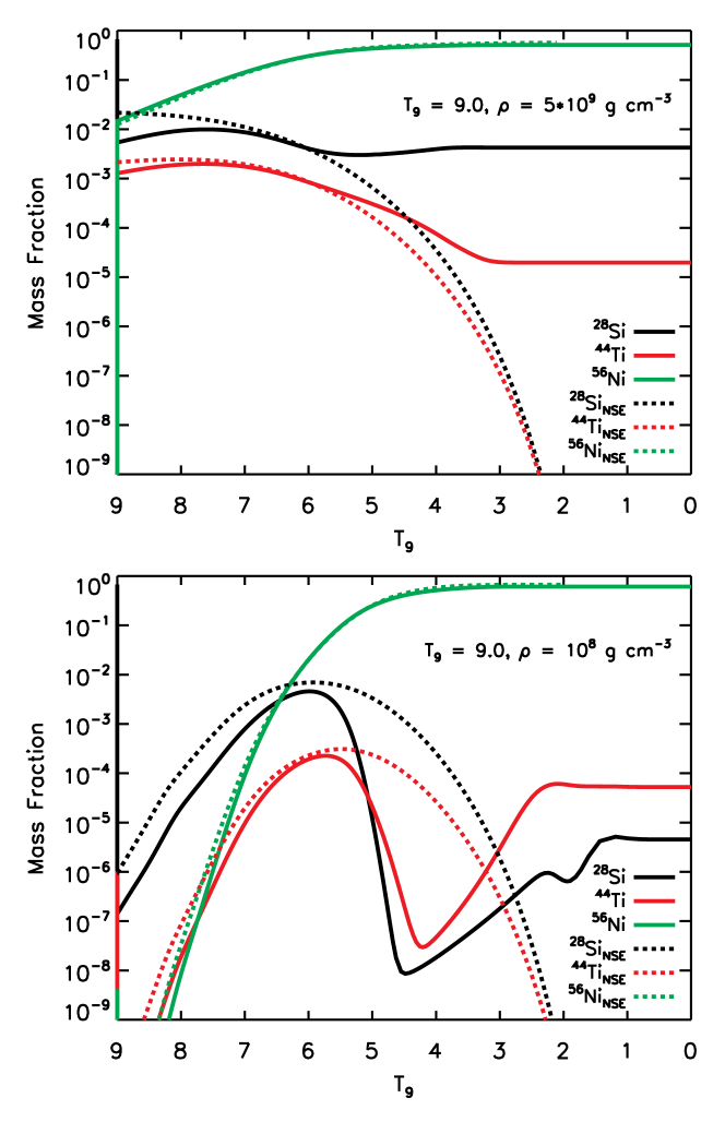
Figure 8: Mass fraction evolution of key isotopes from network and NSE calculations for peak temperatures and peak densities corresponding to a normal freeze-out (top panel) and an $\alpha$-rich freeze-out (bottom panel).

In region 1, a single QSE cluster which includes ⁵⁶Ni stays intact until freeze-out. In region 2, the QSE cluster dissolves into two smaller ones, with the cluster localized around the Fe-group nuclei encompassing $\mathrm{{}^{56}Ni}$ at all times. During the $\alpha$-rich freeze-out of region 3 the QSE cluster shifts upwards in mass and shrinks (Meyer et al., 1998), but remains centralized on Fe-group nuclei (including $\mathrm{{}^{56}Ni}$). Near the end of the evolution, the Fe-group nuclei are the most abundant in the network with reaction equilibria maintained among them. Figure 8 shows the mass fractions of $\mathrm{{}^{28}Si}$, $\mathrm{{}^{44}Ti}$ and $\mathrm{{}^{56}Ni}$ for a normal and an $\alpha$-rich freeze-out, accompanied by the corresponding NSE values for each isotope were the NSE valid at all times. For the normal freeze-out, the network values are in good agreement with the corresponding NSE values until the NSE threshold of $T_{9}\sim$5. For $\mathrm{{}^{56}Ni}$, the agreement between the network and NSE values persists until at least $T_{9}\sim$2, at which point our NSE solver fails to converge. During an $\alpha$-rich freeze-out the network values of $\mathrm{{}^{28}Si}$ and $\mathrm{{}^{44}Ti}$ are quite different from their corresponding assumed NSE values, while the NSE mass fraction of $\mathrm{{}^{56}Ni}$ still agrees with reaction network values until $T_{9}\sim$2. Of course NSE at $T_{9}\sim$2 does not exist, but the trends in Figure 8 suggest that $\mathrm{{}^{56}Ni}$ may be considered to be in a large scale equilibrium throughout the evolution for almost every region on the temperature-density plane. That is, global equilibrium estimates may interpret adequately the dominant trend of $\mathrm{{}^{56}Ni}$ for an initially symmetric composition.

5.1 Electron fraction sensitivity study

The electron fraction, or the total proton to nucleon ratio, $Y_{e}=\sum_{i}Z_{i}Y_{i}=\sum_{i}\frac{Z_{i}}{A_{i}}X_{i}$ , is equivalent to a weighted average of isotopic proton to nucleon ratios, where each has a probability equal to $X_{i}$. Since the distribution of isotopic ratios in a large network may be approximated as continuous, the most abundant isotopes at any given time in the thermodynamic evolution are generally the ones whose individual proton to nucleon ratio is within a small range from the current value of the electron fraction. A small spread usually exists due to nuclear structure effects for equilibrium states (expressed primarily with $Q$ values), and reaction rate values for non-equilibrium states (Arnett, 1977). The largest (major) nuclear flows tend to be localized along the most abundant nuclei, since the flows depend on multiplications of abundances. During NSE or QSE the major flows result in the most robust reaction equilibria, while the same reactions typically become the most efficient carriers of nuclear flow as soon as they depart from equilibrium. Almost all our $Y_{e}$ sensitivity results may be explained by these guidelines for the major flows. An exception exists for cases with initial $Y_{e}>0.5$ during large scale equilibrium (NSE and QSE), where the equilibrium patterns are configured according to a different principle (Seitenzahl et al., 2008). Electron fraction variations alter the nuclear composition and affect the yields, the nucleosynthesis mechanisms for each region in the peak temperature-density plane, and change the regions topology.

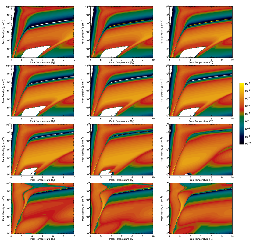
Figure 9: Final yield of ⁴⁴Ti in the peak temperature-density plane for different values of the initial electron fraction $Y_{e}$ under the exponential freeze-out profile. The top row, from left to right, corresponds to $Y_{e}$ = 0.484, 0.486, and 0.488. The second row, from left to right, corresponds to $Y_{e}$ = 0.490, 0.492, and 0.494. The third row, from left to right, corresponds to $Y_{e}$ = 0.496, 0.498, and 0.500. The bottom row, from left to right, corresponds to $Y_{e}$ = 0.502, 0.504, and 0.506.

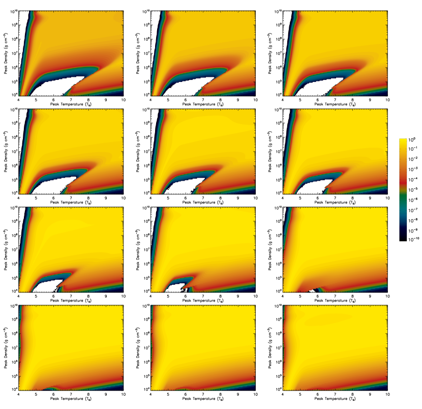
Figure 10: Same as Figure 9, but for the final yield of ⁵⁶Ni.

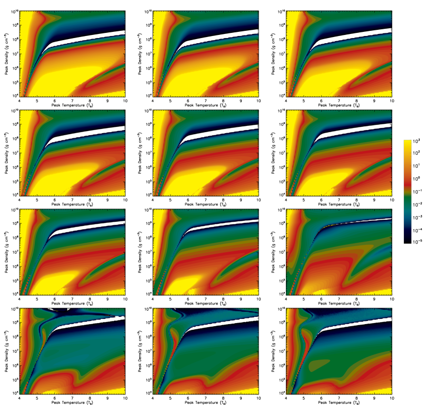
Figure 11: Same as Figure 9, but for the $\mathrm{{}^{44}Ti}$ normalized production factor P₄₄.

Figures 9 and 10 show the final yields of ⁴⁴Ti and ⁵⁶Ni, respectively, in the peak temperature-density plane for $0.484\leqslant Y_{e}\leqslant 0.506$ under the exponential freeze-out profile. Figure 11 shows the ⁴⁴Ti production factor P₄₄ for the same range of $Y_{e}$. The production factor for a given species is defined as the final mass fraction of the species in question divided by the mass fraction to which it decays in the Sun. These production factors are then normalized to the production factor of ⁵⁶Fe (Woosley & Hoffman, 1991; Hoffman et al., 2010). Within the electron fraction values 0.498 and 0.5, yields for both isotopes are maximized, resulting to the minimization of the chasm’s width and depth for $\mathrm{{}^{44}Ti}$. For decreasing $Y_{e}$ values, both isotopes tend to be under-produced compared to the symmetric case (Woosley & Hoffman, 1992). For increasing $Y_{e}$ values, $\mathrm{{}^{56}Ni}$ is still favored by equilibria schemes and is produced at an amount comparable to the symmetric case (Magkotsios et al., 2008). The temperature-density planes for $\mathrm{{}^{56}Ni}$ have similar featureless structure to the corresponding plane for initially symmetric matter, implying that this isotope is produced only by equilibria schemes without sustaining any phase transition. The location of the border between the regions of $\alpha$-rich and $\alpha$$p$-rich freeze-out for $\mathrm{{}^{44}Ti}$ depends on the initial electron fraction value. The lack of free protons for neutron-rich environments favors the $\alpha$-rich freeze-out versus the $\alpha$$p$-rich one, until the $\alpha$$p$-rich freeze-out is not manifested at all for $Y_{e}\approx 0.46$. The situation is gradually reverted for increasing $Y_{e}$, until the $\alpha$$p$-rich freeze-out dominates the $\alpha$-rich freeze-out for $Y_{e}\approx 0.506$. These trends are in accordance with the major flows guidelines discussed above, since both isotopes are symmetric with an individual proton to nucleon ratio equal to 0.5, and the amount of free protons increases significantly for $Y_{e}>0.5$ (Seitenzahl et al., 2008). Further changes to the topological structure compared to the symmetric case include the appearance of a depletion region for both $\mathrm{{}^{44}Ti}$ and $\mathrm{{}^{56}Ni}$ for decreasing $Y_{e}$, and the appearance of a physical border between regions 1 and 6 for increasing $Y_{e}$. This physical border implies a new type of phase transition that $\mathrm{{}^{44}Ti}$ sustains. These trends are the same for the power-law freeze-out profile (not shown).

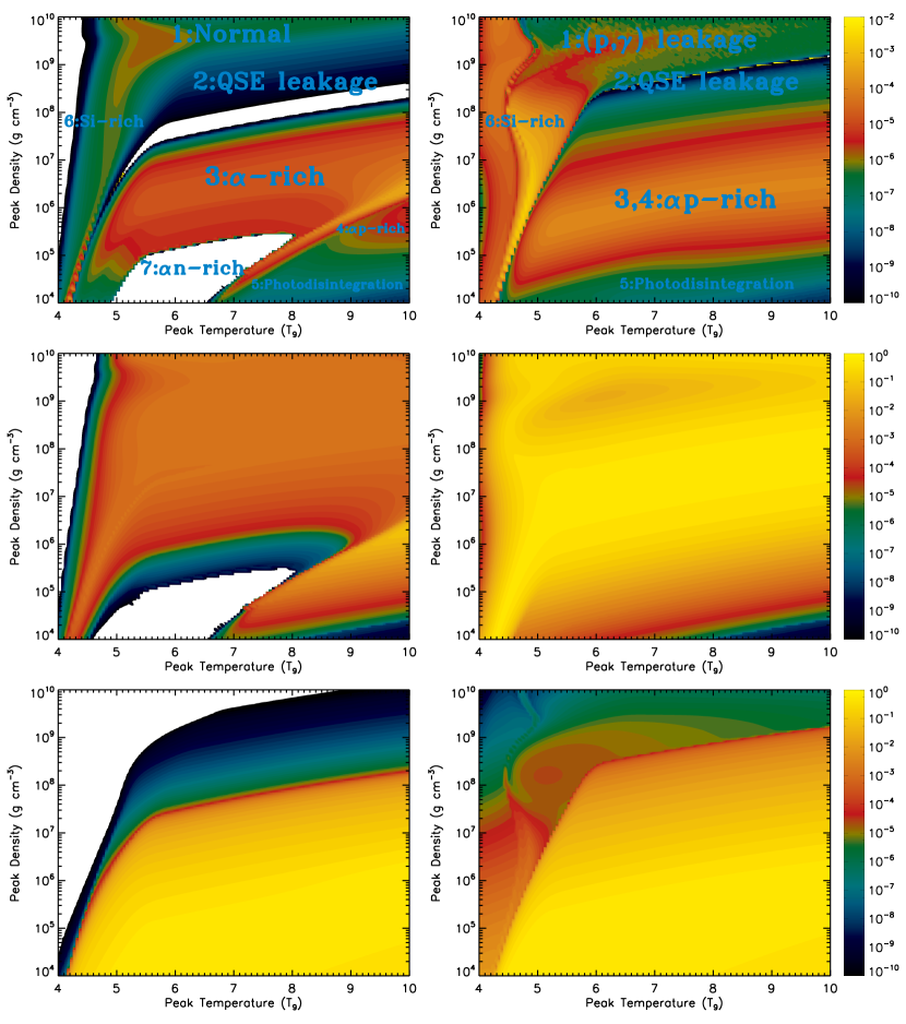
Figure 12: Final mass fraction of ⁴⁴Ti (first row), ⁵⁶Ni (second row) and ⁴He (third row) in the peak temperature-density plane for the exponential thermodynamic profile at $Y_{e}$=0.48 (left column) and $Y_{e}$=0.52 (right column). The distinct regions of ⁴⁴Ti synthesis are labeled. Region 1: normal freeze-out from NSE (left), (p,$\gamma$) leakage from symmetric to proton-rich nuclei (right). Region 2: Chasm region, passage from 1 QSE cluster to 2 QSE clusters. Region 3: $\alpha$-rich freeze-out. Region 4: $\alpha$$p$-rich freeze-out. Region 5: Photodisintegration regime, neutrons, protons, and $\alpha$ dominate. Region 6: Incomplete silicon burning, $\mathrm{{}^{28}Si}$ rich. Region 7: $\alpha$$n$-rich freeze-out.

We focus next on two relatively extreme $Y_{e}$ values, 0.48 for the neutron-rich case and 0.52 for the proton-rich one. Both values are adequately far from the standard value of symmetric matter, so that the differences in the trends for ⁴⁴Ti and ⁵⁶Ni are emphasized and easily identified. The characteristic regions of the $\mathrm{{}^{44}Ti}$ temperature-density planes with initial electron fraction $Y_{e}$=0.48 and $Y_{e}$=0.52 are labeled in Figure 12 for the exponential profile. Similarly to Figure 4, the only region sensitive to the initial composition is region 6, the incomplete Si-burning regime.

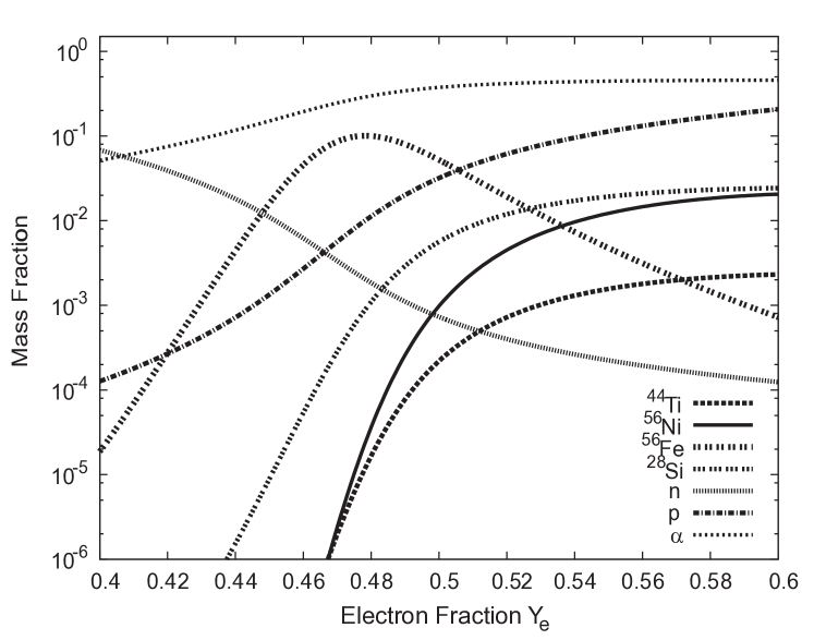
Figure 13: Mass fraction of select isotopes in NSE at $T_{9}=9$ and $\rho=10^{9}$ g cm^-3 for different electron fractions.

For $Y_{e}$=0.48, NSE and QSE favor the formation of nuclei with a proton to nucleon ratio around 0.48 during equilibrium, and the major flows are localized in the neighborhood of the same nuclei during the non-equilibrium parts of the evolution. Despite $\mathrm{{}^{56}Ni}$ being marginally within the range of major flows, large scale equilibrium patterns gradually favor $\mathrm{{}^{56}Fe}$ instead of $\mathrm{{}^{56}Ni}$ for decreasing electron fraction (see Figure 13). Regions 1-6 each have the same type of physics compared to the corresponding ones for initially symmetric matter. The chasm widening is an outcome of the overall underproduction of $\mathrm{{}^{44}Ti}$. The large scale equilibria patterns do not favor $\mathrm{{}^{44}Ti}$ production (see Figure 13), and the normal freeze-out region merges with the chasm. The $\alpha$-rich freeze-out yields less $\mathrm{{}^{44}Ti}$ compared to the symmetric case, ceding additional area to the chasm region. The decreased efficiency of the $\alpha$-rich freeze-out regarding $\mathrm{{}^{44}Ti}$ production is related to the manner that the electron fraction value affects the flow transfer by $\mathrm{(\alpha,\gamma)}$ reactions towards the $N=22$ isotone chain, and the favor of the isotone chains towards neutron-rich isotopes rather than $\mathrm{{}^{44}Ti}$. The size reduction of the $\alpha$$p$-rich freeze-out region is due to the absence of free protons in neutron-rich equilibrium configurations.

Region 7 represents the case of neutron-rich, $\alpha$-rich freeze-out, which barely appears for $Y_{e}$=0.5 (not labeled in Figure 4). It is also known in the literature as the “$\alpha$-process” (Woosley & Hoffman, 1992), but we term it henceforth as “$\alpha$$n$-rich freeze-out”. This region combines the physics of regions 3 and 5. A photodisintegration regime is established early in the evolution and during the equilibrium stages, but contrary to region 5, $\mathrm{p(e^{-},\nu_{e})n}$ and $\mathrm{n(e^{+},\overline{\nu_{e}})p}$ tend to balance each other after the phase transition imparted by the 3$\alpha$ forward rate dominance over its inverse. Thus, the electron fraction value is maintained close to its initial value, well below 0.5. Such values of the electron fraction are prerequisite for the production of elements beyond the Fe-group. Although the electron fraction has similar values within region 3, there are traces of Si-group and Fe-group nuclei during the equilibrium stages. The presence of $\mathrm{{}^{56}Ni}$ blocks the flows towards heavier nuclei during the non-equilibrium stage and neutrons are consumed among the Si-group and Fe-group. However, these traces are absent for the equilibrium stages within region 7, and heavier elements are produced during the non-equilibrium stage. Table 2 lists the dominant yields from freeze-outs for $Y_{e}$ = 0.48, 0.50, and 0.52. The yields from the $\alpha$-rich freeze-out are quite similar for $Y_{e}$ = 0.48 and 0.50 (Woosley & Hoffman, 1992). Since the region for the $\alpha$$n$-rich freeze-out increases in size for decreasing $Y_{e}$, it is expected at some point to dominate all the area enclosed by the chasm.

For $Y_{e}$=0.52, NSE and large scale QSE are dominated by $\mathrm{{}^{56}Ni}$ and free protons, with non-negligible abundances for symmetric and proton-rich nuclei (also see Figure 13), in accordance with a minimum of the Helmholtz free energy. Despite the excess of free protons favored by large scale equilibria patterns, neutrons are captured more efficiently in a proton-rich environment. Thus, $\mathrm{n(e^{+},\overline{\nu_{e}})p}$ reaction dominates $\mathrm{p(e^{-},\nu_{e})n}$, resulting in a slight increase to the value of the electron fraction early in the evolution for the $\alpha$$p$-rich freeze-out region. Since these reaction channels retain $Y_{e}>0.5$ during large scale equilibrium, major flows favor proton-rich nuclei as soon as the QSE cluster dissolves. Thus, for regions 1-5 where NSE and large scale QSE are established, the $\mathrm{(p,\gamma)}$ reactions are all directed towards transferring the flow from symmetric to proton-rich isotopes, which is equivalent to a phase transition that all isotopes in the network sustain. Consequently, there cannot be a normal freeze-out in region 1 (Figure 12), because the freeze-out does not take place from NSE (or large scale QSE). During the non-equilibrium part of the freeze-out evolution, the weak interactions decrease $Y_{e}$ by transferring flow towards more stable isotopes, resulting in its non-monotonic evolution and the reassemble of symmetric isotopes like $\mathrm{{}^{44}Ti}$.

Within the $\alpha$$p$-rich freeze-out region (region 4 in Figure 12) the $\mathrm{{}^{44}Ti}$ mass fraction pattern resembles the corresponding one with initial $Y_{e}=0.5$, with two arcs and an ascending track at the end. A timescale dependent third arc is identifiable for the power-law profile only. Its appearance relies on the equilibrium state of the remaining $\mathrm{{}^{44}Ti}$-$\mathrm{{}^{45}V}$ cluster and the net flow towards this cluster by the interplay between neighboring $\mathrm{(p,\gamma)}$ and weak reactions. $\mathrm{\mathrm{{}^{45}V}(p,\gamma)\mathrm{{}^{46}Cr}}$ is the primary reaction to control the flow leakage off this cluster.

Within region 6, the initially formed small scale QSE clusters fail to merge to a large-scale cluster. This results in randomly directed flow supply among the small scale clusters and the absence of a phase transition accompanied by complete consumption of fuel nuclei. The physical border between regions 1 and 6 is an outcome of the existence of a transition within region 1. For regions 1-5 the final composition is always proton-rich.

6 Reaction rate sensitivities

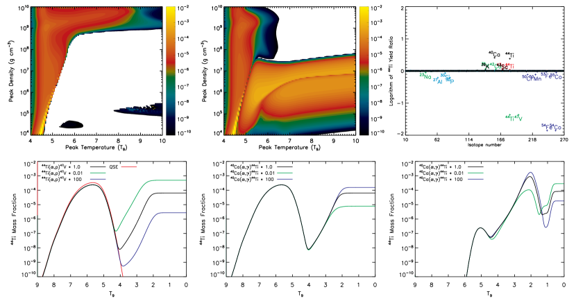
Figure 14: Examples of ⁴⁴Ti sensitivity to reaction rates for the power-law thermodynamic profile at $Y_{e}$=0.5. From left to right in the first row, the contour plots show the effects of removing the 3$\alpha$ and increasing the $\mathrm{p(e^{-},\nu_{e})n}$ + $\mathrm{n(e^{+},\overline{\nu_{e}})p}$ by 1000, while the third plot shows the ratio of the $\mathrm{{}^{44}Ti}$ yield with single rates increased by 100 to the nominal $\mathrm{{}^{44}Ti}$ yield during $\alpha$-rich freeze-out. Isotopes whose reaction rates produce interesting variations are labeled. Black color is used for the ($\alpha$,$\gamma$) reactions, green for the ($\alpha$,p) reactions, red for (p,$\gamma$) reactions, cyan for ($\alpha$,n), and blue for the weak reactions. The second row shows from left to right the $\mathrm{{}^{44}Ti}$ mass fraction sensitivity to $\mathrm{\mathrm{{}^{44}Ti}(\alpha,p)\mathrm{{}^{47}V}}$ and $\mathrm{\mathrm{{}^{40}Ca}(\alpha,\gamma)\mathrm{{}^{44}Ti}}$ for the $\alpha$-rich freeze-out, and $\mathrm{\mathrm{{}^{40}Ca}(\alpha,\gamma)\mathrm{{}^{44}Ti}}$ for the $\alpha$$p$-rich freeze-out. Black curves are for the nominal rates, red curves are for the QSE yields, green curves for rates multiplied by 0.01 and blue curves for rates multiplied by 100.

The topology of the $\mathrm{{}^{44}Ti}$ and $\mathrm{{}^{56}Ni}$ contour plots is affected by certain key reactions, in combination with the timescale of the expansion. We follow a three-stage method to uncover the role and impact of these reactions. Figure 14 exemplifies the three stages of this method. During the first stage, specific reaction channels are either altered or removed from the network calculations for all isotopes (e.g., all $(\alpha,\gamma)$ reactions) to assess the most significant channels for every region. In addition, the $3\alpha$, $\mathrm{p(e^{-},\nu_{e})n}$ and $\mathrm{n(e^{+},\overline{\nu_{e}})p}$ reactions have their own brevet, since they may affect the reaction flows globally (first row in Figure 14). Thus, the term “weak reactions” will imply all such reactions henceforth, excluding $\mathrm{p(e^{-},\nu_{e})n}$ and $\mathrm{n(e^{+},\overline{\nu_{e}})p}$. We tabulate weak reactions by their dominant decay mode, although all decay modes are considered in our calculations. The second stage performs a sensitivity analysis on all groups of reactions by increasing and decreasing reaction rates excessively one at a time (third panel within first row in Figure 14). Similarly to The et al. (1998), reaction rates are either multiplied or divided by a factor of 100. The exception are the weak reactions, where the factor is 1000. The third stage conducts detailed nuclear flows and mass fraction profile analysis to illustrate the impact of the final crucial reactions that affect $\mathrm{{}^{44}Ti}$ (second row in Figure 14). Note the second and third stages are applied independently for every distinctive thermodynamic region in the temperature-density plane. The rates used for our calculations are from the Rauscher & Thielemann (2000) compilation, updated with some experimentally measured rates. Table 3 lists the most important reactions which our sensitivity study has revealed to impact $\mathrm{{}^{44}Ti}$. We rank reactions as “primary” or “secondary”, depending on the differences between the $\mathrm{{}^{44}Ti}$ mass fraction curves for nominal and modified rates. A reaction which involves differences at any point of the evolution by a factor of 10 or larger is ranked primary (Figure 14). Reactions resulting in changes smaller than a factor of 10 are ranked secondary. Reactions of minimal impact are not tabulated.

It is important to clarify the advantages and disadvantages of our methodology for the sensitivity studies. Within the regime of medium mass nuclei where $\mathrm{{}^{44}Ti}$ and $\mathrm{{}^{56}Ni}$ belong, the nuclear level densities are large enough, so that uncertainties to reaction rates are expected to be constrained within a small range from their nominal values (Iliadis, 2007). However, such small changes to the rates may not fully demonstrate the impact of individual reactions to the burning process. Our goal is to understand the microscopic mechanisms of explosive nucleosynthesis, which are driven by the effect of individual reactions in combination with localized equilibria patterns. Unrealistic changes to reaction rates either by excessive factors or by removal from the network are required to result in distinguishable changes to the dynamics of the burning process. The changes to the burning process are related to isolated microscopic components to the operation of explosive nucleosynthesis. Our sensitivity study aims to identifying as many as possible of the components related to $\mathrm{{}^{44}Ti}$ and $\mathrm{{}^{56}Ni}$ synthesis. Thus, we add detail to our understanding of the process for nominal values of the reaction rates. On the other hand, this type of sensitivity study may not provide a numeric measure of the importance of identified reactions. For this purpose, sensitivity studies should be constrained within acceptable uncertainty limits for the reaction rates. Such sensitivity studies have been performed by Hoffman et al. (2010) and Tur et al. (2010).

Overall, the (p,n), ($\alpha$,n) and (n,$\gamma$) reactions have either secondary or minimal impact to the synthesis of $\mathrm{{}^{44}Ti}$. The reason is that $\mathrm{{}^{44}Ti}$ is produced mostly for $Y_{e}\geqslant 0.5$, where neutrons tend to be depleted quite fast. Moreover, reactions that emit neutrons usually have higher thresholds than proton emitting ones, since neutron separation energies are larger than proton separations energies for proton-rich nuclei.

6.1 The $3\alpha$ reaction

One difference between the normal and $\alpha$-rich freeze-outs is the behavior of the large scale QSE cluster. For decreasing temperatures and densities local equilibria successively break, gradually dissolving the cluster. The most sensitive equilibria are related to reactions with large $Q$ values. When no external flows are applied to the QSE cluster, the first equilibria to break are among isotopes with $42\leqslant A\leqslant 53$, where the largest reaction $Q$ values for alpha particle captures in the network are localized (Figure 1). This is the case for the chasm, region 2 in Figure 4. When these local equilibria break, the QSE cluster dissolves into two smaller QSE clusters; the first localized within the Si-group nuclei, and the second within the Fe-group nuclei. During this process, the thermodynamic conditions dictate the net $3\alpha$ rate is always dominated by its photodisintegration reverse rate.

In contrast, the forward flow dominates the net $3\alpha$ rate for thermodynamic conditions conducive to an $\alpha$-rich or $\alpha$$p$-rich freeze-out. Here the $3\alpha$ reaction supplies the external flow to the large equilibrium cluster from the region of light nuclei. Specifically, reactions in the neighborhood of $\mathrm{{}^{24}Mg}$ have relatively large $Q$ values (Figure 1), although slightly lower compared to the ones in the region $42\leqslant A\leqslant 53$, and are the first equilibria to break under contributions from the $3\alpha$ reaction. The external flow supply results in a phase transition, leading to the $\alpha$-rich freeze-out. Omission of the $3\alpha$ reaction from the network calculations results in the severe underproduction of the Si-group elements as shown in Figure 14 for $\mathrm{{}^{44}Ti}$. This happens because the phase transition is prohibited from taking place, and freeze-out from QSE at these conditions favors only the Fe-group nuclei. Omission of the $3\alpha$ reaction within the normal freeze-out regime has little effect as the forward rate has no impact in this regime.

6.2 The ($\alpha$,$\gamma$) reactions

Following the phase transition during an $\alpha$-rich freeze-out, alpha captures break equilibrium and transfer nuclear flow between $\mathrm{(p,\gamma)}$ equilibria chains along isotone lines. Depending primarily on (i) mass differences between reactants and products of a reaction and (i) the electron fraction value, $\mathrm{(\alpha,\gamma)}$ and $\mathrm{(\alpha,p)}$ channels compete for the dominance in flow transfer. The $Q$ value for $\mathrm{\mathrm{{}^{40}Ca}(\alpha,p)\mathrm{{}^{43}Sc}}$ ($Q\approx-3.522$ MeV) allows the gradual dominance of $\mathrm{\mathrm{{}^{40}Ca}(\alpha,\gamma)\mathrm{{}^{44}Ti}}$ for decreasing temperature in both the $\alpha$-rich and $\alpha$$p$-rich freeze-out regions. The impact of this reaction appears as soon as $\mathrm{{}^{44}Ti}$ moves off the large scale QSE cluster, after the first dip in the mass fraction curves caused by $\mathrm{(\alpha,p)}$ and $\mathrm{(\alpha,\gamma)}$ equilibrium breakages (Figure 14).

In accordance with the major flow guidelines, $\mathrm{\mathrm{{}^{40}Ca}(\alpha,\gamma)\mathrm{{}^{44}Ti}}$ is the primary reaction to supply flow along the N=22 isotone for symmetric matter. This supply is responsible for maintaining the pattern of $\mathrm{(p,\gamma)}$ equilibria along that chain for decreasing conditions. Were this flow supply absent, the $\mathrm{(p,\gamma)}$ equilibria chain would break and the ascending track of $\mathrm{{}^{44}Ti}$ mass fraction would cease. Thus, $\mathrm{\mathrm{{}^{40}Ca}(\alpha,\gamma)\mathrm{{}^{44}Ti}}$ regulates the amplitude of the subsequent rise past the first dip. Breakage of various $\mathrm{(p,\gamma)}$ equilibria determines the formation of additional such dips, and $\mathrm{\mathrm{{}^{40}Ca}(\alpha,\gamma)\mathrm{{}^{44}Ti}}$ regulates the amplitude of the formed arc in the mass fraction curve. For the $\alpha$-rich freeze-out of Figure 14, $\mathrm{\mathrm{{}^{40}Ca}(\alpha,\gamma)\mathrm{{}^{44}Ti}}$ controls how high the mass fraction curve rises once past the dip. Larger rates enhance the flow into the N=22 isotone chain, resulting in an increase in the $\mathrm{{}^{44}Ti}$ yield. However, a larger rate has the opposite effect in the $\alpha$$p$-rich freeze-out of Figure 14. The second phase transition is caused by $\mathrm{\mathrm{{}^{45}V}(p,\gamma)\mathrm{{}^{46}Cr}}$ breaking from equilibrium (see §6.4). The depth of the second dip and the magnitude of the subsequent ascent is controlled by $\mathrm{\mathrm{{}^{40}Ca}(\alpha,\gamma)\mathrm{{}^{44}Ti}}$. A larger $\mathrm{\mathrm{{}^{40}Ca}(\alpha,\gamma)\mathrm{{}^{44}Ti}}$ rate enhances the depth of second minimum, resulting in a smaller overall $\mathrm{{}^{44}Ti}$ yield.

Figure 14 shows that $\mathrm{\mathrm{{}^{40}Ca}(\alpha,\gamma)\mathrm{{}^{44}Ti}}$ affects the amplitude of the second arc for the $\mathrm{{}^{44}Ti}$ mass fraction, but the slopes of the ascending and descending tracks are relatively robust. These slopes are determined by the $\mathrm{(p,\gamma)}$ channels that participate in the equilibrium chain. Their robustness for symmetric matter is a direct consequence of the major flows guidelines. However, proton captures are less efficient within a neutron-rich environment, and the slopes are affected by the net flow transferred to the mildly connected equilibrium chain. The net transfer is determined primarily by the flow supply from $\mathrm{\mathrm{{}^{40}Ca}(\alpha,\gamma)\mathrm{{}^{44}Ti}}$ and $\mathrm{\mathrm{{}^{40}Ca}(\alpha,p)\mathrm{{}^{43}Sc}}$ and the flow leakage from $\mathrm{\mathrm{{}^{44}Ti}(\alpha,p)\mathrm{{}^{47}V}}$ (see also §6.3).

For $Y_{e}<0.5$ the impact of $\mathrm{\mathrm{{}^{44}Ti}(\alpha,p)\mathrm{{}^{47}V}}$ on the chasm (see §6.3) is influenced by the secondary $\mathrm{\mathrm{{}^{42}Ca}(\alpha,\gamma)\mathrm{{}^{46}Ti}}$. Further minimal contributions from other ($\alpha$,$\gamma$) reactions are related to the distribution of nuclear flow among the remaining equilibria chains along various isotone lines past the QSE cluster dissolution. In addition, $\mathrm{\mathrm{{}^{12}C}(\alpha,\gamma)\mathrm{{}^{16}O}}$ is a secondary reaction to affect the flow supply to the QSE cluster after the 3$\alpha$ rate has dominated its inverse, with minimal contributions from $\mathrm{\mathrm{{}^{20}Ne}(\alpha,\gamma)\mathrm{{}^{24}Mg}}$.

For $Y_{e}>0.5$, the amplitude regulation of the second arc by $\mathrm{\mathrm{{}^{40}Ca}(\alpha,\gamma)\mathrm{{}^{44}Ti}}$ has an impact to the $\mathrm{{}^{44}Ti}$ yield only for the exponential profile, due to the absence of a third arc in the $\mathrm{{}^{44}Ti}$ mass fraction for this case. The rest of the $\mathrm{(\alpha,\gamma)}$ reactions are secondary to $\mathrm{{}^{44}Ti}$ synthesis for initially proton-rich composition.

6.3 The ($\alpha$,p) reactions

Of vital importance to $\mathrm{{}^{44}Ti}$ synthesis from this channel group is $\mathrm{\mathrm{{}^{44}Ti}(\alpha,p)\mathrm{{}^{47}V}}$. This reaction is related directly to the formation of the chasm, which is the border region between the normal and the $\alpha$-rich freeze-outs (Figure 4), the depth of the chasm, and the location of the chasm in the peak temperature-density plane for different expansion profiles. However, this reaction is not responsible for the widening of the chasm; weak reactions discussed in §6.5 largely control the chasm width. The key feature of $\mathrm{\mathrm{{}^{44}Ti}(\alpha,p)\mathrm{{}^{47}V}}$ is its small negative $Q$ value ($Q\approx-410$ keV). This feature allows $\mathrm{\mathrm{{}^{44}Ti}(\alpha,p)\mathrm{{}^{47}V}}$ to dominate $\mathrm{\mathrm{{}^{44}Ti}(\alpha,\gamma)\mathrm{{}^{48}Cr}}$ even for low temperatures. Based on the major flow guidelines, $\mathrm{\mathrm{{}^{44}Ti}(\alpha,p)\mathrm{{}^{47}V}}$ is the primary flow supplier from the N=22 to the N=24 isotone for initially symmetric matter. When this reaction is in equilibrium, $\mathrm{{}^{44}Ti}$ is considered to belong in the large scale QSE cluster, a fact verified by QSE calculations (Figures 6 and 7). Its equilibrium breakage signals the phase transition for $\mathrm{{}^{44}Ti}$, leaving the isotope outside the QSE cluster.

The $\mathrm{{}^{44}Ti}$ chasm is formed by dissolution of the large QSE cluster into two smaller clusters, and the subsequent flow leakage from one cluster to another. For peak temperatures and densities corresponding to the chasm region, $\mathrm{\mathrm{{}^{44}Ti}(\alpha,p)\mathrm{{}^{47}V}}$ is always in equilibrium until the very end of freeze-out. The resulting mass fraction for $\mathrm{{}^{44}Ti}$ ends up with a yield 2-3 orders of magnitude less than its typical value in regions outside the chasm region, as shown in Figure 5. For the $\alpha$-rich and $\alpha$$p$-rich freeze-out regions, $\mathrm{\mathrm{{}^{44}Ti}(\alpha,p)\mathrm{{}^{47}V}}$ breaks equilibrium before the end of the freeze-out. Equilibria transitions for $\mathrm{{}^{44}Ti}$ are depicted in Figure 6. There is a robust equilibrium between the two isotone chains initially, but eventually $\mathrm{\mathrm{{}^{44}Ti}(\alpha,p)\mathrm{{}^{47}V}}$ departs from equilibrium. Although this is an endothermic reaction, the $\alpha$ capture dominates its inverse because free alpha particles are more abundant than free protons ($X(\alpha)\gg X(p)$). The rest of the equilibria connecting the N=22 and N=24 isotone chains break sequentially. When no equilibria links connect the isotone chains, the abundances of all related elements begin to increase. From this perspective, the $\mathrm{\mathrm{{}^{44}Ti}(\alpha,p)\mathrm{{}^{47}V}}$ reaction’s persistence until the end of freeze-out is important for all isotopes along the N=22 isotone chain, not just $\mathrm{{}^{44}Ti}$.

The chasm’s depth is directly related to the minimum value of the mass fraction curve for $\mathrm{{}^{44}Ti}$ prior to the equilibrium breakage of $\mathrm{\mathrm{{}^{44}Ti}(\alpha,p)\mathrm{{}^{47}V}}$. Sensitivity studies for this reaction reveal that the minimum value is determined by the rate’s strength. In Figure 14 the $\mathrm{{}^{44}Ti}$ mass fraction during an $\alpha$-rich freeze-out is shown as a function of temperature for various multiplicative factors to the $\mathrm{\mathrm{{}^{44}Ti}(\alpha,p)\mathrm{{}^{47}V}}$ rate. The minimum value is smaller for larger reaction rates. Note that the slope of the mass fraction curve after the minimum value is independent of the rate’s strength, showing this reaction has no impact on $\mathrm{{}^{44}Ti}$ synthesis from the moment this reaction goes off equilibrium.

One of the major differences between the exponential and power-law profiles is the location of the chasm in the peak temperature-density plane. Figure 3 shows the chasm occurs at smaller densities for the power-law profile. The reactions that change the yield of $\mathrm{{}^{44}Ti}$ between these two profiles are approximately the same. This excludes reactions alone as a reason for the location of the chasm, implying timescale effects play a key role. The power-law expansion always evolves slower than the exponential one for the same initial peak temperature and peak density. In an environment where nucleosynthesis is driven by entropy changes, temperature sets to first order the threshold for a particular phase transition to appear, but the density value at the threshold temperature determines whether the transition takes place or not. The contribution of timescale effects to the chasm shift is related to the time spent by the plasma in between phase transitions (Figure 2), resulting in different density values at threshold temperatures. Thus, the chasm shift is a density driven phenomenon. Specifically, $\mathrm{\mathrm{{}^{44}Ti}(\alpha,p)\mathrm{{}^{47}V}}$ departs from equilibrium approximately at the same temperature $\mathrm{T_{thr}\sim 4.3}$ GK for both expansion profiles. When both the exponential and power-law profiles reach $\mathrm{T_{thr}}$, the density associated with the exponential profile is larger (and earlier in time) than the density of the corresponding power-law profile (later in time). Since both profiles assume a constant radiation entropy, $\mathrm{\rho\varpropto T^{3}}$, throughout the evolution, a larger (or smaller) density at $\mathrm{T_{thr}}$ translates directly into a larger (or smaller) initial peak density. This causes the shift in the location of the chasm in the peak temperature-density plane.

For neutron-rich environments, $\mathrm{\mathrm{{}^{40}Ca}(\alpha,p)\mathrm{{}^{43}Sc}}$ pipes flow from the major flows among neutron-rich isotopes to $\mathrm{{}^{44}Ti}$, increasing thus its mass fraction. The reaction’s main feature is a flow direction switch for conditions past the phase transition. While the $\mathrm{{}^{44}Ti}$ mass fraction begins its ascending track, the forward flow of $\mathrm{\mathrm{{}^{40}Ca}(\alpha,p)\mathrm{{}^{43}Sc}}$ dominates its inverse. When the flow direction for $\mathrm{\mathrm{{}^{40}Ca}(\alpha,p)\mathrm{{}^{43}Sc}}$ switches and the proton capture dominates the alpha capture, part of the major flows is supplied to $\mathrm{{}^{40}Ca}$, and subsequently to the $N=22$ isotone equilibrium chain through $\mathrm{\mathrm{{}^{40}Ca}(\alpha,\gamma)\mathrm{{}^{44}Ti}}$. This pattern of escalating flow exchange between the $N=20$ and $N=22$ isotone chains has also an impact within a proton-rich environment. During the formation of the second arc for the $\mathrm{{}^{44}Ti}$ mass fraction, the dominant proton capture in $\mathrm{\mathrm{{}^{40}Ca}(\alpha,p)\mathrm{{}^{43}Sc}}$ results in an enhanced flow supply to $\mathrm{{}^{44}Ti}$, which is lost during the leakage to proton-rich nuclei by $\mathrm{\mathrm{{}^{45}V}(p,\gamma)\mathrm{{}^{46}Cr}}$. Hence, the $\mathrm{{}^{44}Ti}$ mass fraction decreases in this case.

6.4 The (p,$\gamma$) reactions

This group of channels is characteristic for the collective contribution of reactions in the form of equilibria chains. The most important proton captures are localized among symmetric and proton-rich isotopes, because their inherently enhanced efficiency may alter equilibria patterns and result in phase transitions. Their effectiveness is enhanced significantly in proton-rich environments, where they are favored by major flows and there is a large availability of free protons. In practice, the weak reactions set a proton-rich environment primarily with $\mathrm{p(e^{-},\nu_{e})n}$ and $\mathrm{n(e^{+},\overline{\nu_{e}})p}$. Without this elegant combination of weak interactions and proton captures, the $\alpha$$p$-rich freeze-out region in the contour plots merges smoothly with the $\alpha$-rich freeze-out one. Proton captures alter the local equilibria patterns, resulting in small scale phase transitions. For initially symmetric matter, they sculpt the $\alpha$$p$-rich freeze-out topology in the contour plots.

The $\mathrm{(p,\gamma)}$ channels most relevant to $\mathrm{{}^{44}Ti}$ nucleosynthesis operate along the $N=20$, $N=22$ and $N=24$ isotone chains. The important isotone chain is the $N=22$ one, where $\mathrm{{}^{44}Ti}$ resides. The specific chain is composed by $\mathrm{{}^{44}Ti}$, $\mathrm{{}^{45}V}$, $\mathrm{{}^{46}Cr}$, $\mathrm{{}^{47}Mn}$ and $\mathrm{{}^{48}Fe}$. The chain terminates to $\mathrm{{}^{44}Ti}$ due to the early equilibrium break of $\mathrm{\mathrm{{}^{43}Sc}(p,\gamma)\mathrm{{}^{44}Ti}}$, while the upper limit of $\mathrm{{}^{48}Fe}$ appears due to the large negative $Q$ value of $\mathrm{\mathrm{{}^{48}Fe}(p,\gamma)\mathrm{{}^{49}Co}}$ close to the proton dripline. For regions 3 and 4 in the temperature-density planes, the ascending part of the second arc in the mass fraction profile for $\mathrm{{}^{44}Ti}$ is formed when these isotopes are all in mutual equilibrium. For $Y_{e}\geqslant 0.5$, the major flows attribute a relative robustness to the slope of the ascending track from single reaction sensitivities. This robustness is gradually fading as material becomes neutron-rich, and the equilibrium maintenance along the chain depends on the net flow supply, which is configured primarily by $\mathrm{\mathrm{{}^{40}Ca}(\alpha,\gamma)\mathrm{{}^{44}Ti}}$, $\mathrm{\mathrm{{}^{40}Ca}(\alpha,p)\mathrm{{}^{43}Sc}}$ and $\mathrm{\mathrm{{}^{44}Ti}(\alpha,p)\mathrm{{}^{47}V}}$.

Among the reactions connecting the isotopes within the $N=22$ isotone equilibrium chain, $\mathrm{\mathrm{{}^{45}V}(p,\gamma)\mathrm{{}^{46}Cr}}$ has the largest $Q$ value, rendering it the most sensitive equilibrium link. Within the $\alpha$$p$-rich freeze-out region, it is the first one to break, leaving $\mathrm{{}^{44}Ti}$ in equilibrium only with $\mathrm{{}^{45}V}$ and prognosticating a phase transition where the mass fraction of $\mathrm{{}^{44}Ti}$ decreases (The et al., 1998), due to the flow transfer from the $\mathrm{{}^{44}Ti}$-$\mathrm{{}^{45}V}$ cluster to the $\mathrm{{}^{46}Cr}$-$\mathrm{{}^{47}Mn}$-$\mathrm{{}^{48}Fe}$ cluster. At the same time, the equilibria patterns along the rest of the related isotone chains change, contributing all together to the phase transition for $\mathrm{{}^{44}Ti}$. Furthermore, $\mathrm{\mathrm{{}^{45}V}(p,\gamma)\mathrm{{}^{46}Cr}}$ is secondary (see §6.5 below) to defining the physical border between the regions of $\alpha$-rich and $\alpha$$p$-rich freeze-outs. A stronger rate expands the $\alpha$$p$-rich freeze-out region at the loss of the $\alpha$-rich freeze-out region. The $\mathrm{\mathrm{{}^{57}Ni}(p,\gamma)\mathrm{{}^{58}Cu}}$ is another secondary reaction which contributes to the localization of the physical border between regions 3 and 4. When the large scale QSE cluster begins to dissolve, it is one of the primary reactions to control the flow transfer within the remnant QSE cluster.

A couple of reactions with a sensible impact to the $\mathrm{{}^{44}Ti}$ yield are $\mathrm{\mathrm{{}^{41}Sc}(p,\gamma)\mathrm{{}^{42}Ti}}$ and $\mathrm{\mathrm{{}^{43}Sc}(p,\gamma)\mathrm{{}^{44}Ti}}$. They are the primary reactions to regulate the depth of the second dip in the $\mathrm{{}^{44}Ti}$ mass fraction, by affecting the flow supply to the equilibrium chain by $\mathrm{\mathrm{{}^{40}Ca}(\alpha,\gamma)\mathrm{{}^{44}Ti}}$. The $\mathrm{\mathrm{{}^{44}Ti}(p,\gamma)\mathrm{{}^{45}V}}$ reaction is the immediate link of $\mathrm{{}^{44}Ti}$ to the specific equilibrium chain. A stronger rate maintains the existence of the $\mathrm{{}^{44}Ti}$-$\mathrm{{}^{45}V}$ cluster, resulting in further loss of flow via $\mathrm{\mathrm{{}^{45}V}(p,\gamma)\mathrm{{}^{46}Cr}}$. Thus, the $\mathrm{{}^{44}Ti}$ yield is decreased. A secondary reaction to affect the ascending track beyond the second arc is $\mathrm{\mathrm{{}^{40}Ca}(p,\gamma)\mathrm{{}^{41}Sc}}$.

For proton-rich environments, the $\mathrm{(p,\gamma)}$ channels are primary to the formation of the $\mathrm{(p,\gamma)}$-leakage region (Figure 12). Large scale equilibria patterns favor both symmetric and proton-rich nuclei (Seitenzahl et al., 2008). As soon as the large scale QSE cluster begins to dissolve, $\mathrm{(p,\gamma)}$ reactions transfer the flow from symmetric nuclei to proton-rich ones, so that the major flows are localized in the neighborhood of the latter, in accordance with the major flows guidelines. Without the contribution of the $\mathrm{(p,\gamma)}$ reactions, the $\mathrm{(p,\gamma)}$-leakage region would be equivalent to a normal freeze-out regime and would merge smoothly with region 6, such as the $Y_{e}=0.5$ and $Y_{e}<0.5$ cases. The flow transfer by $\mathrm{(p,\gamma)}$ reactions is massive, where almost all of them in the network participate. Thus, the initially descending track of the $\mathrm{{}^{44}Ti}$ mass fraction due to this flow transfer is relatively robust to single rate sensitivities. The $\mathrm{\mathrm{{}^{45}V}(p,\gamma)\mathrm{{}^{46}Cr}}$ reaction is the only one to affect the depth of the descending track, especially for the power-law expansion profile.

In addition, $\mathrm{\mathrm{{}^{45}V}(p,\gamma)\mathrm{{}^{46}Cr}}$ controls the flow leakage off the remaining $\mathrm{{}^{44}Ti}$-$\mathrm{{}^{45}V}$ cluster during the $\alpha$$p$-rich freeze-out, once this reaction breaks equilibrium. In combination with the timescale of certain weak reactions in the locality of $\mathrm{{}^{44}Ti}$ this results in the formation of the third arc for the $\mathrm{{}^{44}Ti}$ mass fraction for the power-law profile. Secondary reactions within this group (along with the weak reactions) which regulate the amplitude of the third arc are listed in Table 3.

6.5 The $\mathrm{p(e^{-},\nu_{e})n}$ and $\mathrm{n(e^{+},\overline{\nu_{e}})p}$ and weak interactions

The electron fraction $Y_{e}$ expresses the proton to baryon ratio in the plasma. Assuming charge neutrality, the electron fraction is also the electron per baryon ratio. Weak interactions are the only group of channels to violate the lepton number conservation, while preserving the baryon number. Thus, they are the only ones to change $Y_{e}$ during the evolution, with $\mathrm{p(e^{-},\nu_{e})n}$ and $\mathrm{n(e^{+},\overline{\nu_{e}})p}$ having a special contribution to this configuration (McLaughlin & Fuller, 1995; Fuller & Meyer, 1995; McLaughlin et al., 1996; Surman & McLaughlin, 2005; Liebendörfer et al., 2008; Aprahamian et al., 2005). Depending on the competition between $\mathrm{p(e^{-},\nu_{e})n}$ and $\mathrm{n(e^{+},\overline{\nu_{e}})p}$, the electron fraction $Y_{e}$ may increase or decrease. For these two reactions to be effective, relatively large temperature and density values are needed. Thus, their impact is usually constrained during the first stages of the evolution. On the contrary, the lifetimes of the remaining weak interactions ensure their impact appears during the last stages of the evolution. These reactions tend to transfer material towards the valley of stability. Our calculations use the FFN rates for the $\mathrm{p(e^{-},\nu_{e})n}$, $\mathrm{n(e^{+},\overline{\nu_{e}})p}$ and other weak reactions (Fuller et al., 1980, 1982b, 1982a; Oda et al., 1994; Langanke & Martínez-Pinedo, 2001). Using the FFN weak rates for the other reactions has little effect on the synthesis and yields of $\mathrm{{}^{44}Ti}$ and $\mathrm{{}^{56}Ni}$. We thus use temperature and density independent $\beta^{-}$-decay and $\beta^{+}$-decay rates, where the parent nucleus is assumed to be on its ground state.

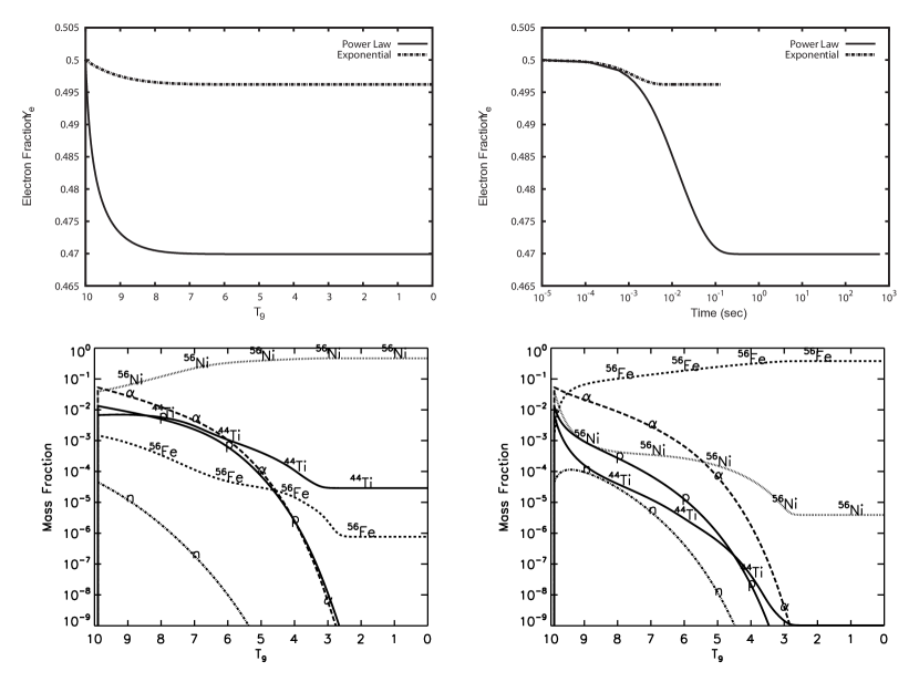
Figure 15: Evolution of the electron fraction $Y_{e}$ versus temperature (upper left) and time (upper right) for the exponential and power-law profiles starting from conditions, $T_{9}=10$ GK, $\rho=10^{10}$ g cm^-3 and $Y_{e}=0.5$, corresponding to the normal freeze-out regime (region 1). The corresponding evolution of the mass fractions are shown for the exponential profile (lower left) and power-law profile (lower right).

In combination with the nucleosynthesis trends for a varying electron fraction (see §5.1 above) and timescale effects, the $\mathrm{p(e^{-},\nu_{e})n}$ and $\mathrm{n(e^{+},\overline{\nu_{e}})p}$ reactions are the key to explaining the chasm’s widening between the exponential and power-law expansions. Depending on the expansion timescale, $\mathrm{p(e^{-},\nu_{e})n}$ and $\mathrm{n(e^{+},\overline{\nu_{e}})p}$ reactions alter the electron fraction only for a limited amount of time early in the evolution. The changes to $Y_{e}$ for various peak temperatures and densities depend on the rate strengths of these reactions and affect the yields directly. Figure 15 shows the evolution of $Y_{e}$ and a few isotopes related to $\mathrm{{}^{44}Ti}$ nucleosynthesis for a case of a normal freeze-out from initially symmetric matter ($Y_{e}=0.5$) using nominal rates for both expansion profiles. In this regime, $\mathrm{p(e^{-},\nu_{e})n}$ always dominates $\mathrm{n(e^{+},\overline{\nu_{e}})p}$ and $Y_{e}$ decreases, while temperature and density still have large values. Timescale effects are evident when using nominal rate values, where the time spent in a high entropy environment is larger for the power-law case and $Y_{e}$ decreases much more compared to the exponential profile. The plasma adjusts to the $Y_{e}\neq 0.5$ conditions while it is still in NSE and QSE subsequently. Figure 13 shows NSE mass fractions as a function of the electron fraction where the production of $\mathrm{{}^{56}Fe}$ is favored, while $\mathrm{{}^{44}Ti}$ and $\mathrm{{}^{56}Ni}$ are under-produced (Hartmann et al., 1985; Woosley & Hoffman, 1992; Seitenzahl et al., 2008). On the contrary, exponential expansion does not allow $Y_{e}$ to decrease significantly, resulting in a final composition with significant yields for $\mathrm{{}^{44}Ti}$ and $\mathrm{{}^{56}Ni}$. Therefore, the chasm expands only for the power-law profile.

The chasm width is regulated primarily by the strength of $\mathrm{p(e^{-},\nu_{e})n}$ and $\mathrm{n(e^{+},\overline{\nu_{e}})p}$ and secondarily by timescale effects. Both ⁴⁴Ti and ⁵⁶Ni show a large chasm expansion for both thermodynamic profiles when these two reactions are enhanced by a factor $10^{3}$. The new chasm widths for the two profiles are similar, because the reaction rate enhancement results in the same decrement to $Y_{e}$ for both thermodynamic profiles and diminishes the impact of timescale effects. In Figure 14, the normal freeze-out regime (region 1) for $\mathrm{{}^{44}Ti}$ merges with the chasm (region 2) and the chasm expands into the area that belonged to the $\alpha$-rich freeze-out regime (region 3).

The remaining weak interactions also assist in the decrement of the electron fraction, and thus to the chasm expansion, but their contributions are smaller than $\mathrm{p(e^{-},\nu_{e})n}$ and $\mathrm{n(e^{+},\overline{\nu_{e}})p}$ due to their lifetimes. The lifetime of any weak interactions that are primarily responsible for the changes to the electron fraction must be smaller than the expansion timescale. In Figure 15 the changes to $Y_{e}$ take place between $10^{-3}\lesssim t\lesssim 10^{-1}$ sec. The exponential profile has a timescale of the order of 1 sec, and the changes to $Y_{e}$ are moderate. On the contrary, the timescale for the power-law is larger by two orders of magnitude, resulting in dramatic changes to $Y_{e}$ due to the impact of $\mathrm{p(e^{-},\nu_{e})n}$, $\mathrm{n(e^{+},\overline{\nu_{e}})p}$, and weak interactions. Despite the initial identical configuration of the two expansions, the equilibrium state that the normal freeze-out begins is very different for the two expansion profiles. For the exponential trajectory, the weak interactions do not have the time to change the equilibrium state adequately, and the final yields have a significant amount of $\mathrm{{}^{44}Ti}$, with $\mathrm{{}^{56}Ni}$ dominating the final composition. For the power-law profile $\mathrm{{}^{56}Fe}$ is the dominant element and $\mathrm{{}^{44}Ti}$ is under-produced, expanding the chasm region into the normal freeze-out regime (see Figure 15). In addition to $\mathrm{p(e^{-},\nu_{e})n}$ and $\mathrm{n(e^{+},\overline{\nu_{e}})p}$ reactions, Table 3 lists the primary weak interactions related to the chasm widening, all with a half life of the order of $10^{-1}$ sec.

Weak interactions assist in defining the $\mathrm{{}^{44}Ti}$ topology for the $\alpha$$p$-rich freeze-out regime (region 4). In this region, $\mathrm{n(e^{+},\overline{\nu_{e}})p}$ dominates over $\mathrm{p(e^{-},\nu_{e})n}$ and $Y_{e}$ rises above 0.5, driving the material proton-rich. The relative strength of the $\mathrm{p(e^{-},\nu_{e})n}$ and $\mathrm{n(e^{+},\overline{\nu_{e}})p}$ rates determines the area of the peak temperature-density plane occupied by the $\alpha$$p$-rich freeze-out regime as shown by Figure 14. Both $\mathrm{{}^{44}Ti}$ and $\mathrm{{}^{56}Ni}$ have significant mass fraction values during equilibrium states in such environments, despite the relatively large mass fractions of proton-rich isotopes. These isotopes decay within the expansion timescale and transfer additional nuclear flow to the symmetric isotopes. Weak reactions partially regulate the second arc for the $\mathrm{{}^{44}Ti}$ mass fraction, and the formation of the ascending track at the end of the freeze-out process.

For $Y_{e}=0.48$ the weak interactions barely have an impact on the $\mathrm{{}^{44}Ti}$ yield. Within the $\alpha$$p$-rich freeze-out regime their action is similar to the symmetric case, but the area that region 4 occupies on the temperature-density plane for neutron-rich matter is limited. Within the $\alpha$-rich freeze-out regime the major flows are localized mostly among stable nuclei, or nuclei with decay timescales much longer than the expansion timescale.

For $Y_{e}=0.52$ the action of the weak interactions has been outlined before. They transfer nuclear flow from proton-rich to symmetric nuclei for most of the peak conditions within the temperature-density plane. For the $\alpha$$p$-rich freeze-out region with the exponential profile, the average half-life range for the primary flow carriers is $90\lesssim t_{1/2}\lesssim 500$ ms. For the power-law expansion, the corresponding range is $200\lesssim t_{1/2}\lesssim 900$ ms. Weak reactions for the $\mathrm{(p,\gamma)}$ leakage regime (region 1 for $Y_{e}=0.52$) are classified according to the way they impact. The first group includes reactions which hinder the flow transfer by $\mathrm{(p,\gamma)}$ reactions when their rates are enhanced. The second group includes reactions which boost the flow transfer by $\mathrm{(p,\gamma)}$ reactions when their rates are diminished. The third group includes reactions which combine the action from the two previous groups. Reactions within the third group make an impact only for the power-law expansion profile. In addition, weak reactions with relatively long half-lives contribute to the amplitude regulation of the third arc in the $\mathrm{{}^{44}Ti}$ mass fraction for the $\alpha$$p$-rich freeze-out regime (see Table 3).

7 Network size effects

Trends in the $\mathrm{{}^{44}Ti}$ yields are controlled by a limited number of reactions. This raises a query about the minimum number of nuclei that are necessary to include in a network calculation such that all relevant physical phenomena are captured. Our reference reaction network contains 489 isotopes, spanning the light nuclei, silicon group, and iron group. To assess network size effects, we compared the $\mathrm{{}^{44}Ti}$ yields in the peak temperature-density plane from the 489 isotope network with the final yields generated by reaction networks with 204, 1341, and 3304 isotopes. Table 1 lists the isotopes used in each network. In addition to the new elements introduced, the larger networks expand into larger both neutron-rich and proton-rich regimes. The addition of new elements beyond the Fe-group has a minimal effect on equilibrium clusters, since for the thermodynamic trajectories of interest the largest partial flows are localized around the Si-group and Fe-group.

For $Y_{e}=0.48$, the final mass fractions are essentially independent of the network size since the major flows occur along the valley of stability, which is modeled adequately by all networks. For $Y_{e}\geqslant 0.5$, the final mass fractions depend on the network size as weak interactions have a larger role. In particular, the 204 isotope network does not include most of the required proton-rich isotopes to accurately describe the nucleosynthesis. The differences compared to our reference network are localized to the $\alpha$$p$-rich freeze-out region for $Y_{e}=0.5$, but they span all the parameter space for $Y_{e}=0.52$. Consequently, this 204 isotope network is inadequate to describe the nucleosynthesis of proton-rich material.

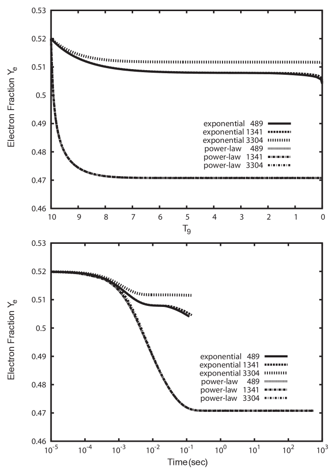
Figure 16: Evolution of the electron fraction $Y_{e}$ for the exponential and power-law freeze-out profiles for a freeze-out starting from $T_{9}=10$ GK, $\rho=10^{10}$ g cm^-3 and $Y_{e}=0.52$, corresponding to the (p,$\gamma$) leakage regime (region 1). The evolution is shown versus temperature (upper plot) and time (lower plot).

There are mass fraction differences in region 1 for $Y_{e}\geqslant 0.5$ between our reference network and the larger networks, which is related to the differences in the equilibrium state configurations by the changes in temperature, density and $Y_{e}$ during the freeze-out evolution. Specifically, the differences are due to the relationship between the expansion and weak interaction timescales. Figure 16 shows the temperature dependence of the electron fraction during a freeze-out for the 489, 1341, and 3304 isotope networks for the exponential and power-law trajectories. The 489 and 1341 isotope networks have relatively similar numbers of isotopes per element, for those elements that are common to both networks. Consequently, the evolution of $Y_{e}$ is quite similar for both profiles. The 3304 isotope network, however, has a larger number of isotopes per element for elements that are common among the three networks (see Table 1). The presence of more proton-rich nuclei in the 3304 isotope network slows the electron fraction decrease driven by $\mathrm{p(e^{-},\nu_{e})n}$ and $\mathrm{n(e^{+},\overline{\nu_{e}})p}$ compared to our reference network. This results in slightly different large scale equilibrium states. For a short expansion timescale, such as the exponential profile, $Y_{e}$ values remain above 0.5 for all networks, resulting in the differences in region 1. The long timescale of the power-law expansion decreases the electron fraction value below 0.5 quite early in the evolution. This results in all three networks converging to the same $Y_{e}$ values since all three networks include the necessary isotopes related to production of $\mathrm{{}^{44}Ti}$ and $\mathrm{{}^{56}Ni}$. Overall, our reference 489 isotope network is adequate for describing the trends in the $\mathrm{{}^{44}Ti}$ and $\mathrm{{}^{56}Ni}$ yield trends. This is relevant for efficient use of computational resources.

8 Post-Process Yields from Collapse Simulations

In this section we compare the ⁴⁴Ti and ⁵⁶Ni yields from post-processing core-collapse supernovae models with the exponential and power-law trajectories. We use the same reference 489 isotope reaction network for the post-processing and parameterized trajectories. Our aim is to offer a calibration of where parameterized trajectories provide a reasonable approximation to the final yields. Our analysis in the preceding sections allows an explanation for the behavior of the ⁴⁴Ti and ⁵⁶Ni profiles and any differences between the post-processed and parameterized yields. For this assessment we consider 3 of the supernova explosion calculations whose tracks in the peak temperature-density plane are shown in Figure 3. In all three of these models the initial $Y_{e}$ profile as a function of interior mass is very close to Ye = 0.5.

8.1 A Cassioppeia A model

Our first supernova model uses a progenitor designed to match the supernova remnant Cassioppeia A (Young et al., 2006; Eriksen et al., 2009), specifically model M16E1.1BinA from Young et al. (2008). The hydrogen envelope of this spherically symmetric 16 M_⊙ progenitor was removed by an assumed binary mass transfer event as the progenitor evolved into a giant. We use a multi-step collapse and explosion process to model the explosion (for example, see Young & Fryer, 2007). We model the entire star from collapse through the formation and stall of the bounce shock. At this point, the proto-neutron star is removed from the simulation and energy is injected just above the proto-neutron star to drive an explosion. The explosion is followed as the shock moves out of the star and most of the fallback has accreted onto the newly-formed neutron star. We only calculate the yields of material that is ejected after fallback.

Mass fraction profiles from post-processing the Lagrangian thermodynamic trajectories with our reference 489 isotope network are shown in the top panel of Figure 17. The iron-group, silicon-group, oxygen-rich shells are visible within the innermost 1.5 M_⊙. The bottom panel shows the mass fraction profiles from the post-process, exponential, and power-law trajectories. Mass fraction profiles correspond to the left-hand y-axis, and the peak temperature and peak density curves correspond to the right-hand y-axis. Figure 3 also shows the peak temperatures and densities of this explosion model, and explains the general trends in the ⁴⁴Ti, ⁵⁶Ni and ⁴He mass fraction profiles of Figure 17.

For interior masses less than $\approx$ 0.2 M_⊙, the synthesis of ⁴⁴Ti is due to the $\alpha$-rich freeze-out, region 3 in Figure 4. In this mass range, the ⁴⁴Ti mass fractions from the power-law profile are closer to the post-process values than the exponential profile. The ⁵⁶Ni mass fractions given by the power-law and exponential profiles generally agree with the post-process mass fractions. Near 0.2 M_⊙, the thin chasm region separating region 3 ($\alpha$-rich freeze-out) and region 6 (silicon-rich) is traversed, which causes the downward spike in the ⁴⁴Ti profile (see Figures 3 and 4). Precisely where the thin chasm is traversed depends sensitively on the exact values of peak temperatures and densities, and the location of the thin chasm line on the temperature-density plane due to the timescale of the expansion profile. This explains why the downward spike occurs at slightly different mass locations for the post-process, exponential and power-law profiles. Between $\approx$ 0.2 M_⊙ and $\approx$ 0.5 M_⊙ the explosion is operating in the silicon-rich, region 6 of Figure 3. In this region the final yields of both ⁴⁴Ti and ⁵⁶Ni are sensitive to the initial composition, which in this case is given by the model at the time when energy is injected just above the proto-neutron star to drive an explosion. In this mass range, the ⁴⁴Ti mass fractions post-processing, exponential, and power-law profiles generally agree. For ⁵⁶Ni, the power-law profile generally agrees with the post-process mass fractions better than the exponential profile. Both ⁴⁴Ti and ⁵⁶Ni abruptly decline at $\approx$ 0.5 M_⊙ as the peak temperature drops below 4$\times$10⁹ K.

Yields from the exponential and power-law trajectories are generally within a factor $\sim$ 2 of the post-process yields, except in region where the thin chasm is being crossed or the temperature falls below 4$\times$10⁹ K. Integrating the ⁴⁴Ti mass fraction profiles in Figure 17 over the interior mass gives the total mass of ⁴⁴Ti ejected by this model. We find 1.04$\times$10^-4 M_⊙ for post-processing, 5.62$\times$10^-5 M_⊙ for the exponential profile, and 9.30$\times$10^-5 M_⊙ for the power-law profile. Similarly for ⁵⁶Ni, we find 2.46$\times$10^-1 M_⊙ for post-processing, 3.16$\times$10^-1 M_⊙ for the exponential profile, and 2.78$\times$10^-1 M_⊙ for the power-law profile. Overall, yields of ⁴⁴Ti and ⁵⁶Ni from the power-law profile mimic the post-process values better than the exponential profile for this Cas A model.

8.2 A Weak-Strong Hypernova Model

Our second massive star explosion model uses a similar multi-step process. In this case however, first a weak explosion is launched and followed 1 s later by a strong $1.6\times 10^{52}{\rm erg}$ hypernova explosion. This model has a very different thermodynamic evolution as the material is hit by two shocks. The first, weaker shock ignites a substantial amount of burning within the inner 0.6 M_⊙. Most of the peak temperatures and peak densities inside 0.6 M_⊙ are due to the weaker shock. Peak conditions at larger masses are due to the second, stronger shock. For additional details on this weak-strong double shock model, see 40WS1.0 from Fryer et al. (2006).

Mass fraction profiles from post-processing the Lagrangian thermodynamic trajectories with our reference 489 isotope network are shown in the top panel of Figure 18. The iron-group and silicon-group shells are visible within the innermost 1.5 M_⊙. The bottom panel of Figure 18 shows the mass fraction profiles from the post-process, exponential, and power-law trajectories. Mass fraction profiles correspond to the left-hand y-axis, and the peak temperature and peak density curves correspond to the right-hand y-axis. Figure 3 also shows the peak temperatures and densities of this explosion model, and explains the general trends in the ⁴⁴Ti and ⁵⁶Ni mass fraction profiles of Figure 18. For interior masses less than $\approx$ 0.4 M_⊙, the synthesis of ⁴⁴Ti is due to the $\alpha$-rich and $\alpha$p-rich freeze-outs, regions 3 and 4 respectively in Figure 4. In this mass range, the ⁴⁴Ti and ⁵⁶Ni mass fractions given by the exponential and power-law profiles have about the same level of agreement with the post-process values. Near 0.4 M_⊙, the thin chasm region separating region 3 ($\alpha$-rich freeze-out) and region 6 (silicon-rich) is traversed, which causes the downward spike in the ⁴⁴Ti profile (see Figures 3 and 4). The downward spike occurs at different mass locations for the post-process, exponential and power-law profiles because when the thin chasm is traversed depends on the exact values of peak temperatures and densities, and the location of the thin chasm line on the temperature-density plane due to the timescale of the expansion profile.

Between $\approx$ 0.4 M_⊙ and $\approx$ 0.7 M_⊙ the explosion is operating in the silicon-rich, region 6 of Figure 3. In this region the final yields of ⁴⁴Ti and ⁵⁶Ni are sensitive to the initial composition. Beyond $\approx$ 0.7 M_⊙ there are two reasons for the rapid decline of the ⁴⁴Ti and ⁵⁶Ni mass fraction profiles from the parameterized trajectories while the post-process mass fraction profiles remain essentially flat at $\approx$ 10^-6 out to 1.5 M_⊙ First, the parameterized trajectories assume an initial composition that is generally pure ²⁸Si (with perhaps some neutrons or protons to adjust $Y_{e}$; see Section 3) which is different than the initial composition of the hypernova model. In region 6 and where peak temperature drops below 4$\times$10⁹ K the yields from the parameterized trajectories are initial composition dependent. Second, the strong shock that follows the weak shock raises the temperature to $\approx$ 3.5$\times$10⁹ K at densities of $\approx$ 10⁶ g cm^-3 out to $\approx$ 1.5 M_⊙. Over another 5 s of evolution, this is sufficient to turn some of the ²⁸Si into ⁴⁴Ti.

Yields from the exponential and power-law trajectories are generally only within an order of magnitude of the post-process yields. Integrating the ⁴⁴Ti mass fraction profiles in Figure 18 over the interior mass gives the total mass of ⁴⁴Ti ejected by this model. We find 2.66$\times$10^-5 M_⊙ for post-processing, 5.23$\times$10^-5 M_⊙ for the exponential profile, and 6.34$\times$10^-5 M_⊙ for the power-law profile. Similarly for ⁵⁶Ni, we find 3.77$\times$10^-1 M_⊙ for post-processing, 4.83$\times$10^-1 M_⊙ for the exponential profile, and 4.97$\times$10^-1 M_⊙ for the power-law profile. When the hydrodynamic evolution is complicated, the post-process and parameterized profile yields will generally not agree, but parameterized profiles still provide guidance on interpreting the post-processed yields.

8.3 A 2D Rotating Supernova Model

Our third model is a 2D explosion of a rotating 15 M_⊙ star (model 1 from Fryer & Heger, 2000). This simulation follows the collapse, bounce, explosion, and includes the entire proto-neutron star throughout the evolution. The dynamical trajectory of the particles, and the time material spends at any location, can play a major role in the final ⁴⁴Ti and ⁵⁶Ni yields. In some cases, the convective motion makes the matter undergo a series of heating-cooling cycles. However, for most matter, these cycles occur well above NSE temperatures and, fortunately, the evolution in the NSE regime does not affect the final yields significantly except through changes in the electron fraction. This rotating supernova model ends at 1.4 s after bounce which has two implications. First, some of the nominal ejecta may still fall back onto the proto-neutron star. That is, some of the particles we post-process may not ultimately be part of the nucleosynthetic yield. Second, most of the particles have temperatures large enough to interfere with a comparison of material that has undergone a complete freeze-out via the exponential or power-law trajectory. To facilitate this comparison we have appended exponential and power-law thermodynamic trajectories to the final time point of the dynamical model. In this manner we extend the thermodynamic evolution to 4.2 s, by which time all the particles have temperatures below 5$\times$10⁸ K. The quantitative differences between the exponential tail and power-law tail appear small enough that we will only show results for the power-law tail.

The top row of Figure 19 shows the peak temperatures and peak densities within the innermost $\sim$ 1.2 M_⊙ at the coordinates reached by all particles at 4.2 s. The equatorial plane is located at y=0, two lobes appear at roughly $\pm$ 45^∘, and the overall geometry is not symmetric due to rotation and convective fluid motions. Most of the peak thermodynamic conditions are within the bounds of our analysis. We ignore those particles with peak temperatures above 1$\times$10¹⁰ K or peak densities above 1$\times$10¹⁰ g cm^-3. The post-process yields of ⁴⁴Ti and ⁵⁶Ni within the innermost $\sim$ 1.2 M_⊙ are shown in the bottom row of Figure 19. Most of the ⁴⁴Ti is created within roughly $\pm$ 15^∘ of the equatorial plane, but split into two distinct regions because of the ⁴⁴Ti chasm, the QSE-leakage region 2 of Figure 4.

The first row of Figure 20 shows the peak temperatures and peak densities as a function of interior mass. There is considerable scatter at almost any mass location due to the asymmetries inherent in the 2D model. Mass fraction profiles of ⁴⁴Ti for the post-process, exponential, and power-law trajectories are compared in the second row of the figure. Between $\approx$ 0.1 M_⊙ and $\approx$ 0.3 M_⊙ the ⁴⁴Ti mass fractions from all three thermodynamic trajectories rapidly decrease because a subset of the particles have peak temperatures and peak densities characteristic of the chasm, the QSE-leakage region 2 of Figure 4. The width of the chasm associated with an exponential profile is narrower than the chasm of a power-law profile, accounting for the power-law ⁴⁴Ti mass fraction profile decreasing more rapidly than the exponential ⁴⁴Ti mass fraction profile in this mass range. As expected from our previous analysis, ⁵⁶Ni undergoes no such phase transition, with the result that all thermodynamic trajectories give values of order unity in this mass range. Between $\approx$ 0.6 M_⊙ and $\approx$ 0.7 M_⊙ a large subset of the particles in the equatorial regions have peak temperatures that drop below 4$\times$10⁹ K (see Figure 20) and traverse the thin chasm. This results in the strong trend towards decreasing ⁴⁴Ti and ⁵⁶Ni mass fraction profiles in this mass range. Beyond $\approx$ 0.6 M_⊙ the two asymmetric lobes of Figure 19 are visible as the two horizonal bands in the second row of Figure 20. The “rain” of points in this mass range is due to the large scatter in the peak thermodynamic conditions, where a number of particles have peak temperatures that drop below 4$\times$10⁹ K and traverse the thin chasm.

Integrating the ⁴⁴Ti mass fraction profiles over the interior mass gives the total mass of ⁴⁴Ti ejected by this model. We find 6.98$\times$10^-5 M_⊙ for post-processing, 5.09$\times$10^-5 M_⊙ for the exponential profile, and 4.82$\times$10^-5 M_⊙ for the power-law profile. Similarly for ⁵⁶Ni, we find 3.89$\times$10^-1 M_⊙ for post-processing, 3.99$\times$10^-1 M_⊙ for the exponential profile, and 4.10$\times$10^-1 M_⊙ for the power-law profile.

Overall, the mass fraction profiles from exponential and power-law trajectories are generally within a factor $\sim$ 4 of the post-process values, except in regions where the chasm is traversed, and the total yields of ⁴⁴Ti and ⁵⁶Ni from the parameterized profiles mimic the post-process yields for this 2D, rotating supernova model.

9 Discussion

We have explored the trends in, and sensitivity to, the $\mathrm{{}^{44}Ti}$ and $\mathrm{{}^{56}Ni}$ yields in the ejecta of three contrasting core-collapse supernovae models. We used yields from two parameterized expansion profiles and compared them to the yields from post-processing trajectories from the core-collapse models.

Both parameterized profiles, the classic exponential and our new power-law expressions, assume a constant $T^{3}/\rho$ adiabat throughout the evolution. For any given peak temperature and peak density initial conditions, the power-law is slower compared to the exponential and together they generally bound the trajectories from core-collapse simulations. We find that $\mathrm{{}^{44}Ti}$ may be produced by more than one type of freeze-out, depending on the peak temperatures, densities and electron fraction values of the thermodynamic trajectories. We have identified several distinct regions in the peak temperature-density plane from the parameterized profiles. Each region is characterized by different types of transitions that the QSE cluster sustains during the evolution. Reactions that break equilibrium are responsible for the flow transfer to the remaining small scale clusters, maintaining their structure until freeze-out. The result is unique mass fraction profiles per region. The transitions are entropy driven, not expansion timescale driven, where the temperature sets an approximate threshold for a transition, while the density at the threshold temperature determines whether the transition takes place or not. The expansion timescale affects the locus of the borders among different regions in the peak temperature-density plane.

For initially symmetric matter, region 1 is the normal freeze-out regime, where no phase transition takes place and the yields from the parameterized profiles are in good agreement with NSE or QSE estimates. Region 2 is the ⁴⁴Ti chasm, where $\mathrm{{}^{44}Ti}$ is depleted as a result of the large scale QSE cluster dissolution to two smaller ones, and the subsequent flow leakage from the Si-group towards the Fe-group nuclei. Region 3 is the $\alpha$-rich freeze-out regime, where the large scale QSE cluster shrinks and shifts upward in mass due to the domination of the 3$\alpha$ forward rate over its inverse. Region 4 is the $\alpha$$p$-rich freeze-out regime, where $\mathrm{p(e^{-},\nu_{e})n}$ and $\mathrm{n(e^{+},\overline{\nu_{e}})p}$ drive the material slightly proton-rich early in the evolution. Region 5 is the regime where photodisintegrations dominate capture reactions. Region 6 is the incomplete Si-burning regime, where the timescales for the plasma to reach large scale QSE or NSE are comparable to the freeze-out timescale, preventing in general their establishment.

Compared to the symmetric case, $\mathrm{{}^{44}Ti}$ and $\mathrm{{}^{56}Ni}$ are gradually underproduced for initial $Y_{e}<0.5$ and become less sensitive to reaction rates. The basic structure of the temperature-density plane is maintained, with the exception that the $\alpha$$p$-rich freeze-out region decreases in size until complete extinction for $Y_{e}\approx 0.46$ due to the absence of free protons in neutron-rich environments, and the $\mathrm{{}^{44}Ti}$ chasm region expands as a result of the $\mathrm{{}^{44}Ti}$ underproduction in the neighboring regions in the temperature-density plane. In addition, the region of $\alpha$$n$-rich freeze-out appears, where both $\mathrm{{}^{44}Ti}$ and $\mathrm{{}^{56}Ni}$ are depleted since they are symmetric isotopes.

For initial $Y_{e}>0.5$ $\mathrm{{}^{44}Ti}$ and $\mathrm{{}^{56}Ni}$ are favored by large scale NSE and QSE equilibria due to the minimization of the Helmholtz energy. This results in $\mathrm{{}^{56}Ni}$ still being one of the dominant yields, although symmetric isotopes are not favored by the major flows once the large scale QSE cluster dissolves. In this electron fraction regime, weak interactions are crucial to $\mathrm{{}^{44}Ti}$ production. The dominance of $\mathrm{n(e^{+},\overline{\nu_{e}})p}$ over $\mathrm{p(e^{-},\nu_{e})n}$ early in the evolution and the rest of the weak interactions later on, results in significant production of symmetric isotopes. Regions 3 and 4 merge to become a regime of $\alpha$$p$-rich freeze-out due to the large proton excess, and the ⁴⁴Ti chasm expands. Region 1 is no longer a normal freeze-out regime, but it is characterized by a phase transition due to the interplay between $\mathrm{(p,\gamma)}$ and weak reactions.

The three core-collapse models we post-processed were a 1D Cassioppeia A model, a 1D double-shock hypernova model, and a 2D rotating 15 M_⊙ model. Mass fractions of $\mathrm{{}^{44}Ti}$ and $\mathrm{{}^{56}Ni}$ from the exponential and power-law trajectories were shown to generally lie within a factor $\sim$ 8 or less of the post-process yields, except in regions where the thin chasm is being crossed or the temperature fell below 4$\times$10⁹ K. The total ejected masses of $\mathrm{{}^{44}Ti}$ and $\mathrm{{}^{56}Ni}$ were shown to be within a factor of $\sim$ 2 or less for all three models. When the thermodynamic trajectories of a core-collapse model have an expansion profile similar to a parameterized expansion of any form, it is generally safe to trust the yields from the parameterized profiles. For more complicated thermodynamic trajectories, the yields from the parameterized profiles should not be trusted, although the parameterized profiles may provide useful information about the underlying physics.

The location of the $\mathrm{{}^{44}Ti}$ chasm region is profile dependent, and its width is minimized for initially symmetric matter but expand dramatically for $Y_{e}\neq$0.5. These trends could account in part for the observed paucity of supernova detected in the light of radioactive $\mathrm{{}^{44}Ti}$. A mass cut in supernovae models where the electron fraction begins to fall below 0.5 may not be the most suitable choice, since the layers above the mass cut are biased to initially symmetric compositions and can produce ample $\mathrm{{}^{44}Ti}$. We find that variations in the $\mathrm{{}^{44}Ti}$/$\mathrm{{}^{56}Ni}$ ratio originate from variations in $\mathrm{{}^{44}Ti}$, since $\mathrm{{}^{56}Ni}$ is produced in large quantities over most of the peak temperature-density plane (Figure 11). Although the massive production of ⁵⁶Ni and its decay to ⁵⁶Co and ⁵⁶Fe outshine every other decay during their lifetime, the decay of ⁴⁴Ti to ⁴⁴Sc and ⁴⁴Ca has a longer lifetime. This implies that measurements of the yield from ⁴⁴Ti may be used to estimate the yield of ⁵⁶Ni (e.g. measure ⁴⁴Ti in Cas A and deduce Cas A’s ⁵⁶Ni yield), assuming the supernova models’ thermodynamic trajectories approximate one of the parameterized profiles and ⁴⁴Ti originates from regions where ⁵⁶Ni was dominant.

Woosley et al. (1973) first defined the notions of the normal and $\alpha$-rich freeze-outs. Using an exponential profile they describe how the various types of freeze-out are driven by the effect of the 3$\alpha$ reaction. They identify 3 regions in the peak temperature-density plane – normal and $\alpha$-rich freeze-outs and the incomplete silicon burning regime – based on the availability of $\alpha$-particles. These 3 regions are bordered with thin lines based on semi-analytical relationships for the timescale required to reach QSE. Their description is constrained to the interplay between the 3$\alpha$ reaction and the large-scale QSE cluster.

Woosley & Hoffman (1992) explored cases of freeze-outs starting at large neutron excesses, resulting in the production of isotopes heavier than the Fe-group and illustrating the smooth merging of the freeze-out process into the r-process. They used the exponential profile for a peak temperature $T_{9}=10$, three different values for the peak density and a grid of initial neutron excesses within the range $0\leqslant\eta\leqslant 0.21$ (corresponding to a range for the electron fraction $0.395\leqslant Y_{e}\leqslant 0.5$). For the specific case of initial $Y_{e}=0.48$ they mentioned that yields for the Fe-group nuclei were not very different from the symmetric case, but the production of heavier nuclei is also possible. This is in agreement with our results (Table 2), where the yields for $\mathrm{{}^{44}Ti}$ and $\mathrm{{}^{56}Ni}$ are decreased but are not negligible compared to the symmetric case, and a region of $\alpha$$n$-rich freeze-out appears in the peak temperature-density planes. Their argument for flows being inhibited beyond $\mathrm{{}^{56}Ni}$ for nearly symmetric compositions is functionally the same as ours. Their argument is based on $Q$ values and other nuclear structure effects around the doubly magic nucleus $\mathrm{{}^{56}Ni}$, which is equivalent to a persistent small equilibrium cluster localized around $\mathrm{{}^{56}Ni}$ until complete freeze-out. Finally, they suggested the possibility of freeze-out expansions with negative neutron excesses ($Y_{e}>0.5$) due to the interplay between $\mathrm{p(e^{-},\nu_{e})n}$ and $\mathrm{n(e^{+},\overline{\nu_{e}})p}$, which we have discussed in detail within this study.

The et al. (1998) conducted the first detailed sensitivity study of reaction rates on the $\mathrm{{}^{44}Ti}$ mass fraction by using the exponential profile and one pair of peak conditions ($T_{9}=5.5$, $\rho=10^{7}$ g cm^-3). They identified a significant amount of reactions affecting $\mathrm{{}^{44}Ti}$, and suggested the impact of $\mathrm{\mathrm{{}^{45}V}(p,\gamma)\mathrm{{}^{46}Cr}}$ and $\mathrm{\mathrm{{}^{12}C}(\alpha,\gamma)\mathrm{{}^{16}O}}$ for $Y_{e}<0.5$. However, the choice of only one set pair of peak conditions and one expansion profile doesn’t allow all crucial reactions identified in all regions.

Recent sensitivity studies have varied rates within their experimental uncertainty limits. Hoffman et al. (2010) used one-zone calculations with results for $\mathrm{{}^{44}Ti}$, $\mathrm{{}^{57}Ni}$, $\mathrm{{}^{58}Ni}$ and $\mathrm{{}^{56}Ni}$ presented in proportion to solar $\mathrm{{}^{56}Fe}$, considering in addition yields for these isotopes from published supernovae models. They varied all published rate compilations of $\mathrm{\mathrm{{}^{44}Ti}(\alpha,p)\mathrm{{}^{47}V}}$ and $\mathrm{\mathrm{{}^{40}Ca}(\alpha,\gamma)\mathrm{{}^{44}Ti}}$ for peak conditions taken from various points within the temperature-density plane given in Magkotsios et al. (2008). They also varied the expansion timescale of the exponential profile, concluding that the yield of $\mathrm{{}^{44}Ti}$ is affected by the time it remains within successive burning stages. Tur et al. (2010) have utilized stellar evolution models to address the impact of the $3\alpha$ and $\mathrm{\mathrm{{}^{12}C}(\alpha,\gamma)\mathrm{{}^{16}O}}$ reactions on $\mathrm{{}^{26}Al}$, $\mathrm{{}^{44}Ti}$ and $\mathrm{{}^{60}Fe}$. They conclude that $\mathrm{{}^{44}Ti}$ is relatively insensitive to these rates, although they comment that this result depends on the explosion physics and supernovae rate assumed. Variations to the $3\alpha$ rate within our study also result in relatively insensitive yields, because only a limited flow is required by this reaction to impact the QSE cluster. In order to illustrate the reaction’s role, it is necessary to remove it completely from network calculations. $\mathrm{\mathrm{{}^{12}C}(\alpha,\gamma)\mathrm{{}^{16}O}}$ has an impact on $\mathrm{{}^{44}Ti}$ mostly for neutron-rich compositions (Table 3).

Our study adds to these works by considering all the freeze-out regions in the peak temperature-density plane over a broad range of $Y_{e}$. The various types of freeze-out may be understood as differing equilibrium patterns during the evolution, where a change to the pattern is usually signaled by individual reactions dropping out of equilibrium. The use of two expansion profiles and detailed sensitivity studies for all regions within the peak temperature-density plane reveals the importance of additional reactions crucial to $\mathrm{{}^{44}Ti}$ synthesis beyond the set first identified by The et al. (1998).

Table 1: NUCLEAR NETWORKS

	204		489		1341		3304
Z	$A_{min}$	$A_{max}$	$A_{min}$	$A_{max}$	$A_{min}$	$A_{max}$	$A_{min}$	$A_{max}$
H	2	3	2	3	2	3	2	3
He	3	3	3	3	3	3	3	3
Li	6	7	6	7	6	9	6	9
Be	7	9	7	9	7	12	7	12
B	8	11	8	11	8	14	8	14
C	11	14	11	14	11	17	9	18
N	13	15	12	15	12	20	11	21
O	14	19	14	19	14	21	13	22
F	17	19	17	21	18	22	16	26
Ne	18	23	17	24	18	29	16	31
Na	21	24	19	27	19	32	17	34
Mg	22	27	20	29	20	37	18	37
Al	25	28	22	31	22	40	20	40
Si	27	32	23	34	23	41	22	43
P	29	34	27	38	27	44	24	46
S	31	37	28	42	28	47	26	49
Cl	33	38	31	45	31	50	28	51
Ar	36	41	32	46	32	53	30	54
K	37	42	35	49	34	58	32	56
Ca	40	49	36	49	36	59	34	59
Sc	41	50	40	51	40	64	36	64
Ti	44	51	41	53	41	55	38	67
V	45	52	43	55	43	68	40	72
Cr	48	55	44	58	44	69	42	75
Mn	51	57	46	61	46	74	44	76
Fe	52	61	47	63	48	74	46	78
Co	55	62	50	65	50	78	48	80
Ni	56	65	51	67	51	80	50	83
Cu	57	66	55	69	57	85	52	86
Zn	60	69	57	72	59	86	54	89
Ga	61	70	59	75	59	94	56	92
Ge	64	71	62	78	62	97	58	95
As	$\cdots$	$\cdots$	65	79	68	103	60	100
Se	$\cdots$	$\cdots$	67	83	63	103	63	103
Br	$\cdots$	$\cdots$	68	83	69	106	65	105
Kr	$\cdots$	$\cdots$	69	87	72	109	68	108
Rb	$\cdots$	$\cdots$	73	85	74	113	74	111
Sr	$\cdots$	$\cdots$	74	84	76	118	73	114
Y	$\cdots$	$\cdots$	75	87	78	121	75	119
Zr	$\cdots$	$\cdots$	78	90	80	122	77	122
Nb	$\cdots$	$\cdots$	82	90	81	123	80	124
Mo	$\cdots$	$\cdots$	83	90	82	125	82	125
Tc	$\cdots$	$\cdots$	89	91	87	127	85	126
Ru	$\cdots$	$\cdots$	$\cdots$	$\cdots$	90	130	86	128
Rh	$\cdots$	$\cdots$	$\cdots$	$\cdots$	93	131	89	130
Pd	$\cdots$	$\cdots$	$\cdots$	$\cdots$	94	132	91	132
Ag	$\cdots$	$\cdots$	$\cdots$	$\cdots$	97	133	93	134
Cd	$\cdots$	$\cdots$	$\cdots$	$\cdots$	98	136	95	134
In	$\cdots$	$\cdots$	$\cdots$	$\cdots$	99	149	97	137
Sn	$\cdots$	$\cdots$	$\cdots$	$\cdots$	102	152	99	140
Sb	$\cdots$	$\cdots$	$\cdots$	$\cdots$	$\cdots$	$\cdots$	105	151
Te	$\cdots$	$\cdots$	$\cdots$	$\cdots$	$\cdots$	$\cdots$	109	154
I	$\cdots$	$\cdots$	$\cdots$	$\cdots$	$\cdots$	$\cdots$	112	158
Xe	$\cdots$	$\cdots$	$\cdots$	$\cdots$	$\cdots$	$\cdots$	113	161
Cs	$\cdots$	$\cdots$	$\cdots$	$\cdots$	$\cdots$	$\cdots$	118	165
Ba	$\cdots$	$\cdots$	$\cdots$	$\cdots$	$\cdots$	$\cdots$	119	168
La	$\cdots$	$\cdots$	$\cdots$	$\cdots$	$\cdots$	$\cdots$	122	172
Ce	$\cdots$	$\cdots$	$\cdots$	$\cdots$	$\cdots$	$\cdots$	122	175
Pr	$\cdots$	$\cdots$	$\cdots$	$\cdots$	$\cdots$	$\cdots$	126	178
Nd	$\cdots$	$\cdots$	$\cdots$	$\cdots$	$\cdots$	$\cdots$	127	178
Pm	$\cdots$	$\cdots$	$\cdots$	$\cdots$	$\cdots$	$\cdots$	130	185
Sm	$\cdots$	$\cdots$	$\cdots$	$\cdots$	$\cdots$	$\cdots$	133	188
Eu	$\cdots$	$\cdots$	$\cdots$	$\cdots$	$\cdots$	$\cdots$	136	190
Gd	$\cdots$	$\cdots$	$\cdots$	$\cdots$	$\cdots$	$\cdots$	139	191
Tb	$\cdots$	$\cdots$	$\cdots$	$\cdots$	$\cdots$	$\cdots$	142	192
Dy	$\cdots$	$\cdots$	$\cdots$	$\cdots$	$\cdots$	$\cdots$	143	193
Ho	$\cdots$	$\cdots$	$\cdots$	$\cdots$	$\cdots$	$\cdots$	146	196
Er	$\cdots$	$\cdots$	$\cdots$	$\cdots$	$\cdots$	$\cdots$	148	198
Tm	$\cdots$	$\cdots$	$\cdots$	$\cdots$	$\cdots$	$\cdots$	150	198
Yb	$\cdots$	$\cdots$	$\cdots$	$\cdots$	$\cdots$	$\cdots$	152	200
Lu	$\cdots$	$\cdots$	$\cdots$	$\cdots$	$\cdots$	$\cdots$	156	209
Hf	$\cdots$	$\cdots$	$\cdots$	$\cdots$	$\cdots$	$\cdots$	159	212
Ta	$\cdots$	$\cdots$	$\cdots$	$\cdots$	$\cdots$	$\cdots$	161	217
W	$\cdots$	$\cdots$	$\cdots$	$\cdots$	$\cdots$	$\cdots$	163	220
Re	$\cdots$	$\cdots$	$\cdots$	$\cdots$	$\cdots$	$\cdots$	167	225
Os	$\cdots$	$\cdots$	$\cdots$	$\cdots$	$\cdots$	$\cdots$	169	226
Ir	$\cdots$	$\cdots$	$\cdots$	$\cdots$	$\cdots$	$\cdots$	172	230
Pt	$\cdots$	$\cdots$	$\cdots$	$\cdots$	$\cdots$	$\cdots$	175	232
Au	$\cdots$	$\cdots$	$\cdots$	$\cdots$	$\cdots$	$\cdots$	178	236
Hg	$\cdots$	$\cdots$	$\cdots$	$\cdots$	$\cdots$	$\cdots$	178	239
Tl	$\cdots$	$\cdots$	$\cdots$	$\cdots$	$\cdots$	$\cdots$	182	245
Pb	$\cdots$	$\cdots$	$\cdots$	$\cdots$	$\cdots$	$\cdots$	185	246
Bi	$\cdots$	$\cdots$	$\cdots$	$\cdots$	$\cdots$	$\cdots$	188	251
Po	$\cdots$	$\cdots$	$\cdots$	$\cdots$	$\cdots$	$\cdots$	193	237
At	$\cdots$	$\cdots$	$\cdots$	$\cdots$	$\cdots$	$\cdots$	210	211

Table 2: FREEZE-OUT DOMINANT YIELDS

Freeze-out	$\rho_{peak}$ (g cm-3)	Exponential	Power-Law
$Y_{e}=0.48$, $T_{9}=9$
Normal	$5\times 10^{9}$	$\mathrm{{}^{54}Fe}$, $\mathrm{{}^{58}Ni}$, $\mathrm{{}^{56}Fe}$, $\mathrm{{}^{55}Fe}$, $\mathrm{{}^{60}Ni}$	$\mathrm{{}^{54}Fe}$, $\mathrm{{}^{56}Fe}$, $\mathrm{{}^{58}Ni}$, $\mathrm{{}^{60}Ni}$, $\mathrm{{}^{55}Fe}$
$\alpha$-rich	$10^{7}$	$\mathrm{{}^{58}Ni}$, $\mathrm{{}^{4}He}$, $\mathrm{{}^{60}Ni}$, $\mathrm{{}^{64}Zn}$, $\mathrm{{}^{62}Zn}$	$\mathrm{{}^{58}Ni}$, $\mathrm{{}^{4}He}$, $\mathrm{{}^{60}Ni}$, $\mathrm{{}^{64}Zn}$, $\mathrm{{}^{62}Zn}$
$\alpha$$p$-rich	$\cdots$	$\cdots$	$\cdots$
$\alpha$$n$-rich	$5\times 10^{4}$ ($T_{9}=6$)	$\mathrm{{}^{4}He}$, $\mathrm{{}^{87}Kr}$, n, $\mathrm{{}^{49}Ca}$, $\mathrm{{}^{83}Se}$	$\mathrm{{}^{4}He}$, n, $\mathrm{{}^{49}Ca}$, $\mathrm{{}^{87}Kr}$, $\mathrm{{}^{72}Zn}$
$Y_{e}=0.50$, $T_{9}=9$
Normal	$5\times 10^{9}$	$\mathrm{{}^{56}Ni}$, $\mathrm{{}^{54}Fe}$, $\mathrm{{}^{52}Fe}$, $\mathrm{{}^{55}Co}$, $\mathrm{{}^{57}Ni}$	$\mathrm{{}^{54}Fe}$, $\mathrm{{}^{58}Ni}$, $\mathrm{{}^{56}Ni}$, $\mathrm{{}^{55}Fe}$, $\mathrm{{}^{56}Fe}$
$\alpha$-rich	$10^{8}$	$\mathrm{{}^{56}Ni}$, $\mathrm{{}^{4}He}$, $\mathrm{{}^{60}Zn}$, $\mathrm{{}^{57}Ni}$, $\mathrm{{}^{58}Cu}$	$\mathrm{{}^{56}Ni}$, $\mathrm{{}^{60}Cu}$, $\mathrm{{}^{4}He}$, $\mathrm{{}^{57}Ni}$, $\mathrm{{}^{58}Ni}$
$\alpha$$p$-rich	$10^{6}$	$\mathrm{{}^{4}He}$, $\mathrm{{}^{56}Ni}$, p, $\mathrm{{}^{60}Zn}$, $\mathrm{{}^{52}Fe}$	$\mathrm{{}^{4}He}$, $\mathrm{{}^{56}Ni}$, p, $\mathrm{{}^{60}Cu}$, $\mathrm{{}^{52}Fe}$
$\alpha$$n$-rich	$\cdots$	$\cdots$	$\cdots$
$Y_{e}=0.52$, $T_{9}=9$
$\mathrm{(p,\gamma)}$ leakage	$10^{8}$ ($T_{9}=5$)	$\mathrm{{}^{56}Ni}$, $\mathrm{{}^{58}Cu}$, $\mathrm{{}^{59}Cu}$, $\mathrm{{}^{58}Ni}$, $\mathrm{{}^{57}Ni}$	$\mathrm{{}^{56}Ni}$, $\mathrm{{}^{60}Cu}$, $\mathrm{{}^{59}Ni}$, $\mathrm{{}^{60}Zn}$, $\mathrm{{}^{60}Ni}$
$\alpha$-rich	$\cdots$	$\cdots$	$\cdots$
$\alpha$$p$-rich	$10^{7}$	$\mathrm{{}^{56}Ni}$, $\mathrm{{}^{4}He}$, p, $\mathrm{{}^{60}Zn}$, $\mathrm{{}^{57}Ni}$	$\mathrm{{}^{56}Ni}$, $\mathrm{{}^{4}He}$, p, $\mathrm{{}^{57}Ni}$, $\mathrm{{}^{60}Cu}$
$\alpha$$n$-rich	$\cdots$	$\cdots$	$\cdots$

Table 3: NUCLEAR REACTIONS RELEVANT TO $\mathrm{{}^{44}Ti}$ SYNTHESIS

Reaction	Contribution	Rank	$Y_{e}$	Region	Profile
Global scope reactions
3$\alpha$	flow transfer to QSE cluster	primary	0.48-0.52	2-5	both
$\mathrm{p(e^{-},\nu_{e})n}$ / $\mathrm{n(e^{+},\overline{\nu_{e}})p}$	$Y_{e}$ adjustment	primary	0.48-0.52	1-5	both
$\mathrm{p(e^{-},\nu_{e})n}$ / $\mathrm{n(e^{+},\overline{\nu_{e}})p}$	chasm widening	primary	0.50-0.52	2	both
$\mathrm{(\alpha,\gamma)}$ reactions
$\mathrm{\mathrm{{}^{40}Ca}(\alpha,\gamma)\mathrm{{}^{44}Ti}}$	2nd arc amplitude/slope	primary	0.48-0.52	3-4	both
$\mathrm{\mathrm{{}^{12}C}(\alpha,\gamma)\mathrm{{}^{16}O}}$	flow transfer to QSE cluster	secondary	0.48	2-5	both
$\mathrm{\mathrm{{}^{7}Be}(\alpha,\gamma)\mathrm{{}^{11}C}}$	chasm depth	secondary	0.5	2	both
$\mathrm{\mathrm{{}^{24}Mg}(\alpha,\gamma)\mathrm{{}^{28}Si}}$	chasm depth	secondary	0.5	2	both
$\mathrm{\mathrm{{}^{42}Ca}(\alpha,\gamma)\mathrm{{}^{46}Ti}}$	chasm depth, 1st arc dip	secondary	0.48	2-3	both
$\mathrm{(\alpha,p)}$ reactions
$\mathrm{\mathrm{{}^{44}Ti}(\alpha,p)\mathrm{{}^{47}V}}$	chasm formation, depth, shift	primary	0.48-0.52	2	both
$\mathrm{\mathrm{{}^{44}Ti}(\alpha,p)\mathrm{{}^{47}V}}$	1st arc dip / 2nd arc slope	primary	0.48-0.50	3-4	both
$\mathrm{\mathrm{{}^{44}Ti}(\alpha,p)\mathrm{{}^{47}V}}$	1st arc dip	primary	0.52	1	both
$\mathrm{\mathrm{{}^{40}Ca}(\alpha,p)\mathrm{{}^{43}Sc}}$	2nd arc dip/slope	primary	0.48-0.50	3-4	both
$\mathrm{\mathrm{{}^{17}F}(\alpha,p)\mathrm{{}^{20}Ne}}$	1st arc dip	primary	0.52	1	both
$\mathrm{\mathrm{{}^{21}Na}(\alpha,p)\mathrm{{}^{24}Mg}}$	1st arc dip	primary	0.52	1	both
$\mathrm{\mathrm{{}^{40}Ca}(\alpha,p)\mathrm{{}^{43}Sc}}$	3rd arc amplitude	secondary	0.52	4	power-law
$\mathrm{\mathrm{{}^{27}Al}(\alpha,p)\mathrm{{}^{30}Si}}$	chasm depth	secondary	0.5	2	exponential
$\mathrm{\mathrm{{}^{55}Co}(\alpha,p)\mathrm{{}^{58}Ni}}$	chasm depth	secondary	0.5	2	exponential
$\mathrm{\mathrm{{}^{48}Cr}(\alpha,p)\mathrm{{}^{51}Mn}}$	chasm depth	secondary	0.5	2	exponential
$\mathrm{\mathrm{{}^{17}F}(\alpha,p)\mathrm{{}^{20}Ne}}$	chasm depth	secondary	0.5	2	exponential
$\mathrm{\mathrm{{}^{52}Fe}(\alpha,p)\mathrm{{}^{55}Co}}$	chasm depth	secondary	0.5	2	exponential
$\mathrm{\mathrm{{}^{54}Fe}(\alpha,p)\mathrm{{}^{57}Co}}$	chasm depth	secondary	0.5	2	exponential
$\mathrm{\mathrm{{}^{21}Na}(\alpha,p)\mathrm{{}^{24}Mg}}$	chasm depth	secondary	0.5	2	exponential
$\mathrm{\mathrm{{}^{56}Ni}(\alpha,p)\mathrm{{}^{59}Cu}}$	chasm depth	secondary	0.5	2	exponential
$\mathrm{\mathrm{{}^{6}Li}(\alpha,p)\mathrm{{}^{9}Be}}$	chasm depth	secondary	0.5	2	power-law
$\mathrm{\mathrm{{}^{13}N}(\alpha,p)\mathrm{{}^{16}O}}$	chasm depth	secondary	0.5	2	power-law
$\mathrm{\mathrm{{}^{42}Ca}(\alpha,p)\mathrm{{}^{45}Sc}}$	1st arc dip / 2nd arc slope	secondary	0.48	3	both
$\mathrm{\mathrm{{}^{43}Sc}(\alpha,p)\mathrm{{}^{46}Ti}}$	1st arc dip	secondary	0.48	3	both
$\mathrm{\mathrm{{}^{58}Ni}(\alpha,p)\mathrm{{}^{61}Cu}}$	2nd arc amplitude	secondary	0.48	3	both
$\mathrm{\mathrm{{}^{38}Ca}(\alpha,p)\mathrm{{}^{41}Sc}}$	1st arc dip	secondary	0.52	1	both
$\mathrm{\mathrm{{}^{34}Ar}(\alpha,p)\mathrm{{}^{37}K}}$	3rd arc amplitude	secondary	0.52	4	power-law
$\mathrm{\mathrm{{}^{38}Ca}(\alpha,p)\mathrm{{}^{41}Sc}}$	3rd arc amplitude	secondary	0.52	4	power-law
$\mathrm{(p,\gamma)}$ reactions
$\mathrm{\mathrm{{}^{45}V}(p,\gamma)\mathrm{{}^{46}Cr}}$	2nd arc formation/dip	primary	0.50-0.52	1,3,4	both
$\mathrm{\mathrm{{}^{45}V}(p,\gamma)\mathrm{{}^{46}Cr}}$	3rd arc formation	primary	0.52	4	power-law
$\mathrm{\mathrm{{}^{41}Sc}(p,\gamma)\mathrm{{}^{42}Ti}}$	2nd arc dip	primary	0.5	4	both
$\mathrm{\mathrm{{}^{43}Sc}(p,\gamma)\mathrm{{}^{44}Ti}}$	2nd arc dip	primary	0.5	4	both
$\mathrm{\mathrm{{}^{44}Ti}(p,\gamma)\mathrm{{}^{45}V}}$	2nd arc dip / 3rd arc formation	primary	0.5	4	both
$\mathrm{\mathrm{{}^{44}Ti}(p,\gamma)\mathrm{{}^{45}V}}$	$\mathrm{\mathrm{{}^{44}Ti}-\mathrm{{}^{45}V}}$ cluster	primary	0.5	4	both
$\mathrm{\mathrm{{}^{41}Sc}(p,\gamma)\mathrm{{}^{42}Ti}}$	2nd arc dip	primary	0.5, 0.52	4	both
$\mathrm{\mathrm{{}^{57}Ni}(p,\gamma)\mathrm{{}^{58}Cu}}$	flow transfer within QSE cluster	primary	0.5	3	both
$\mathrm{\mathrm{{}^{45}V}(p,\gamma)\mathrm{{}^{46}Cr}}$	regions 3-4 borderline	secondary	0.5	3-4	both
$\mathrm{\mathrm{{}^{40}Ca}(p,\gamma)\mathrm{{}^{41}Sc}}$	post-2nd dip track	secondary	0.5	4	both
$\mathrm{\mathrm{{}^{44}V}(p,\gamma)\mathrm{{}^{45}Cr}}$	post-2nd dip track	secondary	0.52	1,4	both
$\mathrm{\mathrm{{}^{43}Ti}(p,\gamma)\mathrm{{}^{44}V}}$	post-2nd dip track	secondary	0.52	1,4	both
$\mathrm{\mathrm{{}^{42}Sc}(p,\gamma)\mathrm{{}^{43}Ti}}$	post-2nd dip track	secondary	0.52	1,4	both
$\mathrm{\mathrm{{}^{57}Cu}(p,\gamma)\mathrm{{}^{58}Zn}}$	post-2nd dip track	secondary	0.52	1,4	both
$\mathrm{\mathrm{{}^{20}Ne}(p,\gamma)\mathrm{{}^{21}Na}}$	post-2nd dip track	secondary	0.52	1,4	both
$\mathrm{\mathrm{{}^{47}V}(p,\gamma)\mathrm{{}^{48}Cr}}$	post-2nd dip track	secondary	0.52	1,4	both
$\mathrm{\mathrm{{}^{43}Sc}(p,\gamma)\mathrm{{}^{44}Ti}}$	post-2nd dip track	secondary	0.48, 0.52	1,3,4	both
$\mathrm{\mathrm{{}^{43}Ti}(p,\gamma)\mathrm{{}^{44}V}}$	3rd arc amplitude	secondary	0.52	4	power-law
$\mathrm{\mathrm{{}^{41}Sc}(p,\gamma)\mathrm{{}^{42}Ti}}$	3rd arc amplitude	secondary	0.52	4	power-law
$\mathrm{\mathrm{{}^{43}Sc}(p,\gamma)\mathrm{{}^{44}Ti}}$	3rd arc amplitude	secondary	0.52	4	power-law
$\mathrm{\mathrm{{}^{40}Ca}(p,\gamma)\mathrm{{}^{41}Sc}}$	post-2nd dip track	secondary	0.52	4	exponential
$\mathrm{\mathrm{{}^{40}Ca}(p,\gamma)\mathrm{{}^{41}Sc}}$	3rd arc amplitude	secondary	0.52	4	power-law
$\mathrm{\mathrm{{}^{42}Ca}(p,\gamma)\mathrm{{}^{43}Sc}}$	2nd arc slope	secondary	0.48	3	both
$\mathrm{\mathrm{{}^{39}K}(p,\gamma)\mathrm{{}^{40}Ca}}$	2nd arc slope	secondary	0.48	3	exponential
$\mathrm{\mathrm{{}^{57}Co}(p,\gamma)\mathrm{{}^{58}Ni}}$	chasm depth	secondary	0.5	2	exponential
$\mathrm{\mathrm{{}^{54}Fe}(p,\gamma)\mathrm{{}^{55}Co}}$	chasm depth	secondary	0.5	2	exponential
$\mathrm{\mathrm{{}^{52}Mn}(p,\gamma)\mathrm{{}^{53}Fe}}$	chasm depth	secondary	0.5	2	exponential
$\mathrm{\mathrm{{}^{57}Ni}(p,\gamma)\mathrm{{}^{58}Cu}}$	regions 3-4 borderline	secondary	0.5	3-4	both
weak reactions
$\mathrm{\mathrm{{}^{54}Co}(e^{-},\nu_{e})\mathrm{{}^{54}Fe}}$	chasm widening	primary	0.50-0.52	2	both
$\mathrm{\mathrm{{}^{50}Mn}(e^{-},\nu_{e})\mathrm{{}^{50}Cr}}$	chasm widening	primary	0.50-0.52	2	both
$\mathrm{\mathrm{{}^{55}Ni}(e^{-},\nu_{e})\mathrm{{}^{55}Co}}$	chasm widening	primary	0.50-0.52	2	both
$\mathrm{\mathrm{{}^{57}Cu}(e^{-},\nu_{e})\mathrm{{}^{57}Ni}}$	chasm widening	primary	0.50-0.52	2	both
$\mathrm{\mathrm{{}^{53}Co}(e^{-},\nu_{e})\mathrm{{}^{53}Fe}}$	chasm widening	primary	0.50-0.52	2	both
$\mathrm{\mathrm{{}^{51}Fe}(e^{-},\nu_{e})\mathrm{{}^{51}Mn}}$	chasm widening	primary	0.50-0.52	2	both
$\mathrm{\mathrm{{}^{58}Cu}(e^{-},\nu_{e})\mathrm{{}^{58}Ni}}$	chasm widening	primary	0.50-0.52	2	power-law
$\mathrm{\mathrm{{}^{59}Cu}(e^{-},\nu_{e})\mathrm{{}^{59}Ni}}$	chasm widening	primary	0.50-0.52	2	power-law
$\mathrm{\mathrm{{}^{42}Ti}(e^{-},\nu_{e})\mathrm{{}^{42}Sc}}$	2nd arc dip / post-2nd dip track	primary	0.50-0.52	4	both
$\mathrm{\mathrm{{}^{41}Sc}(e^{-},\nu_{e})\mathrm{{}^{41}Ca}}$	2nd arc dip / post-2nd dip track	primary	0.50-0.52	4	both
$\mathrm{\mathrm{{}^{43}Ti}(e^{-},\nu_{e})\mathrm{{}^{43}Sc}}$	2nd arc dip / post-2nd dip track	primary	0.50-0.52	4	both
$\mathrm{\mathrm{{}^{44}V}(e^{-},\nu_{e})\mathrm{{}^{44}Ti}}$	2nd arc dip / post-2nd dip track	primary	0.50-0.52	4	both
$\mathrm{\mathrm{{}^{44}V}(e^{-},\nu_{e})\mathrm{{}^{44}Ti}}$	2nd arc dip / post-2nd dip track	primary	0.52	4	exponential
$\mathrm{\mathrm{{}^{38}Ca}(e^{-},\nu_{e})\mathrm{{}^{38}K}}$	2nd arc dip / post-2nd dip track	primary	0.52	4	power-law
$\mathrm{\mathrm{{}^{39}Ca}(e^{-},\nu_{e})\mathrm{{}^{39}K}}$	2nd arc dip / post-2nd dip track	primary	0.52	4	power-law
$\mathrm{\mathrm{{}^{30}S}(e^{-},\nu_{e})\mathrm{{}^{30}P}}$	flow transfer to symmetric nuclei	primary	0.52	1	both
$\mathrm{\mathrm{{}^{57}Cu}(e^{-},\nu_{e})\mathrm{{}^{57}Ni}}$	flow transfer to symmetric nuclei	primary	0.52	1	both
$\mathrm{\mathrm{{}^{34}Ar}(e^{-},\nu_{e})\mathrm{{}^{34}Cl}}$	flow transfer to symmetric nuclei	primary	0.52	1	both
$\mathrm{\mathrm{{}^{42}Ti}(e^{-},\nu_{e})\mathrm{{}^{42}Sc}}$	flow transfer to symmetric nuclei	primary	0.52	1	both
$\mathrm{\mathrm{{}^{44}V}(e^{-},\nu_{e})\mathrm{{}^{44}Ti}}$	flow transfer to symmetric nuclei	primary	0.52	1	exponential
$\mathrm{\mathrm{{}^{45}Cr}(e^{-},\nu_{e})\mathrm{{}^{45}V}}$	flow transfer to symmetric nuclei	primary	0.52	1	power-law
$\mathrm{\mathrm{{}^{55}Ni}(e^{-},\nu_{e})\mathrm{{}^{55}Co}}$	flow transfer to symmetric nuclei	secondary	0.52	1	power-law
$\mathrm{\mathrm{{}^{58}Zn}(e^{-},\nu_{e})\mathrm{{}^{58}Cu}}$	flow transfer to symmetric nuclei	secondary	0.52	1	both
$\mathrm{\mathrm{{}^{43}Ti}(e^{-},\nu_{e})\mathrm{{}^{43}Sc}}$	flow transfer to symmetric nuclei	secondary	0.52	1	power-law
$\mathrm{\mathrm{{}^{41}Ti}(e^{-},\nu_{e})\mathrm{{}^{41}Sc}}$	flow transfer to symmetric nuclei	secondary	0.52	1	power-law
$\mathrm{\mathrm{{}^{45}V}(e^{-},\nu_{e})\mathrm{{}^{45}Ti}}$	flow transfer to symmetric nuclei	secondary	0.52	1	power-law
$\mathrm{\mathrm{{}^{37}Ca}(e^{-},\nu_{e})\mathrm{{}^{37}K}}$	flow transfer to symmetric nuclei	secondary	0.52	1	power-law
$\mathrm{\mathrm{{}^{37}Ca}(e^{-},\nu_{e})\mathrm{{}^{37}K}}$	2nd arc dip / post-2nd dip track	secondary	0.52	4	power-law
$\mathrm{\mathrm{{}^{34}Ar}(e^{-},\nu_{e})\mathrm{{}^{34}Cl}}$	2nd arc dip / post-2nd dip track	secondary	0.52	4	power-law
$\mathrm{\mathrm{{}^{57}Cu}(e^{-},\nu_{e})\mathrm{{}^{57}Ni}}$	2nd arc dip / post-2nd dip track	secondary	0.52	4	power-law
$\mathrm{\mathrm{{}^{34}Ar}(e^{-},\nu_{e})\mathrm{{}^{34}Cl}}$	3rd arc amplitude	secondary	0.52	4	power-law
$\mathrm{\mathrm{{}^{38}Ca}(e^{-},\nu_{e})\mathrm{{}^{38}K}}$	3rd arc amplitude	secondary	0.52	4	power-law
$\mathrm{\mathrm{{}^{39}Ca}(e^{-},\nu_{e})\mathrm{{}^{39}K}}$	3rd arc amplitude	secondary	0.52	4	power-law
$\mathrm{\mathrm{{}^{42}Ti}(e^{-},\nu_{e})\mathrm{{}^{42}Sc}}$	3rd arc amplitude	secondary	0.52	4	power-law
$\mathrm{\mathrm{{}^{57}Cu}(e^{-},\nu_{e})\mathrm{{}^{57}Ni}}$	3rd arc amplitude	secondary	0.52	4	power-law
$\mathrm{(p,n)}$ and $\mathrm{(\alpha,n)}$ reactions
$\mathrm{\mathrm{{}^{57}Co}(p,n)\mathrm{{}^{57}Ni}}$	chasm widening	secondary	0.5	2	both
$\mathrm{\mathrm{{}^{56}Co}(p,n)\mathrm{{}^{56}Ni}}$	chasm widening	secondary	0.5	2	both
$\mathrm{\mathrm{{}^{27}Al}(p,n)\mathrm{{}^{27}Si}}$	chasm widening	secondary	0.5	2	both
$\mathrm{\mathrm{{}^{11}B}(p,n)\mathrm{{}^{11}C}}$	chasm widening	secondary	0.5	2	both
$\mathrm{\mathrm{{}^{10}B}(\alpha,n)\mathrm{{}^{13}N}}$	chasm widening	secondary	0.5	2	both
$\mathrm{\mathrm{{}^{11}B}(\alpha,n)\mathrm{{}^{14}N}}$	chasm widening	secondary	0.5	2	both
$\mathrm{\mathrm{{}^{20}Ne}(\alpha,n)\mathrm{{}^{23}Mg}}$	chasm widening	secondary	0.5	2	both
$\mathrm{\mathrm{{}^{9}Be}(\alpha,n)\mathrm{{}^{12}C}}$	chasm widening	secondary	0.5	2	both
$\mathrm{\mathrm{{}^{42}Ca}(\alpha,n)\mathrm{{}^{45}Ti}}$	1st arc dip / 2nd arc slope	secondary	0.48	3	both
$\mathrm{\mathrm{{}^{34}S}(\alpha,n)\mathrm{{}^{37}Ar}}$	2nd arc amplitude	secondary	0.48	3	both

Figure 2: Schematic temperature or density evolution for the exponential (dashed) and power-law (solid) profiles. For either of the two initial values illustrated, the exponential profile declines faster than the power-law profile. Passages through different burning regimes are indicated.

Figure 5: Mass fraction evolution of ²⁸Si, ⁴⁴Ti, ⁵⁶Ni, neutrons, protons, and $\alpha$-particles for the exponential (left column) and power-law (right column) expansions at $Y_{e}$=0.5. In each panel the peak temperature is 9$\times$10⁹ K. The top row corresponds to region 1 in Figure 4 ($\rho=5\times 10^{9}$ g cm^-3), second row to region 2 ($\rho=1.75\times 10^{9}$ g cm^-3), third row to region 3 ($\rho=1\times 10^{8}$ g cm^-3), and fourth row to region 4 ($\rho=1\times 10^{6}$ g cm^-3).

Figure 7: Reaction network (solid curves) and QSE solutions (dashed and dot-dashed curves) for ⁴⁴Ti (upper left), ⁴⁰Ca (lower left), and ⁴⁸Cr (lower right). Each element shows the characteristic arc driven by equilibrium $(\alpha,p)$ and $(p,\gamma)$ reactions. Beginning at the local minima and onwards to lower temperatures only $(p,\gamma)$ reactions remain in equilibrium, which drive the mass fractions to larger values. This general behavior applies to most of the elements within the silicon and iron groups (small sample upper right).

Figure 17: Mass fractions from post-processing the Lagrangian thermodynamic trajectories (top panel) and post-processing vs parameterized profiles (bottom panel) for the 16 M_⊙ Cas A model (Young et al., 2008). See text for a discussion of the sharp dip in ⁴⁴Ti $\approx$ 0.2 M_⊙, and the decline of ⁴⁴Ti and ⁵⁶Ni $\approx$ 0.6 M_⊙.

Figure 18: Mass fractions from post-processing the Lagrangian thermodynamic trajectories (top panel) and post-processing vs parameterized profiles (bottom panel) for the spherically symmetric 40 M_⊙ hypernova model (Fryer et al., 2006) that features a weak shock followed by a strong shock, with our reference 489 isotope network. Note the sharp dip in ⁴⁴Ti $\approx$ 0.4 M_⊙, and the extended ⁴⁴Ti and ⁵⁶Ni distributions for the post-processed trajectories.

Figure 19: Peak temperatures and peak densities (top row) and mass fractions of ⁴⁴Ti and ⁵⁶Ni (bottom row) generated by the innermost regions in a 2D explosion of a rotating 15 M_⊙ star (Fryer & Heger, 2000). Particles coordinates are shown at 1.4 s, the end of the dynamical model. Note the y=0 equatorial plane, the double lobbed structure, the general asymmetry of the model and evidence for the ⁴⁴Ti chasm along the equatorial regions.

Figure 20: Peak temperatures in grey and peak densities in purple (first row), and comparison of post-process vs parameterized ⁴⁴Ti (second row) and ⁵⁶Ni (third row) profiles as a function of interior mass for the 2D explosion of a rotating 15 M_⊙ star. The scatter is due to the asymmetries of the model.

References

- Aprahamian et al. (2005) Aprahamian, A., Langanke, K., & Wiescher, M. 2005, Progress in Particle and Nuclear Physics, 54, 535
- Arnett et al. (2008) Arnett, D., Meakin, C., & Young, P. A. 2008, ApJ
- Arnett (1977) Arnett, W. D. 1977, ApJS, 35, 145
- Arnett et al. (1989) Arnett, W. D., Bahcall, J. N., Kirshner, R. P., & Woosley, S. E. 1989, ARA&A, 27, 629
- Bodansky et al. (1968) Bodansky, D., Clayton, D. D., & Fowler, W. A. 1968, ApJS, 16, 299
- Bruenn et al. (2006) Bruenn, S. W., Dirk, C. J., Mezzacappa, A., Hayes, J. C., Blondin, J. M., Hix, W. R., & Messer, O. E. B. 2006, Journal of Physics Conference Series, 46, 393
- Buras et al. (2006) Buras, R., Janka, H.-T., Rampp, M., & Kifonidis, K. 2006, A&A, 457, 281
- Calder et al. (2007) Calder, A. C., Townsley, D. M., Seitenzahl, I. R., Peng, F., Messer, O. E. B., Vladimirova, N., Brown, E. F., Truran, J. W., & Lamb, D. Q. 2007, ApJ, 656, 313
- Eriksen et al. (2009) Eriksen, K. A., Arnett, D., McCarthy, D. W., & Young, P. 2009, ApJ, 697, 29
- Fowler & Hoyle (1964) Fowler, W. A., & Hoyle, F. 1964, ApJS, 9, 201
- Fröhlich et al. (2006) Fröhlich, C., Hauser, P., Liebendörfer, M., Martínez-Pinedo, G., Thielemann, F.-K., Bravo, E., Zinner, N. T., Hix, W. R., Langanke, K., Mezzacappa, A., & Nomoto, K. 2006, ApJ, 637, 415
- Fryer & Heger (2000) Fryer, C. L., & Heger, A. 2000, ApJ, 541, 1033
- Fryer & Young (2007) Fryer, C. L., & Young, P. A. 2007, ApJ, 659, 1438
- Fryer et al. (2006) Fryer, C. L., Young, P. A., & Hungerford, A. L. 2006, ApJ, 650, 1028
- Fryxell et al. (2000) Fryxell, B., Olson, K., Ricker, P., Timmes, F. X., Zingale, M., Lamb, D. Q., MacNeice, P., Rosner, R., Truran, J. W., & Tufo, H. 2000, ApJS, 131, 273
- Fuller et al. (1980) Fuller, G. M., Fowler, W. A., & Newman, M. J. 1980, ApJS, 42, 447
- Fuller et al. (1982a) —. 1982a, ApJ, 252, 715
- Fuller et al. (1982b) —. 1982b, ApJS, 48, 279
- Fuller & Meyer (1995) Fuller, G. M., & Meyer, B. S. 1995, ApJ, 453, 792
- Hartmann et al. (1985) Hartmann, D., Woosley, S. E., & El Eid, M. F. 1985, ApJ, 297, 837
- Hix & Thielemann (1996) Hix, W. R., & Thielemann, F.-K. 1996, ApJ, 460, 869
- Hix & Thielemann (1999) —. 1999, ApJ, 511, 862
- Hoffman et al. (2010) Hoffman, R. D., Sheets, S. A., Burke, J. T., Scielzo, N. D., Rauscher, T., Norman, E. B., Tumey, S., Brown, T. A., Grant, P. G., Hurst, A. M., Phair, L., Stoyer, M. A., Wooddy, T., Fisker, J. L., & Bleuel, D. 2010, ApJ, 715, 1383
- Hoyle et al. (1964) Hoyle, F., Fowler, W. A., Burbidge, G. R., & Burbidge, E. M. 1964, ApJ, 139, 909
- Hungerford et al. (2005) Hungerford, A. L., Fryer, C. L., & Rockefeller, G. 2005, ApJ, 635, 487
- Iliadis (2007) Iliadis, C. 2007, Nuclear Physics of Stars (Wiley-VCH Verlag)
- Kifonidis et al. (2006) Kifonidis, K., Plewa, T., Scheck, L., Janka, H.-T., & Müller, E. 2006, A&A, 453, 661
- Knie et al. (2004) Knie, K., Korschinek, G., Faestermann, T., Dorfi, E. A., Rugel, G., & Wallner, A. 2004, Physical Review Letters, 93, 171103
- Langanke & Martínez-Pinedo (2001) Langanke, K., & Martínez-Pinedo, G. 2001, Atomic Data and Nuclear Data Tables, 79, 1
- Liebendörfer et al. (2008) Liebendörfer, M., Fischer, T., Fröhlich, C., Thielemann, F.-K., & Whitehouse, S. 2008, Journal of Physics G Nuclear Physics, 35, 014056
- Lodders (2003) Lodders, K. 2003, ApJ, 591, 1220
- Lunardini et al. (2008) Lunardini, C., Müller, B., & Janka, H.-T. 2008, Phys. Rev. D, 78, 023016
- Magkotsios et al. (2008) Magkotsios, G., Timmes, F. X., Wiescher, M., Fryer, C. L., Hungerford, A., Young, P., Bennett, M., Diehl, S., Herwig, F., Hirschi, R., Pignatari, M., & Rockefeller, G. 2008, ArXiv e-prints
- McLaughlin & Fuller (1995) McLaughlin, G. C., & Fuller, G. M. 1995, ApJ, 455, 202
- McLaughlin et al. (1996) McLaughlin, G. C., Fuller, G. M., & Wilson, J. R. 1996, ApJ, 472, 440
- Messer et al. (2008) Messer, O. E. B., Bruenn, S. W., Blondin, J. M., Hix, W. R., & Mezzacappa, A. 2008, Journal of Physics Conference Series, 125, 012010
- Meyer (1994) Meyer, B. S. 1994, ARA&A, 32, 153
- Meyer et al. (1998) Meyer, B. S., Krishnan, T. D., & Clayton, D. D. 1998, ApJ, 498, 808
- Nagataki et al. (1997) Nagataki, S., Hashimoto, M.-A., Sato, K., & Yamada, S. 1997, ApJ, 486, 1026
- Oda et al. (1994) Oda, T., Hino, M., Muto, K., Takahara, M., & Sato, K. 1994, Atomic Data and Nuclear Data Tables, 56, 231
- Ott et al. (2008) Ott, C. D., Burrows, A., Dessart, L., & Livne, E. 2008, ApJ, 685, 1069
- Pruet et al. (2006) Pruet, J., Hoffman, R. D., Woosley, S. E., Janka, H.-T., & Buras, R. 2006, ApJ, 644, 1028
- Pruet et al. (2005) Pruet, J., Woosley, S. E., Buras, R., Janka, H.-T., & Hoffman, R. D. 2005, ApJ, 623, 325
- Rauscher & Thielemann (2000) Rauscher, T., & Thielemann, F. K. 2000, Atomic Data and Nuclear Data Tables, 75, 1
- Renaud et al. (2006) Renaud, M., Vink, J., Decourchelle, A., Lebrun, F., Hartog, P. R. d., Terrier, R., Couvreur, C., Knödlseder, J., Martin, P., Prantzos, N., Bykov, A. M., & Bloemen, H. 2006, ApJ, 647, L41
- Seitenzahl et al. (2008) Seitenzahl, I. R., Timmes, F. X., Marin-Laflèche, A., Brown, E., Magkotsios, G., & Truran, J. 2008, ApJ, 685, L129
- Surman & McLaughlin (2005) Surman, R., & McLaughlin, G. C. 2005, ApJ, 618, 397
- The et al. (2006) The, L.-S., Clayton, D. D., Diehl, R., Hartmann, D. H., Iyudin, A. F., Leising, M. D., Meyer, B. S., Motizuki, Y., & Schönfelder, V. 2006, A&A, 450, 1037
- The et al. (1998) The, L.-S., Clayton, D. D., Jin, L., & Meyer, B. S. 1998, ApJ, 504, 500
- Timmes (1999) Timmes, F. X. 1999, ApJS, 124, 241
- Timmes et al. (1996) Timmes, F. X., Woosley, S. E., Hartmann, D. H., & Hoffman, R. D. 1996, ApJ, 464, 332
- Tominaga et al. (2007) Tominaga, N., Umeda, H., & Nomoto, K. 2007, ApJ, 660, 516
- Tur et al. (2010) Tur, C., Heger, A., & Austin, S. M. 2010, ApJ, 718, 357
- Umeda & Nomoto (2008) Umeda, H., & Nomoto, K. 2008, ApJ, 673, 1014
- Vink et al. (2001) Vink, J., Laming, J. M., Kaastra, J. S., Bleeker, J. A. M., Bloemen, H., & Oberlack, U. 2001, ApJ, 560, L79
- Wadhwa et al. (2007) Wadhwa, M., Amelin, Y., Davis, A. M., Lugmair, G. W., Meyer, B., Gounelle, M., & Desch, S. J. 2007, in Protostars and Planets V, ed. B. Reipurth, D. Jewitt, & K. Keil, 835–848
- Wallerstein et al. (1997) Wallerstein, G., Iben, I. J., Parker, P., Boesgaard, A. M., Hale, G. M., Champagne, A. E., Barnes, C. A., Käppeler, F., Smith, V. V., Hoffman, R. D., Timmes, F. X., Sneden, C., Boyd, R. N., Meyer, B. S., & Lambert, D. L. 1997, Reviews of Modern Physics, 69, 995
- Woosley et al. (1973) Woosley, S. E., Arnett, W. D., & Clayton, D. D. 1973, ApJS, 26, 231
- Woosley & Hoffman (1991) Woosley, S. E., & Hoffman, R. D. 1991, ApJ, 368, L31
- Woosley & Hoffman (1992) —. 1992, ApJ, 395, 202
- Young et al. (2008) Young, P., Ellinger, C. I., Timmes, F. X., Arnett, D., Fryer, C. L., Rockefeller, G., Hungerford, A., Diehl, S., Bennett, M., Hirschi, R., Pignatari, M., Herwig, F., & Magkotsios, G. 2008, ArXiv e-prints
- Young & Fryer (2007) Young, P. A., & Fryer, C. L. 2007, ApJ, 664, 1033
- Young et al. (2006) Young, P. A., Fryer, C. L., Hungerford, A., Arnett, D., Rockefeller, G., Timmes, F. X., Voit, B., Meakin, C., & Eriksen, K. A. 2006, ApJ, 640, 891
- Zinner (1998) Zinner, E. 1998, Annual Review of Earth and Planetary Sciences, 26, 147