Worm-type Monte Carlo simulation of the Ashkin-Teller model on the triangular lattice

Abstract

We investigate the symmetric Ashkin-Teller (AT) model on the triangular lattice in the antiferromagnetic two-spin coupling region ($J<0$). In the $J\rightarrow-\infty$ limit, we map the AT model onto a fully-packed loop-dimer model on the honeycomb lattice. On the basis of this exact transformation and the low-temperature expansion, we formulate a variant of worm-type algorithms for the AT model, which significantly suppress the critical slowing-down. We analyze the Monte Carlo data by finite-size scaling, and locate a line of critical points of the Ising universality class in the region $J<0$ and $K>0$, with K the four-spin interaction. Further, we find that, in the $J\rightarrow-\infty$ limit, the critical line terminates at the decoupled point $K=0$. From the numerical results and the exact mapping, we conjecture that this ‘tricritical’ point ($J\rightarrow-\infty,K=0$) is Berezinsky-Kosterlitz-Thouless-like and the logarithmic correction is absent. The dynamic critical exponent of the worm algorithm is estimated as $z=0.28(1)$ near $(J\rightarrow-\infty,K=0)$.

I Introduction

The Ashkin-Teller (AT) model is a generalization of the Ising model to a four-component system of which each lattice site is occupied by one of the four states AT ; Fan ; Yang ; AT2 ; AT3 ; Salas ; per . In 1972, Fan  Fan associated each lattice site with two Ising variables ($\sigma$, $\tau$) and represented the four states by the combined states $(1,1)$, $(1,-1)$, $(-1,1)$ and $(-1,-1)$. On this basis, the reduced Hamiltonian ($k_{B}T\equiv 1$) of the AT model reads

$$\mathcal{H}=-\sum_{\langle i,j\rangle}\left(J_{\sigma}\sigma_{i}\sigma_{j}+J_{\tau}\tau_{i}\tau_{j}+K\sigma_{i}\tau_{i}\sigma_{j}\tau_{j}\right),$$ (1)

where the sum $\langle ij\rangle$ runs over all the nearest-neighbor pairs of spins, $J_{\sigma}$ ($J_{\tau}$) represents the two-spin interaction for $\sigma$ ($\tau$), and $K$ is the four-spin interaction. Examples of physical realizations of the AT model include: 1), systems with layers of atoms and molecules adsorbed on clean surfaces–e.g., selenium adsorbed on the Ni(100) surface  RL1 and oxygen-on-graphite system  RL2 , and 2), systems with layers of oxygen atoms in the CuO plane, like high-T_c cuprate YBCO  RL3 .

The AT model exhibits very rich critical behavior and plays an important role in the field of critical phenomena. Figure 1 displays the phase diagram of the AT model on the square lattice for $J\equiv J_{\sigma}=J_{\tau}>0$ (we shall only consider this symmetric case in this work). The model reduces to two decoupled Ising systems for $K=0$, and is equivalent to the 4-state Potts model along the diagonal line $J=K$. The whole ‘P-I-O’ line is critical, with continuously varying critical exponents, and with the decoupled Ising point I and the 4-state Potts point P as two special points. The two branches ‘P-A’ and ‘P-B’ are also critical, and are numerically shown to be in the Ising universality class. On other two-dimensional planar lattices like the honeycomb, triangular, and kaǵome lattices, the phase diagram of the AT model with $J\geq 0$ is similar as Fig. 1, except the fact that the antiferromagnetic transition line for $K<0$ may be absent on non-bipartite lattices like the triangular and the kaǵome lattice.

Figure 1: (Color online) Phase diagram of the AT model on the square lattice. The ‘P-I-O’ curve (thick cyan line) is self-dual and has continuously varying critical exponents, separating the paramagnetic and the ferromagnetic state in Ising variables $\sigma$, $\tau$, and $\sigma\tau$. The ‘P-A’, ‘P-B’ and ‘O-C’ lines are commonly believed to be Ising-like, which are represented by thin magenta lines.

In this work, we shall consider the AT model on the triangular lattice. From the duality relation and the star-triangle transformation, it was already found Temperley in 1979 that the critical P-I-O line is described by

$$e^{-4K}=\frac{1}{2}(e^{4J}-1),\;$$ (2)

with $K\leq\frac{1}{4}\log 2$. Further, it can be shown that the model on the infinite-coupling point O ($J=-K\rightarrow\infty$) can be mapped to the critical O$(n)$ loop model with $n=2$ on the honeycomb lattice, and the well-known Baxter-Wu model on the triangular lattice at criticality DSS . In the limit $J=K\rightarrow-\infty$, the model is equivalent to the 4-state Potts antiferromagnet at zero temperature, which is also critical. In the limit $J=0,K\rightarrow-\infty$, the AT model reduces to the zero-temperature Ising antiferromagnet in variable $\sigma\tau$; the same applies to the limit $K=0,J\rightarrow-\infty$ for the two decoupled Ising variables $\sigma$ and $\tau$. Phase transition of the triangular-lattice Ising antiferromagnet is absent at finite temperature, and at zero temperature the system has non-zero entropy per site wannier ; frustate . The pair correlation on any of the three sublattices of the triangular lattice decays algebraically as a function of distance, and the associated magnetic scaling dimension is $X_{h}=1/4$  stephenson .

On the square lattice, the phase diagram for $J<0$ is the symmetric image of Fig. 1 with respect to the $K$ axis ($J\rightarrow-J$), arising from the bipartite property. However, to our knowledge, the phase diagram of the AT model is still unknown on the triangular and the kaǵome lattice with $J<0$. Clearly, the Ising critical line $P-A$ should continue into the region $J<0,K>0$, albeit it remains to be explored how this extension looks like. Due to the absence of exact result, we will apply Monte Carlo method and the finite-size scaling theory. Monte Carlo simulation of the triangular AT model is challenging for large negative coupling $J<0$, arising from the so-called geometric frustration. Antiferromagnetic coupling $J<0$ means that the neighboring Ising spins prefer to be anti-parallel. However, such a preference cannot be satisfied for all of the three neighboring pairs on any elementary triangular face. One can at most have two antiferromagnetic pairs. For such a frustrated system, most Monte Carlo simulation suffers significantly from critical slowing-down. In fact, as $J\rightarrow-\infty$, the Metropolis and the Swendsen-Wang-type cluster algorithm are found to be non-ergodic Salas ; SwendsenWang ; ClusterTri ; frustration1 . Recently, worm-type algorithms with the so-called rejection-free was developed for the antiferromagnetic Ising model on the triangular lattice and other systems improved ; QQLiu . This algorithm has been proved to be ergodic at zero temperature and only suffers from minor critical slowing-down. The rejection-free worm algorithm can be extended to the AT model, albeit the efficiency is limited for nonzero $K$ in the zero-temperature limit $J\rightarrow-\infty$.

The outline of this paper is as follows. Section II describes the partition sum of the AT model as well as an exact mapping to a fully-packed loop-dimer (FPLD) model in $J\rightarrow-\infty$ limit. A variant of worm-type algorithms is developed in Sec. III. The numerical results are presented in Sec. IV. In Sec. V we investigate the dynamic critical behavior of one of the worm algorithms. A discussion is given in Sec. VI, including the phase diagram on the kaǵome lattice.

II Model and exact mapping

II.1 Low-temperature expansion of the AT model

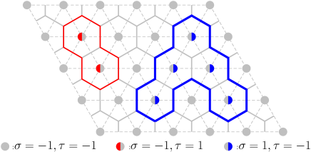
Figure 2: (Color online) A spin configuration of the AT model on the triangular lattice and the corresponding LT-expansion graph on the honeycomb lattice. Thick blue line represents blue bond; thin red line denotes red bond; the same below.

Instead of directly updating the spins, the worm-type algorithms worm1 ; worm2 for the Ising model simulate the graphical representation which can be the high- and the low-temperature expansion graphs. The worm methods in Refs. worm1 ; worm2 can be generalized to the graphical expansion of the AT model. In the following, we shall use the low-temperature (LT) expansion, defined on the dual lattice of the triangular lattice—the honeycomb lattice. Given a spin configuration $\{\sigma,\tau\}$, for each pair of nearest-neighboring vertices $(i,j)$, one places on its dual edge:

• nothing if $\sigma_{i}=\sigma_{j},\tau_{i}=\tau_{j}$,

• a red occupied bond if $\sigma_{i}=\sigma_{j},\tau_{i}\neq\tau_{j}$,

• a blue occupied bond if $\sigma_{i}\neq\sigma_{j},\tau_{i}=\tau_{j}$,

• a red and a blue bond if $\sigma_{i}\neq\sigma_{j},\tau_{i}\neq\tau_{j}$.

In other words, depending on the associated pair of spins on the triangular lattice, an edge on the honeycomb lattice can be in one of the four states: vacant, red, blue, and red+blue. An example is shown in Fig. 2. Since the coordination number is 3 for the honeycomb lattice, the red and blue bonds form a series of disjointed loops in red and blue color, respectively. Note that the red and the blue loops are allowed to share common edges. In this way, a spin configuration on the triangular lattice is mapped onto a loop configuration on the honeycomb lattice, while a loop configuration corresponds to 4 spin configurations , which are related to each other by globally flipping the $\sigma$ or/and $\tau$ Ising spins. Let $|E_{r}|$, $|E_{b}|$, and $|E_{r+b}|$ be the number of red, blue, and red$+$blue bonds, the partition sum of the AT model can be written as (up to an unimportant factor)

$$\mathcal{Z}_{\rm AT}=\sum_{\{\mathcal{L}\}}X_{r}^{|E_{r}|}X_{b}^{|E_{b}|}X_{r+b}^{|E_{r+b}|}\;,$$ (3)

where the summation $\{\mathcal{L}\}$ is over all loop configurations. From the mapping, one can obtain the relative statistical weights as

$$X_{r}=X_{b}=e^{-2J-2K}\mbox{ and }X_{r+b}=e^{-4J}\;.$$ (4)

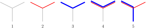
Figure 3: (Color online) Vertex states in the LT-expansion graph of the AT model.

One can further describe the AT model in the language of the vertex states, which will serve as the basis for the formulation of the worm-type algorithms in this work. In the loop configurations, all the vertices must have an even number of incident red (blue) bonds. Accordingly, only the 5 types of vertex states in Fig. 3 exist, where the states are unchanged under spatial rotations. Simple calculations yield the statistical weights as

$$W_{1} = 1\;,\hskip 36.98857ptW_{2}=W_{3}=e^{-2J-2K}\;,$$

$$W_{4} = e^{-4J}\;,\mbox{ and }W_{5}=e^{-4J-2K}\;.$$ (5)

Let $|V_{i}|$ be the number of vertices at state $i$ with $i=1,2,3,4,5$, the partition sum of the AT model can be written as (up to a constant)

$$\mathcal{Z}_{\rm AT}=\sum_{\{\mathcal{V}\}}\prod_{i=1}^{5}W_{i}^{|V_{i}|}\;,$$ (6)

where the summation $\{\mathcal{V}\}$ is over configurations with vertex states in Fig. 3.

II.2 Exact mapping in the $J\rightarrow-\infty$ limit

Given a finite four-spin coupling $K$, when the antiferromagnetic coupling $J$ becomes stronger and stronger, more and more vertices will be at state-4 and -5 in Fig. 3, because $W_{4}\sim W_{5}\propto\exp(-4J)$ increases faster than $W_{1},W_{2},W_{3}$, as seen from Eq. (5). In the $J\rightarrow-\infty$ limit, only state-4 and -5 survive. We can then redefine the edge states in state-4 and -5 as following. The empty edge is replaced by a ‘dimer’, while the ‘blue+red’ edge is regarded as empty; namely, the edge is now at state: empty, dimer, red, or blue. As a result, state-4 and -5 become those in Fig. 4(a).

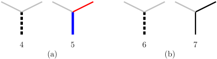
Figure 4: (Color online) (a), State-4 and -5 after the redefinition of the edge states. (b), Vertex states in the FPLD model. The dashed black line represents dimer.

One observes that the occupied bonds at state-5 form a series of disjointed loops; these loops are now constructed by bonds alternatively in color red and blue. Further, one notes that the color-degree freedom can be simply integrated out, and each loop gains a statistical-weight factor 2. Without the color information, the edge is at state: empty, dimer, or bond, and the vertex states reduce to those in Fig. 4(b), where new labels ‘6’ and ‘7’ are used. The statistical weights are

$$W_{6}=1\;,\hskip 17.07164ptW_{7}=e^{-2K}\;.$$ (7)

On this basis, the partition sum of the AT model in the $J\rightarrow-\infty$ limit can be written as

$$\mathcal{Z}_{\rm FPLD}=\sum_{\{\mathcal{V}\}}n^{\ell}W_{7}^{|V_{7}|}\;,\hskip 17.07164pt(n=2)$$ (8)

where the summation is over configurations with all vertex states in Fig. 4, and $\ell$ is the number of loops. We shall refer to the model defined by Eq. (8) and Fig. 4 as the $n$-color FPLD model.

Note that, for finite $K$, the loops in the FPLD model are ‘dilute’ due to the presence of state-6. However, in the $K\rightarrow-\infty$ limit, only state-7 survives, and one obtains the mapping between the triangular 4-state antiferromagnet at zero temperature and the honeycomb $n=2$ fully-packed loop model. For $K\rightarrow\infty$, the model reduces to the fully-packed dimer model, which is equivalent to the triangular Ising antiferromagnet at zero temperature.

We conclude this subsection by mentioning that the FPLD model is very similar to the honeycomb O$(n)$ loop model Nienhuis . The difference is that in the former the vertices off the loops are paired up by dimers, while not in the latter. Namely, the configuration space for the FPLD model is a subspace in the O$(n)$ loop model. Albeit it remains to be explored whether or not the two models are in the same universality class, it is not surprising if this turns out to be the case.

III Worm Algorithms

The worm algorithm for the high-temperature expansion graphs of the Ising model was first formulated by Prokof’ev and Svistunov worm1 , and the dynamic critical behavior was studied in Ref. worm2 . Recently, Wolff provided a worm-type simulation strategy for O(N) sigma/loop models wolff . The underlying physical picture of the worm method is beautifully simple: enlarge the state space of the to-be-simulated model, define an extended model, and simulate the system by a local algorithm.

III.1 Worm algorithm for finite $J$

Let us now generalize the worm method in Refs. worm1 ; worm2 to the AT model in the language of the vertex states, defined by Eq. (6) and Fig. 3.

Enlarge the state space. We first introduce new vertex states by deleting from (or adding to) the states in Fig. 3 a red or blue bond. This leads to the 8 additional vertex states in Fig. 5.

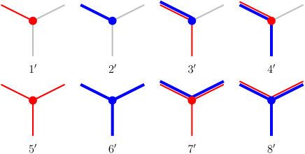
Figure 5: (Color online) Additional vertex states in the worm method for the AT model. The red (blue) filled circle denotes a defect in red (blue) vertex configuration.

The state space is then enlarged such that a configuration has a pair or none of vertices at states in Fig. 5. Such a pair of vertices are named ‘defects’ and denoted as $(u,v)$. Accordingly, the state space can be divided into two subspaces: one without defect ($u=v$) and the other with two defects ($u\neq v$); we shall refer to them the M (measuring) and W (worm) sector, respectively. A careful check yields that the pair of defects in the W sector must be connected via a string of red or blue occupied bonds. Namely, $u$ and $v$ are either both at states $\{1^{\prime},4^{\prime},5^{\prime},7^{\prime}\}$ or $\{2^{\prime},3^{\prime},6^{\prime},8^{\prime}\}$ in Fig. 5. For the later convenience, we let $u,v$ be ordered as $u\leftarrow v$, and thus the interchange $(u\leftrightarrow v)$ would lead to a different configuration for $u\neq v$.

Define the extended model. With the inclusion of the defects and the vertex states in the W sector, a configuration can now be completely specified by its vertex states $\{\mathcal{V}\}$, and the ordered pair of defects $(u,v)$. The partition sum of the extended model can be separated into two parts. The part in the M sector is defined as

$$\mathcal{Z}_{M}=\mathcal{Z}_{\rm AT}=\frac{1}{V}\sum_{\{\mathcal{V},u,v\}}\delta_{u=v}\prod_{i=1}^{5}W_{i}^{|V_{i}|}\;,$$ (9)

where $V$ is the volume of the system and $\delta$ is the Kronecker delta function. The summation $\{\mathcal{V}\}$ is over vertex-state configurations with states in Fig. 3 and coordinations $(u,v)$. Factor $1/V$ accounts for the summation of $u=v$ over the whole lattice. Similarly, the part of the partition sum in the W sector can be defined by

$$\mathcal{Z}_{W}=\frac{1}{V}\sum_{\{\mathcal{V},u,v\}}\delta_{u\neq v}\prod_{i=1}^{5}W_{i}^{|V_{i}|}\prod_{j=1}^{8}W_{j^{\prime}}^{|V_{j^{\prime}}|}\;,$$ (10)

where the summation $\{\mathcal{V}\}$ is over configurations with two vertex states in Fig. 5 and all other in Fig. 3, and $W_{j^{\prime}}$ are the statistical weights for states in Fig. 5. The extended model can then be defined as

$$\mathcal{Z}_{\rm worm}=\mathcal{Z}_{M}+\xi_{w}\mathcal{Z}_{W}\;,$$ (11)

with $\xi_{w}>0$ a constant factor controlling the relative weight in the M and the W sector.

For a complete definition of the extended model, the statistical weights $W_{j^{\prime}}$ for states in Fig. 5 should have a definite value. It is natural that they are defined in accordance with the edge states, which lead to

$$W_{1^{\prime}}=W_{2^{\prime}} = e^{-J-K}\;,\hskip 8.53581ptW_{3^{\prime}}=W_{4^{\prime}}=e^{-3J-K}\;,$$

$$W_{5^{\prime}}=W_{6^{\prime}} = e^{-3J-3K}\;,W_{7^{\prime}}=W_{8^{\prime}}=e^{-5J-K}\;.$$ (12)

Formulate the worm algorithm. One can now use any valid algorithm to simulate the model defined by Eq. (11). Since a configuration is specified by the ordered triplet of parameters $(\mathcal{V},u,v)$, an update can be acted on the vertex states $\mathcal{V}$ and/or the locations of defects $(u,v)$. The worm strategy is to randomly move $u$ and/or $v$ around the lattice and update $\mathcal{V}$ by changing the edge states during the biased random walk. Suppose that $u\neq v$ are in red (in the W sector). As $u$ moves to a neighboring vertex $u_{n}$, the edge $(uu_{n})$ state will be symmetrically updated: a red bond is placed (deleted) if it is absent (present). In this way, state at $u$ will be back in Fig. 3 after $u$ moves $u_{n}$. Accordingly, the number of defects remains unchanged if $v\neq u_{n}$ or becomes zero if $v=u_{n}$. This accounts for a step of random walk in the W sector or from the W to the M sector. For the case $u=v$, by the symmetric update of edge state, one will generate a pair of defects which can be either in red or blue. Therefore, one never introduces more than two defects. The parameter $\xi=1$ is set in this work, and a version of the worm algorithm reads (Algorithm 1)

1. If $u=v$, randomly choose a new vertex $u^{\prime}$ and set $u=v=u^{\prime}$. Equally choose color red or blue for the to-be-proposed defects; say red.

2. Interchange $u\leftrightarrow v$ with probability $1/2$.

3. Randomly choose one neighboring vertex $u_{n}$ of $u$. Propose to move $u\rightarrow u_{n}$.

4. Propose to symmetrically update the edge-$uu_{n}$ state: red $\leftrightarrow$ vacant and blue $\leftrightarrow$ red+blue.

5. Accept the proposal with probability

   $$\mathcal{P}_{a}=\min\left[1,(W^{(a)}_{u}W^{(a)}_{u_{n}})/(W^{(b)}_{u}W^{(b)}_{u_{n}})\right]\;,$$

   according to the Metropolis-Hasting scheme. The superscript $(b)$ and $(a)$ means “before” and “after update”, respectively. The statistical weights are given Eqs. (5) and (12).

Monte Carlo simulation of the AT model consists of repetition of these steps. The detailed balance at each step is straightforward since the algorithm is just a Metropolis-type update. If one regards the connected pair of ‘defects’ as a worm, the above steps mimic the crawling of the worm on the lattice. This is responsible for the terminology ‘worm’.

Measurement. Measurement can take place either in the whole enlarged state space or in the M subspace. For the high-temperature graph of the Ising model, it can be shown that the partition sum of the extended model is related to the Ising model as $\mathcal{Z}_{\rm worm}=\chi\mathcal{Z}_{\rm Ising}$, where $\chi$ is the magnetic susceptibility. Thermodynamic quantities can be measured in the enlarged configuration space. Nevertheless, if one is only interested in the original system, it is sufficient to sample in the M sector. This would define a Markov subchain with a coarse unit of Monte Carlo step between two subsequent configurations in the M sector. The detailed balance is clear since it is satisfied in each basic step in Algorithm 1.

Improved version. As mentioned earlier, state-4 and -5 (Fig. 3) would dominate in the M sector as $J\rightarrow-\infty$; analogously, only state-$7^{\prime}$ and -$8^{\prime}$ (Fig. 5) survive in the limit, as seen from Eq. (12). This implies that, as soon as both $u$ and $v$ are at state-$7^{\prime}$ and $-8^{\prime}$, they will be frozen there forever, and thus Algorithm 1 becomes non-ergodic.

The same difficulty occurs for the worm simulation of the triangular Ising antiferromagnet at zero temperature. A rejection-free technique was introduced improved ; QQLiu to overcome such a problem, based on the observation that the detailed balance in the coarse step does not require the detailed balance in each basic step in the W sector. Let $u_{n}\;(n=1,2,3)$ denote the neighbouring vertices of $u$ and $p_{n}$ be the probability that $u$ moves to $u_{n}$ in Algorithm 1, the probability for $u$ to be unmoved is $p_{0}=1-(p_{1}+p_{2}+p_{3})$. The absorbing problem of $(u,v)$ at state-$7^{\prime}$ and -$8^{\prime}$ is reflected by $p_{0}\rightarrow 1$ as $J\rightarrow-\infty$. In the W sector, one can explicitly set zero for the probability that $u$ remains unmoved, and defines the new transition probabilities $p^{\prime}_{n}$ as

$$\frac{p^{\prime}_{1}}{p_{1}}=\frac{p^{\prime}_{2}}{p_{2}}=\frac{p^{\prime}_{3}}{p_{3}}\;,$$

$$p^{\prime}_{0}=1-(p^{\prime}_{1}+p^{\prime}_{2}+p^{\prime}_{3})=0\;.$$ (13)

The details can be found in Refs. improved ; QQLiu .

The absorbing problem can also be solved in the present formulation of the worm algorithm. Actually, the absorbing problem is somewhat ‘artificial’ here, since it arises from the particular assignment of the statistical weights to states in Fig. 5 by Eq. (12). There is no reason, however, why one should use Eq. (12) if only the original AT model (6) is of interest. The absorbing problem simply dissolves if the statistical weights are given by

$$W_{1^{\prime}}=W_{2^{\prime}} = e^{-2J-2K}\;,W_{3^{\prime}}=W_{4^{\prime}}=e^{-4J}\;,$$

$$W_{5^{\prime}}=W_{6^{\prime}} = e^{-2J-2K}\;,W_{7^{\prime}}=W_{8^{\prime}}=e^{-4J-2K}\;.$$ (14)

Other definitions are possible.

III.2 Worm algorithm for $J\rightarrow-\infty$

Algorithm 1 using Eq. (14) is found to be efficient in most of the region with $0>J>-\infty$ and for small $K$ in the $J\rightarrow-\infty$ limit. In this limit, the efficiency significantly drops as $K$ deviates from $0$.

Hereby we shall make use of the exact mapping of the AT model onto the FPLD model (8) and formulate another version of the worm algorithm. Following the same procedure in the above subsection, we first introduce 5 additional states in Fig. 6.

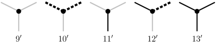
Figure 6: (Color online) Vertex states in the W sector for the FPLD model. The black filled circle denotes a defect.

The partition sum in the M sector is defined as

$$\mathcal{Z}_{M}=\mathcal{Z}_{\rm FPLD}=\frac{1}{V}\sum_{\{\mathcal{V},u,v\}}\delta_{u=v}n^{\ell}W_{7}^{|V_{7}|}\;,$$ (15)

with $n=2$. Again, the summation is over configurations with states in Fig. 4 and over the location of $u=v$. The partition sum in the W sector is given by

$$\mathcal{Z}_{W}=\frac{1}{V}\sum_{\{\mathcal{V},u,v\}}\delta_{u\neq v}n^{\ell}W_{7}^{|V_{7}|}\prod_{j=9}^{13}W_{j^{\prime}}^{|V_{j^{\prime}}|}\;.$$ (16)

The extended model is defined by Eq. (11).

The formulation of the worm algorithm follows the standard strategy in the above subsection, except that the edge-state update should take a different scheme. Let $e=0,1,2$ denote the edge-$e$ state ‘empty’, ‘bond’, and ‘dimer’, respectively, and define the module-3 summation rule as $\mod_{3}(e+\Delta e)$ with $\Delta e=1,2$. As moving $u\rightarrow u_{n}$, one randomly chooses $\Delta e=1$ or 2 and propose to update the edge-$uu_{n}$ state as $\mod_{3}(e+\Delta e)$. In other words, an ‘empty’ edge is proposed to randomly become a ‘bond’ or a ‘dimer’; ‘dimer’ is to be ‘empty’ or ‘bond’; and ‘bond’ is to be ‘empty’ or ‘dimer’. However, not all the proposals will generate a valid configuration that has at most two states in Fig. 6 and the others in Fig. 4. For instance, (1), in the M sector, when $u=v$ is at state-$7$ and the empty edge is proposed to become a dimer, the resulting vertex state at $u$ will not be in Fig. 6; (2), in the W sector, when $u$ is at state-$9^{\prime}$ and the proposal is $e=0\rightarrow e=1$, this would yield state-$11^{\prime}$ at $u$ which is not in Fig. 4 as required. A proposal would be rejected if it leads to an invalid configuration. On this basis, a version of the worm algorithm can be formulated as (Algorithm 2)

1. If $u=v$, move it to a randomly chosen vertex.

2. Same as in Algorithm 1.

3. Same as in Algorithm 1.

4. Randomly choose $\Delta e=1$ or $2$, and propose to update the edge-$uu_{n}$ state as $e_{uu_{n}}\rightarrow\mod_{3}(e_{uu_{n}}+\Delta e)$. The proposal will be rejected if it yields

   • for $u=v$, $V_{v}$ or $V_{u_{n}}$ $\not\in\{9^{\prime},\cdots,13^{\prime}\}$ in Fig. 6;

   • for $u\neq v$ and $v\neq u_{n}$, $V_{u}$ $\not\in\{6,7\}$ in Fig. 4 or $V_{u_{n}}$ $\not\in\{9^{\prime},\cdots,13^{\prime}\}$;

   • for $u\neq v$ and $v=u_{n}$, $V_{u}$ or $V_{u_{n}}$ $\not\in\{6,7\}$.

   In this case, step-5 will be skipped. Symbol $V_{u}$ represents the vertex state at $u$.

5. Accept the update with probability

   $$\mathcal{P}_{a}=\min\left[1,n^{\Delta_{\ell}}\;(W^{(a)}_{u}W^{(a)}_{u_{n}})/(W^{(b)}_{u}W^{(b)}_{u_{n}})\right]\;,$$

   where $\Delta\ell$ denotes the change of the loop number in the update. We remind that the constant $\xi_{w}$ in Eq. (11) is set $\xi_{w}=1$.

Simulation consists of repetition of these steps, and the measurement is taken in the M sector.

A practically important matter for implementing Algorithm 2 is that a non-local query is needed to calculate the loop-number difference $\Delta\ell$. We shall follow the simultaneous breadth-first searching technique and the trick to avoid as much as possible queries, as described in Ref. QQLiu .

More importantly, one can apply the so-called coloring method to avoid altogether the need for such global queries for $n\geq 1$. The key ingredient of the coloring method is the trivial identity $n=1+(n-1)$ for the statistical weight $n$ of each loop. One can introduce an auxiliary variable $c=0,1$ and rewrite the identity as

$$n=\sum_{c=0,1}[1\delta_{c,0}+(n-1)\delta_{c,1}]\;.$$ (17)

The variable $c$ is generally referred to as the coloring variable, and $c=0$ (1) is said ‘active’ (‘inactive’) . See Refs. QQLiu for details. In practise, the coloring variable is assigned to each vertex in the M sector as (Coloring assignment)

1. Set all vertices off loops be active ($c=0$).

2. Independently for each loop, choose $c=0$ with probability $1/n$ and $c=1$ with probability $(1-1/n)$, and assign it to all the vertices on the loop.

On the basis of the Coloring assignment, the whole lattice $G$ is divided into the active sublattice $G_{a}$ and the inactive sublattice $G_{i}$. In $G_{a}$ the vertices are active and the edges connect two active vertices; in $G_{i}$ the vertices are inactive and the edges connect two inactive vertices. The edges connecting one active and one inactive vertex form the boundaries separating $G_{a}$ and $G_{i}$. We state that, conditioning on this decomposition, the vertex-state configuration on the induced sublattice $G_{a}$ and $G_{i}$ is nothing but a generalized FPLD model with $n^{\prime}=1$ and $(n-1)$, respectively.

One has now the right to update these generalized FPLD models via any valid Monte Carlo algorithm. We choose Algorithm 2 to update the model with $n^{\prime}=1$ on $G_{a}$ and the identity operation (‘do nothing’) on $G_{i}$. Due to the fact $n^{\prime}=1$, the loop-number change $\Delta\ell$ does not matter anymore. Therefore, one can formulate another version of the worm algorithm as (Algorithm 3)

1. Do the Coloring assignment if $u=v$.

2. Do $M$ times of the coarse Monte Carlo steps (from and back to the M sector) by performing Algorithm 2 on the induced subgraph $G_{a}$ with $n^{\prime}=1$.

The parameter $M\geq 1$ can be set such that step 1 and 2 take comparable CPU time.

For the actual implementation of Algorithm 2 and 3, positive statistical weights have to be assigned to vertex states in Fig. 6. Before discussing on this, we mention that there exist some freedom to choose which vertex state is allowed in the W sector. As long as ergodicity is satisfied, the consideration is to optimize the efficiency. In Fig. 6, we do not allow the state with two bonds and a dimer, because the only way to generate this state is to add a dimer to state-$7$ and the only way to return to Fig. 4 is to delete the newly generated dimer. Thus, such a state will not help updating the configuration while increasing computational burden. In contrast, state-$9^{\prime}$ and -$10^{\prime}$ (-$11^{\prime}$ and -$13^{\prime}$) are important for moving around the dimers (bonds). We set

$$W_{9^{\prime}} = W_{10^{\prime}}=1\hskip 5.69054ptW_{12^{\prime}}=\min(1,W_{7})\hskip 5.69054pt\mbox{ and}$$

$$W_{11^{\prime}} = W_{13^{\prime}}=W_{7}\;\;=e^{-2K}\;.$$ (18)

State-$12^{\prime}$ is useful for switching between dimer and bond, but should not occur more frequently than state-6 or -7.

IV Results

The complete phase diagram of AT model on the triangular lattice is shown in Fig. 7. In following, we shall present numerical results and discuss the phase boundary in the antiferromagnetic two-spin coupling region ($J<0$).

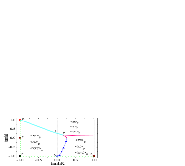
Figure 7: (Color online) Phase diagram of the AT model on the triangular lattice. Points–‘P’, ‘I’, ‘O’–correspond to the 4-state Potts, the Ising, and the O(2) loop model, respectively. Points–‘F’, ‘C’, ‘D’–denote the zero-temperature Ising antiferromagnet in variable $\sigma\tau$, $\sigma$ or $\tau$ (decoupled), $\sigma$ or $\tau$ (correlated), respectively. Point ‘E’ is the zero-temperature 4-state Potts antiferromagnet.

IV.1 Finite $J$

We employ Algorithm 1 with Eq. (14) to simulate the AT model in the region of finite $J<0$ on triangular lattices with periodic boundary conditions, using system sizes in the range $6\leq L\leq 192$.

For a given loop configuration, we generate the associated spin configuration on the triangular lattice according to the low-temperature expansion rule. Note that, due to the periodic boundary condition, a loop configuration may correspond to no spin configuration. This occurs when there exists an odd number of red or blue loops winding around the boundary. In this case, we take no measurement, and the simulation continues until the next try. Let $X$ be the indicator function which is $1$ if the loop configuration is measuring and corresponds to a spin configuration, and $0$ otherwise; let $\mathcal{O}$ be the operator computed in one of the $4$ compatible spin configurations; therefore, what we are computing is $[\mathcal{O}X]/[X]$, with $[\;]$ the statistical average over loop configurations. The non-valid loop configuration is not weighted, thus it does not influence any of the numerical data related to the spin variables. Further, since the special cases that the loop configuration does not correspond to any spin configuration result from boundary effects, such cases do not dominate in large systems.

Two types of magnetization are measured as

$$M_{\sigma}=\frac{1}{V}\sum_{i}\sigma_{i}\hskip 14.22636pt\mbox{and}\hskip 14.22636ptM_{\sigma\tau}=\frac{1}{V}\sum_{i}\sigma_{i}\tau_{i}\;,$$ (19)

where the summation is over the whole lattice. Accordingly, the susceptibilities are defined as

$$\chi_{\sigma}=V\langle M_{\sigma}^{2}\rangle\hskip 14.22636pt\mbox{and}\hskip 14.22636pt\chi_{\sigma\tau}=V\langle M_{\sigma\tau}^{2}\rangle\;,$$ (20)

with $\langle\;\rangle$ for statistical average. Dimensionless ratios are found to be very powerful in locating the critical points of many systems under continuous phase transitions. On the basis of the fluctuation of the magnetization, we define two distinct dimensionless ratios as  binder

$$Q_{\sigma}=\frac{\langle M_{\sigma}^{2}\rangle^{2}}{\langle M_{\sigma}^{4}\rangle}\hskip 8.53581pt\mbox{and}\hskip 8.53581ptQ_{\sigma\tau}=\frac{\langle M_{\sigma\tau}^{2}\rangle^{2}}{\langle M_{\sigma\tau}^{4}\rangle}\;.$$ (21)

We also measure energy-like quantities as

$$E_{\sigma} = -J\sum_{\langle i,j\rangle}\sigma_{i}\sigma_{j}$$ (22)

$$E_{\sigma\tau} = -K\sum_{\langle i,j\rangle}\sigma_{i}\tau_{i}\sigma_{j}\tau_{j}$$ (23)

$$E = E_{\sigma}+E_{\tau}+E_{\sigma\tau}\;,$$ (24)

as well as the associated specific-heat-like quantities $C_{\sigma}=(\langle E_{\sigma}^{2}\rangle-\langle E_{\sigma}\rangle^{2})/V$, $C_{\sigma\tau}$, and $C$.

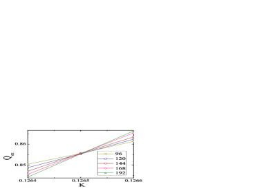
Figure 8: (Color online) Quantity $Q_{\sigma\tau}$ versus $K$ at $J=-1.0$. Lines connecting the data points are for illustration purpose.

The AT model for $J=0$ reduces to the standard Ising model in the Ising-spin variable $\sigma\tau$, and undergoes a Ising-like transition at $K_{c}$. For $K<K_{c}$, the configurations in the Ising variables $\sigma$, $\tau$, and $\sigma\tau$ are all in the disordered (paramagnetic) state; for $K>K_{c}$, $\sigma\tau$ is in the ferromagnetic state while $\sigma$ and $\tau$ are still in the paramagnetic state. We expect that this scenario continues into the region $J<0$.

We choose $J=-0.2,-0.6,-1.0$, and $-2.0$, and perform some preliminary and coarse simulations to approximately locate the intersection of $Q_{\sigma\tau}$ for various linear system sizes $L$. Then, fine and extensive simulations are carried out near the estimated critical point. Figure 8 displays $Q_{\sigma\tau}$ versus $K$ for different $L$ at $J=-1.0$, indicating a critical point near $K\approx 0.1265$.

The finite-size scaling behavior of $Q_{\sigma\tau}(K,L)$ near the critical point $K_{c}$ is described by

$$Q(K,L)=Q(tL^{y_{t}},bL^{y_{i}})\;,$$ (25)

where $t$ and $i$ represent the leading and the subleading thermal scaling fields, with $t\propto(K-K_{c})+\cdots$. The associated renormalization exponents are denoted as $y_{t}$ and $y_{i}$. A Taylor expansion of Eq. (25) yields Deng

$$Q(K,L) = Q_{c}+a_{1}\Delta KL^{y_{t}}+a_{2}(\Delta K)^{2}L^{2y_{t}}+bL^{y_{i}}$$ (26)

$$+ c\Delta KL^{y_{t}+y_{i}}+...\;,$$

with $\Delta K\equiv K-K_{c}$. Parameters $a_{1}$, $a_{2}$, $b$, and $c$ are unknown constants.

According to the least-squares criterion, we fit the $Q_{\sigma\tau}$ data to Eq. (26). Assuming the transition is Ising-like, we expect that the leading two finite-size correction exponents are $y_{1}=2-2y_{h}=-7/4$ and $y_{2}=y_{i}=-2$ for $Q_{\sigma\tau}$, where $y_{h}=15/8$ is the magnetic renormalization exponent. With $y_{1}$ and $y_{2}$ fixed and $L\geq L_{\rm min}=48$, we obtain $K_{c}=0.12653(2)$, $y_{t}=1.01(2)$, and $Q_{c}=0.8587(1)$ for $J=-1.0$. The chi square per degree of freedom ($\bar{\chi}^{2}$/dof) is 1.14. The estimate of $y_{t}$ is consistent with the exact result $y_{t}=1$, and the universal ratio $Q_{c}=0.8587$ also agrees well with the earlier estimate $Q_{c}=0.858\,725\,28(3)$ for the Ising model on the triangular lattice blote1 .

The data of susceptibility $\chi_{\sigma\tau}$ is analyzed by

$$\chi(K,L) = L^{-2y_{h}+d}(a_{0}+a_{1}\Delta KL^{y_{t}}+a_{2}(\Delta K)^{2}L^{2y_{t}}$$ (27)

$$+ bL^{y_{i}}+c\Delta KL^{y_{t}+y_{i}}+...)\;,$$

and we determine the magnetic exponent as $y_{h}=1.876(2)$, in good agreement with the exact value $y_{h}=15/8$. The specific-heat-like quantity $C$ is also found to diverge approximately in the logarithmic scale as $L$ increases. No phase transition is observed for Ising variable $\sigma$ or $\tau$.

Similar results are found for other values of $J$, and the estimated critical points are listed in Table 1.

$J$	-0.2	-0.6	-1.0	-2.0
$K_{c}$	$0.25303\,(2)$	$0.18164\,(2)$	$0.12653\,(2)$	$0.06306\,(3)$
$L_{\rm min}$	48	48	48	48
$\bar{\chi}^{2}$/dof	1.05	0.86	1.14	1.21

Table 1: Details in the data fits according to Eq. 26.

On this basis, we conclude that the phase transition of the AT model in region $(K>0,J<0)$ with finite $J$ is in the Ising universality. Finally, we mention that the worm-type algorithm hereby does not suffer much from critical slowing-down.

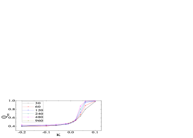
Figure 9: (Color online) Dimensionless ratio $Q_{\sigma\tau}$ versus $K$ for the n=2 FPLD model.

IV.2 $J\rightarrow-\infty$

Table 1 suggests that the critical coupling $K_{c}$ becomes smaller as $J$ becomes more negative, and that the ending point of the critical line for $J\rightarrow-\infty$ is very close to $K=0$, since $K_{c}(J=-2)=0.06306(3)$ is already near $0$. To locate the ending point more accurately, we directly simulate the $J\rightarrow-\infty$ limit, which makes use of the exact mapping to the $n=2$ FPLD model and employs Algorithm 3. System sizes take $6$ values in range $30\leq L\leq 960$.

Note that the loops in the FPLD model serve as domain walls for the Ising variable $\sigma\tau$ in the AT model. According to the low-temperature expansion rule, on the triangular lattice we sample magnetization density $M_{\sigma\tau}$, susceptibility $\chi_{\sigma\tau}$, dimensionless ratio $Q_{\sigma\tau}$, energy $E_{\sigma\tau}$, and specific heat $C_{\sigma\tau}$, whose definitions can be found in Eqs. (19)–(24). Further, to explore the loop-length distribution, on the honeycomb lattice we measure the length of the longest loop as $S_{1}$.

The finite-size data of the dimensionless ratio $Q_{\sigma\tau}$ are plotted in Fig. 9; an eye-view fitting yields a critical point as $K_{c}=0.00(2)$. For $K>K_{c}$, the $Q_{\sigma\tau}$ value rapidly approaches to $1$ as size $L$ increases. This reflects that the Ising variable $\sigma\tau$ exhibits a long-range ferromagnetic order on the triangular lattice; correspondingly, on the honeycomb lattice loops are small–i.e., in a disordered state. For $K<K_{c}$, $Q_{\sigma\tau}$ converges to a constant $Q_{c}$ which deviates from the trivial Gaussian value $1/3$. This implies that, despite the absence of a long-range order, the spin-spin correlation function decays algebraically over the distance.

In Fig. 9, one can observe that $Q_{\sigma\tau}$ at $K<0$ rapidly converges to a K-dependent value, as expected in the low-temperature BKT phase. This reminds us the analogy between the FPLD and Nienhuis’s O$(n)$ honeycomb loop model with $n=2$. The phase diagram of the latter is shown in Fig. 10, where $x$ is the statistical weight for an occupied bond. For a given $0\leq n\leq 2$, the O$(n)$ loop model exhibits three distinct phases: a dilute and disordered phase (small $x$), a densely-packed phase (large finite $x$), and a fully-packed phase (infinite $x$). Furthermore, the model is exactly solvable on the curves Nienhuis

$$\frac{1}{x_{\pm}}=\sqrt{2\pm\sqrt{2-n}}\;.$$ (28)

The system is equivalent to the tricritical $q=n^{2}$ Potts model along the critical line $x_{+}$, belongs to the critical $q=n^{2}$ Potts universality class in the densely-packed phase, and is in another critical universality in the fully-packed phase. For $n=2$, the two solvable lines $x_{\pm}$ merge at a single point; the renormalization field is marginally relevant (irrelevant) for $x<x_{\pm}$ ($x>x_{\pm}$). In other words, the phase transition at $x_{\pm}$ is Berezinsky-Kosterlitz-Thouless(BKT)-like. At the special point $x_{\pm}(n=2)$, the amplitude of the renormalization field is zero, and thus logarithmic corrections, present at most of BKT-like critical points, disappear. This explains the absence of logarithmic corrections in the critical Baxter-Wu model, which can be exactly mapped onto the O(2) loop model at $x_{\pm}$. For the critical O(2) loop model, it has been identified that $S_{1}\propto L^{y_{H}}=L^{3/2}$ and $\chi_{\sigma\tau}\propto L^{2y_{t0}-2}=L$, where $y_{H}=3/2$ is the hull exponent and $y_{t0}=3/2$ is the leading thermal renormalization exponent in the language of the Potts model dengy07 .

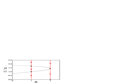
Figure 10: (Color online) Phase diagram of the O(n) loop model Nienhuis . Red lines denote the directions of the renormalization flows.

Since the state space of the FPLD model is a subspace of the O(2) loop model, it is reasonable to conjecture that the two models are in the same universality class. Namely, we expect that the FPLD model undergoes a BKT-like transition at $K_{c}$, where the logarithmic corrections are absent; for $K<K_{c}$ the system is in the same universality class as at $K_{c}$ but with logarithmic corrections; for $K\rightarrow-\infty$ it is in another universality class. Making use of the known exponent $y_{H}=3/2$ for $S_{1}$ and $2y_{t0}-2=1$ for $\chi_{\sigma\tau}$, we plot $L^{-3/2}S_{1}$ and $L^{-1}\chi_{\sigma\tau}$ versus $K$ in Figs. 11 and 12, respectively. They both display a nice intersection at $K=0.000$. From Fig. 12 one can observe that the exponent $y_{H}$ varies along the BKT critical line, which reconciles the difference of $y_{H}$ between the present model and the two-dimensional XY models.

Figure 11: (Color online) $L^{-3/2}S_{1}$ versus $K$ for the n=2 FPLD model.

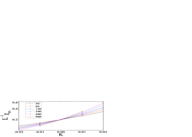
Figure 12: (Color online) $L^{-1}\chi_{\sigma\tau}$ versus $K$ for the n=2 FPLD model.

To further explore the potential logarithmic corrections, we assume $K_{c}=0$ and plot $L^{-3/2}S_{1}$ and $L^{-1}\chi_{\sigma\tau}$ at $K=0$ versus $L^{-1}$. As shown in Fig. 13, the rapid convergence implies the absence of logarithmic corrections; corrections with term $L^{-1}$ are also very weak if they exist.

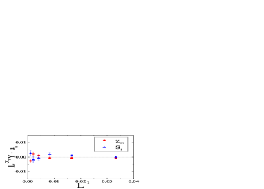
Figure 13: (Color online) Quantities $L^{-3/2}S_{1}-a_{0,s_{1}}$ and $L^{-1}\chi_{\sigma\tau}-a_{0,\chi}$ at $K=0$ versus $L^{-1}$ for the n=2 FPLD model. Constants $a_{0,s_{1}}$ and $a_{0,\chi}$ are obtained from the fits.

According to the least-squares criterion, the $S_{1}$ and $\chi_{\sigma\tau}$ data are fitted by

$$Y(K,L)=c_{0}+c_{1}\Delta K+\cdots+L^{X_{Y}}(a_{0}+a_{1}\Delta K\ln L$$

$$+a_{2}(\Delta K)^{2}\ln^{2}L+b_{1}L^{y_{1}}+b_{2}L^{y_{2}}+...)\;.$$ (29)

Here $a_{i}$ are coefficients of the finite-size scaling variable $\Delta K\ln L$ with $\Delta K=K-K_{c}$, $b_{i}$ are amplitudes of finite-size corrections, and the terms with $c_{i}$ accounts for analytical background. There are also cross-terms involving products of terms arising from these three sources. The exponent $X_{Y}$ is a general label for quantity $Y$. Equation (29) has assumed the absence of logarithmic corrections. It occurs that both the $S_{1}$ and the $\chi_{\sigma\tau}$ data with $L\geq L_{\rm min}=60$ can be well described by Eq. (29) with fixed correction exponents $y_{1}=-1$ and $y_{2}=-2$. The results for $S_{1}$ are $X_{Y}=1.498(3)$, $K_{c}=0.001(2)$, and $\bar{\chi}^{2}$/dof=1.22; for $\chi_{\sigma\tau}$ are $X_{Y}=1.001(2)$, $K_{c}=-0.001(1)$, and $\bar{\chi}^{2}$/dof=0.87. These agree well with the known exponents $3/2$ for $S_{1}$ and $1$ for $\chi_{\sigma\tau}$, as well as with the expectation $K_{c}=0$. If the exponents $X_{Y}$ are further fixed at the known values, we obtain $K_{c}=0.0002(3)$, $\bar{\chi}^{2}$/dof=0.94 from $S_{1}$ and $-0.0003(4)$, $\bar{\chi}^{2}$/dof=1.09 from $\chi_{\sigma\tau}$. On this basis, we estimate the critical point as $K_{c}=-0.0001(6)$, which covers the uncertainties of $K_{c}$ from $S_{1}$ and $\chi_{\sigma\tau}$.

We mention that, when an external field of strength $h/T$ is applied to the triangular Ising antiferromagnet, the critical state of the system is not immediately destroyed. Instead, the system has a BKT-like transition at $h_{c}=0.266(10)$  blote2 . However, our Monte Carlo results suggest that a critical point $K_{c}\neq 0$ is rather unlikely for the $n=2$ FPLD model.

In the limit $K\rightarrow\infty$, the Ising variable $\sigma\tau$ is in the ferromagnetic state. However, in terms of the $\sigma$ or the $\tau$ variable, it can be easily derived that the system is also an Ising model with coupling $2J$. Namely, along the $\tanh K=1$ line, the AT model has an Ising-like transition at $\tanh 2J=\sqrt{2}-1$. Further, the corner point ${\rm D}:\equiv(\tanh K=1,\tanh J=-1)$ corresponds to the triangular antiferromagnet at zero temperature, which is critical. Together with the earlier discussions in Sec. I, this means that, in Fig. 7, the limiting points–D, C, O, F, E–are all critical. From our simulations in range $-0.2\leq K\leq 0.1$ along the $\tanh J=-1$ line (EC+CD), we observe that, in the whole range, there exist algebraically decaying two-point correlation function for the $\sigma$ or the $\tau$ variable. On this basis, we conjecture that the whole $\tanh J=-1$ line (EC+CD) is critical for the $\sigma$ or the $\tau$ variable. Simulation along the $\tanh K=-1$ line using the present worm algorithms suffers significantly from critical slowing-down. Nevertheless, we suspect that the whole $\tanh K=-1$ line is critical for the $\sigma\tau$ variable.

V Dynamic Critical Behavior

In this section, we briefly report the efficiency of Algorithm 2 for the $n=2$ FPLD model, using the standard procedure described in Ref. SokalLectures .

For each observable (say $\mathcal{O}$), we calculate its autocorrelation function

$$\rho_{\mathcal{O}}(t)=\langle\mathcal{O}(t)\mathcal{O}(0)\rangle-\langle\mathcal{O}\rangle^{2},$$

where $\langle$ $\rangle$ denotes expectation with respect to the stationary distribution. We then obtain the corresponding integrated autocorrelation time as

$$\tau_{{\rm int},\mathcal{O}}=\frac{1}{2}\,\sum_{t=-\infty}^{\infty}\rho_{\mathcal{O}}(t)\;.$$ (30)

The dynamic critical exponent $z_{{\rm int},\mathcal{O}}$ is defined by

$$\tau_{{\rm int},\mathcal{O}}\sim\xi^{z_{{\rm int},\mathcal{O}}}.$$ (31)

where $\xi$ is the spatial correlation length. On a finite lattice at criticality, $\xi$ is cut off by system size $L$. Therefore, one has

$$\tau_{{\rm int},\mathcal{O}}=a+bL^{z_{{\rm int},\mathcal{O}}},$$ (32)

with $a$ and $b$ unknown parameters.

We simulate at the critical point $K_{c}=0$. Note that, during the worm simulations we measure the observables only when the chain visits the Eulerian subspace, roughly every $T_{E}\sim L^{d-2X_{e}}$ hits. However, it is natural to define $z_{\text{int},\mathcal{O}}$ as in Ref. improved to measure time in units of sweeps of the lattice, i.e. $L^{d}$ hits. Since one sweep takes of order $L^{2X_{e}}$ visits to the Eulerian subspace, we have $\tau\sim L^{z+2X_{e}}$. As shown in Fig.14, the exponent $2X_{e}$ is estimated to be $0.50(1)$.

Among the measured quantities including the longest-loop length $S_{1}$, the loop number $\ell$, and the energy-like quantity $E_{\sigma\tau}$ etc, $E_{\sigma\tau}$ is found to have the largest value of $\tau_{\rm int}$. Figure 15 displays $\rho_{E_{\sigma\tau}}(t/\tau_{{\rm int},E_{\sigma\tau}})$ as a function of $t/\tau_{int,E_{\sigma\tau}}$, where an approximately exponential decay is observed. The $\tau_{int,E_{\sigma\tau}}$ data are analyzed, and we obtain $z_{{\rm int},E_{\sigma\tau}}=0.28(1)$, which is shown in Fig. 16. Similar fits are done for other quantities, and we have $z_{{\rm int},S_{1}}=0.26(1)$ and $z_{{\rm int},\ell}=0.27(1)$. In these fits, $\bar{\chi}^{2}$/dof ranges from $0.74$ to $1.31$. Therefore, our numerical results suggest that the present worm algorithm is even more efficient than the one in Ref. improved .

Figure 14: (Color online) Ln($T_{E}/L^{2}$) versus lnL at $K=0$.

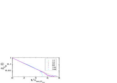
Figure 15: (Color online) $\rho_{E_{\sigma\tau}}(t/\tau_{int,E_{\sigma\tau}})$ versus $t/\tau_{{\rm int},E_{\sigma\tau}}$ at $K=0$.

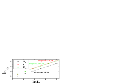
Figure 16: (Color online) Ln$(\tau_{{\rm int},\mathcal{O}})$ versus lnL for different observables at $K=0$.

Simulations are also carried out for $K=-0.05$, and the dynamic critical behavior cannot be distinguished from that for $K=0$.

VI Discussion

In summary, we have formulated two versions of the worm-type algorithms for the AT model on the triangular lattice. The algorithms are based on the low-temperature expansion graph of the AT model, and use the language of vertex states. Such a formulation not only provides us a different angle to understand the worm method, but also offers an easy way to overcome the absorbing difficulty. The efficiency of our algorithm is studied and can also be reflected by the fact that we can simulate up to size $L=960$. Apparently, Algorithm 1 can be applied to the ferromagnetic region $J>0$ of the triangular AT model and to the AT model on other planar lattices. Further, we mention that the worm-type algorithms can be developed on the basis of the high-temperature expansion graph of the AT model. This yields a graphical model also by Eq. (3), but defined on the original lattice for the AT model. The statistical weights of the occupied bonds are

$$X_{r} = X_{b}=(e^{2K}\sinh 2J)/(e^{2K}\cosh 2J+1)$$

$$X_{r+b} = (e^{2K}\cosh 2J-1)/(e^{2K}\cosh 2J+1)\;.$$ (33)

It is reasonable to expect good efficiency for the AT model on non-planar lattices–e.g., in higher spatial dimensions–with non-negative weights $X_{r}=X_{b}$ and $X_{r+b}$.

The high efficiency of the worm algorithms allows us to explore the triangular-lattice AT model in the antiferromagnetic region, and accordingly we conjecture a complete phase diagram in the $(J,K)$ plane. Of the particular interest is the $J\rightarrow-\infty$ limit, where the AT model is mapped onto the FPLD model with $n=2$. As suggested by the Monte Carlo simulation, the AT model undergoes a BKT-like transition along the $\tanh J=-1$ line, in the same universality class as the classical $XY$ model. We also mention that it remains to be explored whether or not, for other values of $n$, the FPLD and Nienhuis’s O$(n)$ model are in the same universality class.

Finally, we perform simulations for the AT model on the kaǵome lattice in the region $(J<0,K\geq 0)$, and determine a line of Ising-like critical points. The results are shown in Table 2. Unlike on the triangular lattice, the critical line ends at $K_{c}=0.3655>0$, still in the Ising universality. Taking into account that the frustration on the kaǵome lattice is only partial, this is not surprising. Accordingly, the phase diagram is shown in Fig. 17.

$J$	-0.2	-0.4	-0.6	-1.0	-2.0	$-\infty$
$K_{c}$	$0.442(2)$	$0.408(2)$	$0.386(2)$	$0.370(2)$	$0.366(2)$	0.3655(3)
$L_{min}$	36	36	36	36	36	36
$\bar{\chi}^{2}$/dof	1.21	0.91	1.07	1.23	0.85	1.15

Table 2: Details in the data fits according to Eq. 26 on the kaǵome lattice.

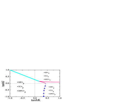
Figure 17: (Color online) Phase diagram of the AT model on the kaǵome lattice.

VII Acknowledgements

The work of Q.H.C was supported by National Basic Research Program of China (Grant Nos. 2011CBA00103 and 2009CB929104). The work of Y.D was supported by NSFC (Grant No. 10975127), Anhui Provincial Natural Science Foundation (Grant No. 090416224) and CAS.

References

- (1) C. Fan, Phys. Lett. 39A, 136(1972).
- (2) J. Ashkin, E. Teller, Phys. Rev. 64, 178 (1943).
- (3) J. X. Le and Z. R. Yang, Phys. Rev. E 68, 066105 (2003); Phys. Rev. E 69, 066107(2004).
- (4) A. Giuliani, V. Mastropietro, Phys. Rev. Lett. 93, 190603(2004).
- (5) C. Naón, Phys. Rev. E 79, 051112 (2009).
- (6) J. Salas, A. D. Sokal, J. Stat. Phys. 85, 297(1996).
- (7) F. Iglói and J. Zittartz, Z. Phys. B 73,125(1988).
- (8) P. Bak, P. Kleban, W. N. Unertl, J. Ochab, G. Akinci, N. C. Bartelt, T. L. Einstein, Phys. Rev. Lett. 54, 1539(1985).
- (9) E. Domany, E. K. Riedel, Phys. Rev. Lett. 40, 561(1978).
- (10) N. C. Bartelt, T. L. Einstein, L. T. Wille, Phys. Rev. B 40, 10759 (1989).
- (11) H. N. V. Temperley and S. E. Ashley, Proc. R. Soc. London A 365, 371 (1979).
- (12) Y. Deng, J. Salas, and A. D. Sokal, unpublished.
- (13) H. T. Diep and H. Giacomini, Chapter “Exactly Solved Frustrated Models” in Book “Frustrated Spin Systems”, World Scientific, 2005.
- (14) G. H. Wannier, Phys. Rev. 79, 357(1950); Phys. Rev. B 7, 5017(E)(1973).
- (15) J. Stephenson, J. Math. Phys. 11, 413 (1970).
- (16) R. H. Swendsen and J. S. Wang, Phys. Rev. Lett. 58, 86(1987).
- (17) G. M. Zhang, C. Z. Yang, Phys. Rev. B 50,12546 (1994).
- (18) P. D. Coddington, L. Han, Phys. Rev. B 50, 3058(1994).
- (19) W. Zhang, T.M. Garoni, Y. Deng, Nucl. Phys. B 814, 461(2009).
- (20) Q. Q. Liu, Y. Deng, and T. M. Garoni, Nucl. Phys. B 846, 238(2011), and references therein.
- (21) N. Prokof’ev, B. Svistunov, Phys. Rev. Lett. 87, 160601 (2001).
- (22) Y. Deng, T. M. Garoni, A. D. Sokal, Phys. Rev. Lett. 99, 110601(2007).
- (23) B. Nienhuis, Phys. Rev. Lett. 49, 1062(1982).
- (24) U. Wolff, Nucl. Phys. B 824, 254 (2009). See also in arxiv:1009.0657, and references therein.
- (25) K. Binder, Z. Phys. B 43, 119(1981).
- (26) Y. Deng, H. W. J. Blöte, Phys. Rev. E 68, 036125(2003).
- (27) G. Kamieniarz and H. W. J. Blöte, J. Phys. A: Math. Gen. 26, 201(1993).
- (28) Y. Deng, T. M. Garoni, W. Guo, H. W. J. Blöte, and Alan D. Sokal, Phys. Rev. Lett. 98, 120601(2007).
- (29) H. W. J. Blöte, M. P. Nightingale, Phys. Rev. B47, 15046(1993); H. W. J. Blöte, M. P. Nightingale, X. N. Wu, and A. Hoogland, Phys. Rev. B43, 8751(1991); X. Qian, M. Wegewijs, and H. W. J. Blöte, Phys. Rev. E 69, 036127 (2004).
- (30) A. D. Sokal, Monte Carlo methods in statistical mechanics: Foundations and new algorithms, in: P. C. C. DeWitt-Morette, A. Folacci (Eds.), Functional Integration: Basics and Applications, Plenum, New York, 1997, pp. 131–192.