Purification of noisy quantum measurements

Abstract

We consider the problem of improving noisy quantum measurements by suitable preprocessing strategies making many noisy detectors equivalent to a single ideal detector. For observables pertaining to finite-dimensional systems (e.g. qubits or spins) we consider preprocessing strategies that are reminiscent of quantum error correction procedures and allows one to perfectly measure an observable on a single quantum system for increasing number of inefficient detectors. For measurements of observables with unbounded spectrum (e.g. photon number, homodyne and heterodyne detection), the purification of noisy quantum measurements can be achieved by preamplification as suggested by H. P. Yuen yuen .

I Introduction

In many situations it is necessary to measure an observable in the presence of noise, e.g. when transmitting a quantum state through a noisy quantum channel that degrades it exponentially versus distance, corresponding to a degradation of the measurement.

A number of figures of merit can be used to characterize the noise of non-ideal measurements. An example of such figures of merit is the variance of the outcomes distribution. An extensive analysis of the variance affecting quantum measurements has been done for example in ozawa . In a communication scenario, a relevant figure of merit is represented by the mutual information between the measurement outcomes and the input alphabet encoded on an ensemble of states. The problem of how much classical information can be extracted from a quantum system has been first deeply discussed by Holevo holevo , who provided bounds on the accessible information, and then revisited in the framework of quantum information by Schumacher et al.schumacher . A further figure of merit is the average probability of correctly distinguishing input states picked up from a given ensemble. This is one of the first problems faced by quantum estimation theory, and has been addressed extensively in the literature holevo ; hel ; fuchs ; buscemi06 . Finally, another example of figure of merit is a suitable distance between the noisy and the ideal outcomes probability for fixed input states.

In this paper, we consider the situation where $N$ identical preparations of the state $\rho_{g}$ belonging to some ensemble $\mathcal{S}=\{(p_{g},\rho_{g})\}$ are given. We are allowed to use $M$ non-ideal detectors, with $M\geq N$. Each detector is described by a Probability Operator-Valued Measure (POVM), namely a set of positive operators $\{P^{\prime}_{i}\}$, which provides a resolution of the identity, i.e. $\sum_{i}P^{\prime}_{i}=I$. Each POVM element $P^{\prime}_{i}$ is the noisy version of an ideal POVM element $P_{i}$. A generic quantum channel $\mathcal{R}$ is allowed to act on the $N$ identical copies of the state $\rho_{g}$ before the $M$ noisy POVM $\{P^{\prime}_{i}\}$ are measured, and a generic classical post-processing can be done on the outcomes of such measurements. Such a scheme of “purification” of noisy measurements is depicted in Fig. 1.

Figure 1: Purification scheme for noisy quantum measurements.

We address the problem of optimizing the quantum channel $\mathcal{R}$ in order to reduce the effect of noise affecting the POVMs $\{P^{\prime}_{i}\}$. We approach the problem through the minimization of the variance of the maximum likelihood estimator for the parameter $g$ and through the maximization of the mutual information between $g$ and the measurement outcomes.

Notice the analogy between quantum error correction schemes gottesman , as depicted in Fig. 2, and the purification of measurements.

Figure 2: Scheme for quantum error correction.

For error correction, the message is first encoded by gate $\mathcal{R}$ into one of the carefully chosen codewords, which is then (possibly) corrupted by the noisy communication channel $\mathcal{E}$. Finally, in gate $\mathcal{D}$ some set of commuting Hermitian operators are measured over the corruption, the syndrome is used to perform error correction, and finally the recovered codeword is decoded into the original message. For purification of measurements, we are allowed to encode the $N$ identical copies of input state $\rho_{g}$ through the channel $\mathcal{R}$, in a way similar to quantum error correction. The aim of such encoding is very different, since after that we are forced to perform $M$ measurements with the same noisy POVM $\{P^{\prime}_{i}\}$, which provide us just classical outcomes to be classically post-processed. The limitation of the measurement purification versus error correction is that the decoding $\mathcal{D}$ is restricted to classical outcomes only. The problem we are considering is also similar to the problem solved by entanglement purification protocols bennet , since we are generally trying to recast the use of a number of noisy measurements to an effective use of a smaller number with less noise.

The paper is organized as follows. In Sect. II we specify the general problem to a qubit with isotropic noise, and then we face the optimization considering different figures of merit: in Sect. III we show how to minimize the measurement noise, while in Sect. IV we maximize the mutual information between the parameter describing the state and the outcomes of the POVMs. In Sect. V and Sect. VI, we consider observables with unbounded spectrum, for which the concept of amplification applies, and we review the scheme of H. P. Yuen yuen for purifying photodetectors (Sect. V), homodyne and heterodyne detectors (Sect. VI). Finally, Sect. VII is devoted to conclusions.

II Purification of Qubit Measurements

Let us specify the general problem we are considering. We are provided with $N$ identical copies of the input state $\rho_{g}$ of dimension $d$. In what follows we will always suppose that the elements of the POVMs $\{P_{i}\}$ and $\{P^{\prime}_{i}\}$ are $d$, which has been proved to be the optimal choice for $d=2$ levitin , when the mutual information is optimized . We suppose that each noisy element $P^{\prime}_{i}$ is obtained acting with the same channel $\mathcal{E}$ on the corresponding element $P_{i}$ of the ideal POVM

$$P^{\prime}_{i}=\mathcal{E}^{\vee}(P_{i}),$$ (1)

where $\mathcal{E}^{\vee}$ denotes the Heisenberg-picture version of the channel $\mathcal{E}$. Eq. (1) shows that the ideal POVM $\{P_{i}\}$ is “cleaner” that the noisy POVM $\{P^{\prime}_{i}\}$ in the sense of the partial ordering introduced in buscemi05 , as depicted in Fig. 3.

Figure 3: Noisy POVM element.

We consider a qubit (so $d=2$) parametrized as

$$\rho_{a,b}=\left(\begin{array}[]{cc}a&b\\ b^{*}&1-a\end{array}\right).$$ (2)

We are interested in the observable $\sigma_{z}$, and we suppose to have at our disposal $M$ noisy POVM $\{P^{\prime}_{i}\}$ of $\sigma_{z}$, i.e. $P_{i}=|i\rangle\langle i|$. We assume a simple kind of noise acting on each POVM, i.e. the isotropic noise

$$\mathcal{E}^{\vee}(P_{i})=\alpha P_{i}+\beta I,$$ (3)

so that $P^{\prime}_{i}=\alpha|i\rangle\langle i|+\beta I$.

We suppose to have $N=1$ qubit state and consider as a purification channel $\cal{R}$ the orthogonal cloning $\mathcal{C}$, with respect to the basis of eigenstates of the observable $\sigma_{z}$

$$\mathcal{C}(\rho)=\sum_{i=0,1}\langle i|\rho|i\rangle|i\rangle\langle i|^{\otimes M}.$$ (4)

The conditional probability $p(\vec{\imath}|a,b)$ of obtaining outcomes $\vec{\imath}=\{i_{1},\dots,i_{M}\}$ given the state parametrized by $a$, $b$ does not depend on $b$, and can be explicitly written as

$$p(\vec{\imath}|a)=\operatorname{Tr}[\mathcal{C}(\rho)\mathcal{E}^{\vee}(P_{i})^{\otimes M}]\;.$$ (5)

We substitute Eq. (4) and Eq. (3) into Eq. (5) to obtain

$$p(\vec{\imath}|a)=\operatorname{Tr}[(a|0\rangle\langle 0|^{\otimes M}+(1-a)|1\rangle\langle 1|^{\otimes M})\otimes_{j=1}^{M}(\alpha|i_{j}\rangle\langle i_{j}|+\beta I)]$$ (6)

We observe that the probability $p(\vec{\imath}|a)$ depends only on the number of outcomes $0$’s and $1$’s in the measurement (i.e., not on their position). Upon defining such integers as $M_{0}$ and $M_{1}=M-M_{0}$, we obtain

$$p(M_{1}|a)={M\choose M_{1}}\left[a(\alpha+\beta)^{M_{0}}\beta^{M_{1}}+(1-a)(\alpha+\beta)^{M_{1}}\beta^{M_{0}}\right]\;.$$ (7)

For the normalization condition of the POVM in Eq. (3) one has $\alpha=1-2\beta$, so $0\leq\beta\leq\frac{1}{2}$, and hence

$$p(M_{1}|a)={M\choose M_{1}}\left[a\left((1-\beta)^{M_{0}}\beta^{M_{1}}-(1-\beta)^{M_{1}}\beta^{M_{0}}\right)+(1-\beta)^{M_{1}}\beta^{M_{0}}\right]\,.$$ (8)

One can easily check the normalization of this probability, i.e. $\sum_{M_{1}=0}^{M}p(M_{1}|a)=1$. In the case of ideal measurements for which $\beta=0$, the non-null probabilities are obtained just for $M_{1}=0$ and for $M_{1}=M$, namely

$$p(M_{1}=0|a)=a,\qquad p(M_{1}=M|a)=1-a,$$ (9)

whereas in the completely isotropic case (i.e. $\beta=\frac{1}{2}$) the probability $p(M_{1}|a)={M\choose M_{1}}\left(\frac{1}{2}\right)^{M}$ is independent of $a$, namely no information can be obtained about the state.

Notice that also the coherent channel, widely used in encoding schemes for quantum error correction as shor95 ,

$$\mathcal{C}^{\prime}(\rho)=\sum_{i,j=0,1}\langle i|\rho|j\rangle|i\rangle\langle j|^{\otimes M}.$$ (10)

leads to the same probability distribution Eq. (8), since $P^{\prime}_{i}$ are diagonal on the $\sigma_{z}$ basis.

III Minimization of Measurement Noise

We show how to apply the ML criterion to obtain the optimal estimator for the expectation value of $\sigma_{z}$, by means of our measurement purification scheme. Our aim is to show an improvement of estimation in terms of variance by increasing the uses of the POVM. In the following $\log$ will denote the logarithm to the base $2$.

The ML criterion provides the following estimator for $a$ in the state Eq. (2)

$$a_{ML}=\operatorname{arg}\max_{a}\frac{1}{n}L(a|M_{1})$$ (11)

where $n$ is the number of (joint) outcomes (runs of the purification scheme depicted in Fig. 1), $L(a|M_{1})$ is the so called log-likelihood functional

$$L(a|M_{1})=\sum_{j=1}^{n}\log p_{j}(M_{1}|a),$$ (12)

and $p_{j}(M_{1}|a)$ denotes the conditional probability for the $j$-th run. We observe that Eq. (11) is concave since the logarithm of a linear function is a concave function and the summation of concave functions is a concave function.

To solve the ML problem, we employ the iterative numerical method described in rao . First, we generate a large amount of data distributed according to Eq. (8), for some fixed value of $a$ and $\beta$. Then, we fix some order zero approximation $a_{0}$ for the estimator $a_{ML}$. Then, the first order correction is given by

$$a_{1}=\frac{\left.\frac{\partial L(a|M_{1})}{\partial a}\right|_{a=a_{0}}}{F(a_{0})}$$ (13)

where $F(a)$ is the Fisher information

$$F(a)=\sum_{\vec{\imath}}\left(\frac{\partial{p(\vec{\imath}|a)}}{\partial{a}}\right)^{2}\frac{1}{p(\vec{\imath}|a)},$$ (14)

which in our case is given by

$$F(a)=\sum_{M_{1}=0}^{M}{M\choose M_{0}}^{2}\frac{\left((1-\beta)^{M_{0}}\beta^{M_{1}}-(1-\beta)^{M_{1}}\beta^{M_{0}}\right)^{2}}{p(M_{1}|a)}.$$ (15)

The Fisher information measures the amount of information that the random variable $M_{1}$ carries about the unknown parameter $a$ on which the likelihood function depends. So, the estimator to first order is $a_{0}+a_{1}$, and the procedure can be iterated with this value as order zero approximation to obtain higher order corrections. Obviously, the result is independent of the initial value $a_{0}$. For $\beta$ not too big (say $0<\beta<\frac{1}{3}$), the algorithm converges in a few steps (say, less than $10$).

The variance on the ML estimator of a parameter satisfies the Cramer-Rao bound cramer

$$\sigma^{2}(a_{ML})\geq\frac{1}{nF(a)}$$ (16)

The bound in Eq. (16) is saturated if the number of data is large enough and the parameter is mono-dimensional (as in the present case). We numerically estimated the variance of the estimator $a_{ML}$ in Eq. (11) by dividing the data into blocks, finding the estimator $a_{i}$ for each block, and then calculating the variance of such estimators, namely

$$\sigma^{2}(a_{ML})=\sum_{i}(a_{i}-a_{ML})^{2}.$$ (17)

In Fig. 4 we verified that the variance numerically saturates the bound in Eq. (16).

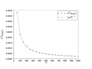
Figure 4: (Color online) Variance $\sigma^{2}(a_{ML})$ versus the number $n$ of outcomes (runs), for parameter $a=0.75$, measurement noise $\beta=0.25$, and number of POVMs $M=10$. The solid line represents the Cramer-Rao bound in Eq. (16).

Fig. 5 shows that the variance decreases as the number of POVMs used in parallel increases, and upper and lower bounds for variance.

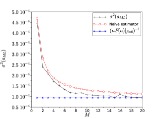
Figure 5: (Color online) Variance $\sigma^{2}(a_{ML})$ versus the number $M$ of POVMs, for parameter $a=0.75$, measurement noise $\beta=0.25$, and number of runs $n=2000$. The upper and lower bound correspond to Eqs. (21) and (22), respectively.

To find the upper bound consider the function

$$f(M_{1})=\frac{\frac{M_{1}}{M}+\beta-1}{2\beta-1}.$$ (18)

Notice that $f(M_{1})$ is an unbiased estimator for the parameter $a$, since one has

$$\langle f(M_{1})\rangle=\sum_{M_{1}=0}^{M}f(M_{1})p(M_{1}|a)=a.$$ (19)

The second moment is given by

$$\begin{split}\langle f(M_{1})^{2}\rangle&=\sum_{M_{1}=0}^{M}f(M_{1})^{2}p(M_{1}|a)\\ &=a+\frac{\beta(1-\beta)}{(1-2\beta)^{2}M}.\end{split}$$ (20)

Thus, an upper bound for the variance on the parameter $a$ is

$$\sigma^{2}(a_{ML})\leq\left(a-a^{2}+\frac{\beta(1-\beta)}{(1-2\beta)^{2}M}\right)\frac{1}{n}.$$ (21)

The lower bound for the variance is

$$\sigma^{2}(a_{ML})\geq\frac{1}{nF(a)|_{\beta=0,M=1}}=\frac{a-a^{2}}{n},$$ (22)

where the right-hand side of Eq. (22) corresponds to the use of the ideal detector on the original state.

The computed variance shows a dependence on the parameter $a$ similar that in Eq. (21), decreasing as $1/M$ for $a=0$ or $a=1$. The variance saturates the lower bound in Eq. (22), so the the estimator of the parameter $a$ is optimal.

IV Maximization of Mutual Information

We consider now the mutual information as the figure of merit in the measurement purification scheme. We consider a qubit parametrized as

$$|\psi\rangle=\cos{\frac{\theta}{2}}|0\rangle+e^{i\phi}\sin{\frac{\theta}{2}}|1\rangle.$$ (23)

The probability in Eq. (8) can be written as

$$p(M_{1}|\theta)={M\choose M_{1}}\left[[(1-\beta)^{M_{0}}\beta^{M_{1}}-(1-\beta)^{M_{1}}\beta^{M_{0}}]\cos^{2}{\frac{\theta}{2}}+(1-\beta)^{M_{1}}\beta^{M_{0}}\right],$$ (24)

independent of $\phi$.

In the following we suppose that the prior probability $p(\theta,\phi)$ of having the input state in Eq. (23) is uniform, so that the mutual information $I(M_{1}:\theta,\phi)$ between random variables $\theta$ and $\phi$ and random variable $M_{1}$ is given by

$$I(M_{1}:\theta):=\frac{1}{2}\int_{0}^{\pi}d\theta\sin\theta\sum_{M_{1}=0}^{M}p(M_{1}|\theta)\log\left(\frac{p(M_{1}|\theta)}{\frac{1}{2}\int_{0}^{\pi}d\theta\sin\theta p(M_{1}|\theta)}\right).$$ (25)

The integral in the denominator gives

$$\int_{0}^{\pi}d\theta\sin\theta p(M_{1}|\theta)={M\choose M_{1}}((1-\beta)^{M_{0}}\beta^{M_{1}}+(1-\beta)^{M_{1}}\beta^{M_{0}})\,,$$ (26)

and a lengthy analytical form for Eq. (25) is provided in the Appendix of the paper.

The mutual information $I(M_{1}:\theta)$ saturates the bound $I(M_{1}:\theta)\leq I(M_{1}:\theta)|_{M=1,\beta=0}\simeq 0.279\operatorname{bit}$ for increasing M. Notice that the mutual information does not converge to $1\operatorname{bit}$, since a continuous “alphabet” of states is allowed. The mutual information $I(M_{1}:\theta)$ saturates almost exponentially versus $M$, as shown by Fig. 6.

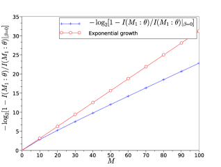
Figure 6: (Color online) Function $-\log_{2}\left[1-\frac{I(M_{1}:\theta)}{I(M_{1}:\theta)|_{\beta=0}}\right]$ versus the number $M$ of POVMs, for measurement noise $\beta=0.25$. The mutual information $I(M_{1}:\theta)$ is given by Eq. (78).

This means that we are recasting the use of many noisy detectors to an effective use of a single ideal detector.

Let us consider in more detail the simplified case in which the only allowed input state are the up ($\theta=\pi$) and down ($\theta=0$) eigenstates of $\sigma_{z}$. This simplification leads to two advantages: a much more tractable analytical form for the mutual information $I_{2}(M_{1}:\theta)$, and the possibility to make a comparison with classical post-processing based on majority voting. The mutual information is given by

$$I_{2}(M_{1}:\theta)=\sum_{M_{1}=0}^{M}{M\choose M_{1}}(1-\beta)^{M_{1}}\beta^{M_{0}}\log\left[\frac{2(1-\beta)^{M_{1}}\beta^{M_{0}}}{(1-\beta)^{M_{0}}\beta^{M_{1}}+(1-\beta)^{M_{1}}\beta^{M_{0}}}\right].$$ (27)

Eq. (27) behaves as expected for the ideal POVM case (i.e. $\beta=0$), where $I_{2}(M_{1}:\theta)=1$, and for completely isotropic POVM case (i.e. $\beta=\frac{1}{2}$) where $I_{2}(M_{1}:\theta)=0$. Finally, we investigate the optimal classical post-processing to be applied on the $M$ outcomes of the parallel noisy POVMs to maximize the mutual information. We simply argue that majority voting is close to the optimal post-processing, as is shown in plot Fig. 7.

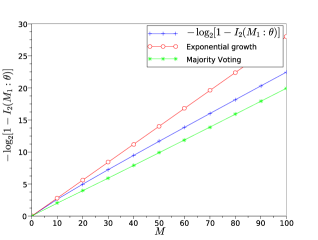
Figure 7: (Color online) Function $-\log_{2}[1-I_{2}(M_{1}:\theta)]$ versus the number $M$ of POVMs, for measurement noise $\beta=0.25$.

The gap between the binary mutual information $I_{2}(M_{1}:\theta)$ and that obtained with majority-voting strategy could be explained by the fact that in general a number of POVM elements greater than the cardinality of the input alphabet can optimize the mutual information. In fact, Davies’ theorem davies puts an upper bound of $d^{2}$ on the number of POVM elements to optimize the mutual information for an alphabet of $d$ linear independent pure states (see also shor ).

The case of two-states alphabet can be easily generalized to an alphabet of $d$ orthogonal state $\{|j\rangle\}$, with $j=1,2,\ldots d$, and noisy POVM elements $P^{\prime}_{i}=\alpha|i\rangle\langle i|+\frac{1-\alpha}{d}I$. The conditional probability of the outcomes of $M$ noisy measurements on $M$ copies of $|j\rangle$ is simply the multinomial

$$p(M_{1},M_{2},\ldots,M_{d-1}|j)=\frac{M!}{M_{1}!M_{2}!\cdots M_{d}}\frac{[(d-1)\alpha+1]^{M_{j}}(1-\alpha)^{M-M_{j}}}{d^{M}}\;,$$ (28)

where $M_{l}$ is the number of outcomes $l$ in the string of $M$ outcomes, and $M_{d}=M-\sum_{j=1}^{d-1}M_{j}$. The conditional probability allows one to evaluate the mutual information, and for increasing number of clones $M$, the noisy measurements are purified. In Fig. 8 we show the purification effect for an alphabet of four orthogonal equiprobable states, and two different values of noise. As expected, for increasing value of $M$ the mutual information approaches two bits.

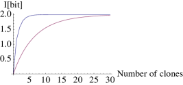
Figure 8: (Color online) Mutual information for an alphabet of four equiprobable orthogonal states versus number of purifying copies, for measurement noise $\alpha=0.8$ (upper), and $\alpha=0.4$ (lower).

V Inefficient photodetection

In the rest of the paper we consider observables with unbounded spectrum, for which the concept of amplification applies, and we review the scheme of H. P. Yuen yuen for improving noisy photodetectors, homodyne and heterodyne detectors. In the original proposal of Ref. yuen the signal-to-noise ratio improvement was studied for noisy measurements with preamplification assistance. By reviewing the results here, we explicitly consider the effect of amplification as a purification of the noisy POVMs, and hence of the outcome probability distributions.

Light is revealed by exploiting its interaction with atoms/molecules or electrons in a solid, and, essentially, each photon ionizes a single atom or promotes an electron to a conduction band, and the resulting charge is then amplified to produce a measurable pulse. In practice, however, available photodetectors are not ideally counting all photons, and their performances is limited by a non-unit quantum efficiency $\eta$, namely only a fraction $\eta$ of the incoming photons lead to an electric signal, and ultimately to a count: some photons are either reflected from the surface of the detector, or are absorbed without being transformed into electric pulses. Let us consider a light beam entering a photodetector of quantum efficiency $\eta$, i.e. a detector that transforms just a fraction $\eta$ of the incoming light pulse into electric signal. We will focus our attention to the case of the radiation field excited in a stationary state of a single mode at frequency $\omega$. Then, the Poissonian process of counting gives the following probability $p_{\eta}(m)$ of revealing $m$ photons kelley

$$p_{\eta}(m)=\hbox{Tr}\left[\rho\,\mbox{{\bf:}}{\frac{(\eta a^{{\dagger}}a)^{m}}{m!}}\exp(-\eta a^{{\dagger}}a)\mbox{{\bf:}}\right]\;,$$ (29)

where $\rho$ represents the quantum state of light, and :  : denotes the normal ordering of field operators.

Using the identities

$$\mbox{{\bf:}}({a^{\dagger}}a)^{n}\mbox{{\bf:}}=({a^{\dagger}})^{n}a^{n}={a^{\dagger}}a({a^{\dagger}}a-1)\ldots({a^{\dagger}}a-n+1)\;,$$ (30)

$$\mbox{{\bf:}}e^{-x{a^{\dagger}}a}\mbox{{\bf:}}=\sum_{l=0}^{\infty}{\frac{(-x)^{l}}{l!}}({a^{\dagger}})^{l}a^{l}=(1-x)^{{a^{\dagger}}a},$$ (31)

one obtains

$$p_{\eta}(m)=\sum_{n=m}^{\infty}\rho_{nn}\left(\begin{array}[]{c}n\\ m\end{array}\right)\eta^{m}(1-\eta)^{n-m}\;,$$ (34)

where

$$\rho_{nn}\equiv\langle n|\rho|n\rangle=p_{\eta=1}(n)\;.$$ (35)

Hence, for unit quantum efficiency a photodetector measures the photon number distribution of the state, whereas for non unit quantum efficiency the output distribution of counts is given by a Bernoulli convolution of the ideal distribution.

The outcome distribution in Eq. (34) can be equivalently described by means of a simple model in which the realistic photodetector is replaced with an ideal photodetector preceded by a beam splitter of transmissivity $\tau\equiv\eta$. The reflected mode is absorbed, whereas the transmitted mode is photodetected with unit quantum efficiency. In order to obtain the probability of measuring $m$ clicks, notice that, apart from trivial phase changes, a beam splitter of transmissivity $\tau$ affects the unitary transformation of fields

$$\left(\begin{array}[]{c}c\\ d\end{array}\right)\equiv U_{\tau}^{\dagger}\left(\begin{array}[]{c}a\\ b\end{array}\right)U_{\tau}=\left(\begin{array}[]{cc}\sqrt{\tau}&-\sqrt{1-\tau}\\ \sqrt{1-\tau}&\sqrt{\tau}\end{array}\right)\left(\begin{array}[]{c}a\\ b\end{array}\right)\;,$$ (44)

where all field modes are considered at the same frequency. Hence, the output mode $c$ hitting the detector is given by the linear combination

$$c=\sqrt{\tau}a-\sqrt{1-\tau}b\;,$$ (45)

and the probability of counts reads

$$p_{\tau}(m) = \hbox{Tr}\left[U_{\tau}(\rho\otimes|0\rangle\langle 0|)U^{{\dagger}}_{\tau}|m\rangle\langle m|\otimes 1\right]$$ (48)

$$= \sum_{n=m}^{\infty}\rho_{nn}\left(\begin{array}[]{c}n\\ m\end{array}\right)(1-\tau)^{n-m}\tau^{m}\;.$$

Equation (34) is then reproduced for $\tau=\eta$. We conclude that a photodetector of quantum efficiency $\eta$ is equivalent to a perfect photodetector preceded by a beam splitter of transmissivity $\eta$ which accounts for the overall losses of the detection process. According to Eq. (34), the POVM describing the inefficient photodetector can be written as

$$\Pi_{\eta}(m)=\left(\begin{array}[]{c}a^{\dagger}a\\ m\end{array}\right)\eta^{m}(1-\eta)^{a^{\dagger}a-m}\;,$$ (51)

such that $p_{\eta}(m)=\operatorname{Tr}[\rho\Pi_{\eta}(m)]$. The random variable $m$, suitably rescaled by $\eta$, provides an estimator of the average photon number $\langle a^{\dagger}a\rangle=\operatorname{Tr}[\rho a^{\dagger}a]$, since one has

$$\sum_{m=0}^{\infty}\frac{m}{\eta}\Pi_{\eta}(m)=a^{\dagger}a\;.$$ (52)

In order to evaluate the second moment of the probability, one uses the identity

$$\sum_{m=0}^{\infty}\left(\frac{m}{\eta}\right)^{2}\Pi_{\eta}(m)=(a^{\dagger}a)^{2}+\frac{1-\eta}{\eta}a^{\dagger}a\;,$$ (53)

and hence the inefficient measurement is affected by the added noise $\frac{1-\eta}{\eta}\langle a^{\dagger}a\rangle$, with respect to the ideal intrinsic noise $\Delta(a^{\dagger}a)^{2}\equiv\langle(a^{\dagger}a)^{2}\rangle-\langle a^{\dagger}a\rangle^{2}$.

In the following we show that and ideal photon-number amplifier can arbitrarily reduce the added noise of the inefficient measurement for increasing gain. The ideal photon-number amplification map is given by pna11 ; pna2 ; pna3

$$a^{{\dagger}}a\longrightarrow\hat{V}^{{\dagger}}\,a^{{\dagger}}a\,\hat{V}=g\,a^{{\dagger}}a\;,$$ (54)

where $g$ is an integer, and $\hat{V}$ is the isometry

$$\hat{V}=\sum_{n=0}^{\infty}|gn\rangle\langle n|\;.$$ (55)

The preamplified POVM is simply given by

$$\Pi^{(g)}_{\eta}(m)=\left(\begin{array}[]{c}ga^{\dagger}a\\ m\end{array}\right)\eta^{m}(1-\eta)^{ga^{\dagger}a-m}\;.$$ (58)

The estimator of the average photon number is now $m/(g\eta)$, and the second moment is given by

$$\sum_{m=0}^{\infty}\left(\frac{m}{g\eta}\right)^{2}\Pi^{(g)}_{\eta}(m)=(a^{\dagger}a)^{2}+\frac{1-\eta}{g\eta}a^{\dagger}a\;.$$ (59)

Clearly, for $g\to\infty$, the added noise is completely removed for any value of the quantum efficiency $\eta$.

We notice that the ideal photon-number amplifier is so effective that indeed even a preamplified heterodyne detection provides the ideal photon number distribution for increasing gain, as shown in Ref. dys .

VI Inefficient continuous variable measurements

VI.1 Homodyne detection

The balanced homodyne detector provides the measurement of the quadrature of the field

$$X_{\varphi}=\frac{{a^{\dagger}}e^{i\varphi}+ae^{-i\varphi}}{2}\;$$ (60)

It was proposed by Yuen and Chan yuenchan , and subsequently experimentally demonstrated by Abbas, Chan and Yee abbas . The signal mode $a$ interferes with a strong laser beam mode $b$ in a balanced 50/50 beam splitter. The mode $b$ is the so-called the local oscillator (LO) mode of the detector. It operates at the same frequency of $a$, and is excited by the laser in a strong coherent state $|z\rangle$. Since in all experiments that use homodyne detectors the signal and the LO beams are generated by a common source, we assume that they have a fixed phase relation. In this case the LO phase provides a reference for the quadrature measurement, namely we identify the phase of the LO with the phase difference between the two modes. By tuning $\varphi=\operatorname{arg}z$ we can measure the quadrature $X_{\varphi}$ at arbitrary phase.

Behind the beam splitter, the two modes are detected by two identical photodetectors (usually linear avalanche photodiodes), and finally the difference of photocurrents at zero frequency is electronically processed. In the strong-LO limit $|z|\to\infty$, the homodyne detector is described by the POVM

$$\Pi(x)=\int_{-\infty}^{+\infty}{\frac{d\lambda}{2\pi}}\,\exp[i\lambda(X_{\varphi}-x)]=|x\rangle_{\varphi}{}_{\varphi}\langle x|\;,$$ (61)

namely the projector on the eigenstate of the quadrature $X_{\varphi}$ with eigenvalue $x$. In conclusion, the balanced homodyne detector achieves the ideal measurement of the quadrature $X_{\varphi}$ in the strong LO limit. In this limit, the probability distribution of the output photocurrent approaches exactly the probability distribution $p(x,\varphi)={}_{\varphi}\langle x|\rho|x\rangle_{\varphi}$ of the quadrature $X_{\varphi}$, and this for any state $\rho$ of the signal mode $a$.

It is easy to take into account non-unit quantum efficiency at detectors. The POVM is obtained by replacing

$$X_{\varphi}\rightarrow X_{\varphi}+\sqrt{\frac{1-\eta}{2\eta}}(u_{\varphi}+v_{\varphi})\;$$ (62)

in Eq. (61), with $w_{\varphi}=(w^{\dagger}e^{i\varphi}+we^{-i\varphi})/2$, where $w=u,v$ denotes the vacuum modes of the two inefficient photodetectors. By tracing the vacuum modes $u$ and $v$, one obtains

$$\Pi_{\eta}(x) = \int_{-\infty}^{+\infty}\frac{d\lambda}{2\pi}\,e^{i\lambda(X_{\varphi}-x)}|\langle 0|e^{i\lambda\sqrt{\frac{1-\eta}{2\eta}}u_{\varphi}}|0\rangle|^{2}$$

$$= \int_{-\infty}^{+\infty}\frac{d\lambda}{2\pi}\,e^{i\lambda(X_{\varphi}-x)}e^{-\lambda^{2}\frac{1-\eta}{8\eta}}$$

$$= \frac{1}{\sqrt{2\pi\Delta^{2}_{\eta}}}\exp\left[-\frac{(x-X_{\varphi})^{2}}{2\Delta_{\eta}^{2}}\right]$$

$$= \frac{1}{\sqrt{2\pi\Delta^{2}_{\eta}}}\int_{-\infty}^{+\infty}dx^{\prime}\,e^{-\frac{1}{2\Delta_{\eta}^{2}}(x-x^{\prime})^{2}}\,|x^{\prime}\rangle_{\varphi}{}_{\varphi}\langle x^{\prime}|\;,$$

where

$$\Delta_{\eta}^{2}=\frac{1-\eta}{4\eta}\;.$$ (64)

Thus the noisy POVM, and in turn the probability distribution of the output photocurrent, are just the Gaussian convolution of the ideal ones with r.m.s. $\Delta_{\eta}=\sqrt{(1-\eta)/(4\eta)}$.

In the following we show that the added noise of the inefficient homodyne detector can be removed by amplifying the signal by means of a phase-sensitive amplifier. This amplifier is described by the squeezing operator

$$S(\xi)=\exp\left[\frac{1}{2}\left(\xi a^{{\dagger}2}-\xi^{*}a^{2}\right)\right]\;,$$ (65)

and performs the mode transformation

$$S^{\dagger}(\xi)aS(\xi)=(\cosh|\xi|)a+\frac{\xi}{|\xi|}(\sinh|\xi|)a^{\dagger}\;.$$ (66)

For $\xi=re^{2i\varphi}$, with $r>0$, one has

$$S^{\dagger}(\xi)X_{\varphi}S(\xi)=e^{r}X_{\varphi}\;.$$ (67)

Hence, the effective POVM obtained by preprocessing $\Pi_{\eta}(x)$ in Eq. (VI.1) with the phase-sensitive amplification of $X_{\varphi}$ is given by

$$\Pi^{(r)}_{\eta}(x) = S^{\dagger}(re^{2i\varphi})\Pi_{\eta}(x)S(re^{2i\varphi})$$ (68)

$$= \frac{1}{\sqrt{2\pi\Delta^{2}_{\eta}}}\exp\left[-\frac{(x-e^{r}X_{\varphi})^{2}}{2\Delta_{\eta}^{2}}\right]\;.$$

Now, in order to obtain an unbiased measurement of $X_{\varphi}$, it is enough to rescale the outcome by $e^{r}$. On the other hand, the added noise with respect to the ideal measurement $X_{\varphi}$ becomes equal to $e^{-2r}\Delta^{2}_{\eta}$, which can be made arbitrary small for increasing value of the squeezing parameter $r$.

VI.2 Heterodyne detection

Heterodyne detection allows to perform the joint measurement of two conjugated quadratures of the field hetyuen1 ; hetyuen2 .

A strong local oscillator at frequency $\omega$ in a coherent state $|\alpha\rangle$ hits a beam splitter with transmissivity $\tau\to 1$, and with the coherent amplitude $\alpha$ such that $\gamma\equiv|\alpha|\sqrt{\tau(1-\tau)}$ is kept constant. If the output photocurrent is sampled at the intermediate frequency $\omega_{IF}$, just the field modes $a$ and $b$ at frequency $\omega\pm\omega_{IF}$ are selected by the detector. Modes $a$ and $b$ are usually referred to as signal band and image band modes, respectively. In the strong LO limit, upon tracing the LO mode, the output photocurrent $I(\omega_{IF})$ rescaled by $\gamma$ is equivalent to the complex operator

$$Z=\frac{I(\omega_{IF})}{\gamma}=a-b^{\dagger},$$ (69)

where the arbitrary phases of modes have been suitably chosen. The heterodyne photocurrent $Z$ is a normal operator, equivalent to a couple of commuting self-adjoint operators

$$Z=\hbox{Re}Z+i\hbox{Im}Z\;,\qquad[Z,Z^{\dagger}]=[\hbox{Re}Z,\hbox{Im}Z]=0\;.\;$$ (70)

The POVM of the detector is then given by the orthogonal (in Dirac sense) eigenvectors of $Z$.

In conventional heterodyne detection the image band mode is in the vacuum state, and one is just interested in measuring the field mode $a$. In this case the POVM $\Pi(z)$ is obtained upon tracing on mode $b$, and one has the customary projectors on coherent states

$$\Pi(z)=\frac{1}{\pi}|z\rangle\langle z|\;,$$ (71)

with $z\in{\mathbb{C}}$. The coherent-state POVM provides the optimal joint measurement of conjugated quadratures of the field hel . For a state $\rho$, the expectation value of any quadrature $X_{\varphi}$ is obtained as

$$\langle X_{\varphi}\rangle=\hbox{Tr}[\rho X_{\varphi}]=\int_{\mathbb{C}}\frac{d^{2}\alpha}{\pi}\hbox{Re}(\alpha e^{-i\varphi})\langle\alpha|\rho|\alpha\rangle\;.$$ (72)

The price to pay for jointly measuring non-commuting observables is an additional noise. The r.m.s. fluctuation is evaluated as follows

$$\int_{\mathbb{C}}\frac{d^{2}\alpha}{\pi}[\hbox{Re}(\alpha e^{-i\varphi})]^{2}\langle\alpha|\rho|\alpha\rangle-\langle X_{\varphi}\rangle^{2}=\langle\Delta X^{2}_{\varphi}\rangle+\frac{1}{4}\;,$$ (73)

where $\langle\Delta X^{2}_{\varphi}\rangle$ is the intrinsic noise, and the additional term is usually referred to as “the additional 3dB noise due to the joint measure” Arthurs ; yuen82 ; goodman .

The effect of non-unit quantum efficiency can be taken into account in analogous way as in Sec. VI.1 for homodyne detection. The coherent-state POVM is replaced with the convolution

$$\Pi_{\eta}(z)=\int_{\mathbb{C}}\frac{d^{2}z^{\prime}}{\pi\Delta^{2}_{\eta}}e^{-\frac{|z^{\prime}-z|^{2}}{\Delta^{2}_{\eta}}}\frac{|z^{\prime}\rangle\langle z^{\prime}|}{\pi}\;,$$ (74)

where $\Delta^{2}_{\eta}=(1-\eta)/\eta$.

In the following we show that inefficient heterodyne detection can be purified by phase-insensitive amplification. Phase-insensitive amplification with (power) gain G amplifies the coherent amplitude of coherent states by $\sqrt{G}$, at the expense of addition thermal photons $\bar{n}=G-1$. Differently from phase-insensitive amplification, the physical process is not unitary, but described by a completely positive map ${\cal E}_{G}$. Here, we just need the Heisenberg evolution of the projector on coherent states, which is simply given by the rescaling caves

$${\cal E}_{G}^{\vee}(|\alpha\rangle\langle\alpha|)=\frac{1}{G}|G^{-1/2}\alpha\rangle\langle G^{-1/2}\alpha|\;.$$ (75)

It follows that under phase-insensitive preamplification the noisy heterodyne POVM (74) is replaced with

$$\Pi^{(G)}_{\eta}(z)=\int_{\mathbb{C}}\frac{d^{2}z^{\prime}}{\pi\Delta^{2}_{\eta}}e^{-\frac{|\sqrt{G}z^{\prime}-z|^{2}}{\Delta^{2}_{\eta}}}\frac{|z^{\prime}\rangle\langle z^{\prime}|}{\pi}\;.$$ (76)

Upon rescaling $z\to G^{-1/2}z$, one obtains

$$\Pi^{(G)}_{\eta}(z) =\int_{\mathbb{C}}\frac{Gd^{2}z^{\prime}}{\pi\Delta^{2}_{\eta}}e^{-\frac{G|z^{\prime}-z|^{2}}{\Delta^{2}_{\eta}}}\frac{|z^{\prime}\rangle\langle z^{\prime}|}{\pi}\;$$ (77)

$$=_{\scriptsize{G\to\infty}}\frac{|z\rangle\langle z|}{\pi}\;,$$

namely the noise due to quantum efficiency can be arbitrarily reduced for increasing value of the gain $G$. The effectiveness of preamplification in purifying heterodyne detection is more unexpected than the case of homodyne detection, since phase-insensitive amplification is not a unitary process.

VII Conclusion

In this paper, we addressed the problem of optimizing a quantum channel acting before many parallel uses of a noisy POVM in order to purify the measurements, namely to achieve an effective measurement that is less noisy than the original ones. We first considered the purification of $\sigma_{z}$ noisy measurements on qubits, by choosing the orthogonal cloning channel as a purification map. We found the maximum-likelihood estimator for $\sigma_{z}$, whose variance shows an almost-exponential decay of versus the number of POVMs. We also worked out an analytic form for the mutual information between the state parameter and the outcomes of the POVMs, and here also an almost-exponential improvement versus the number of POVMs has been found. We proved that naive majority voting is not the optimal classical post-processing, since the maximum-likelihood approach gives a better estimator. For photodetection and continuous variable measurements as homodyne and heterodyne detection, the measurement purification can be achieved by preamplification, as early pointed out by H. P. Yuen yuen .

We think that the relevant problem of purifying noisy quantum measurements will have a significant impact on the quantum information technology, in this same way as the decoherence problem.

Acknowlegments

This work is supported by Italian Ministry of Education through PRIN 2008 and the European Community through COQUIT project.

Appendix A Derivation of the mutual information in Eq. (25)

We provide here an analytic form for Eq. (25), obtained substituting Eq. (8) for $p(M_{1}|\theta)$. One obtains

$$I(M_{1}:\theta)=\frac{1}{32}\sum_{M_{1}=0}^{M}{M\choose M_{1}}\frac{c_{1}A+c_{2}B}{C},$$ (78)

where

$$c_{1}=(1-\beta)^{2M}\beta^{4M_{1}},\qquad c_{2}=(1-\beta)^{4M_{1}}\beta^{2M},$$ (79)

and

$$\begin{split}A=&-16\log((1-\beta)^{2M_{1}}\beta^{M}+(1-\beta)^{M}\beta^{2M_{1}})\\ &+8\log((1-\beta)^{2M}\beta^{4M_{1}})+16-8\frac{1}{\ln(2)},\end{split}$$ (80)

$$\begin{split}B=&+16\log((1-\beta)^{2M_{1}}\beta^{M}+(1-\beta)^{M}\beta^{2M_{1}})\\ &-8\log((1-\beta)^{4M_{1}}\beta^{2M})-16+8\frac{1}{\ln(2)},\end{split}$$ (81)

$$C=(1-\beta)^{M+M_{1}}\beta^{3M_{1}}-(1-\beta)^{3M_{1}}\beta^{M+M_{1}}.$$ (82)

References

- (1) H. P. Yuen, Opt. Lett. 12, 789 (1987).
- (2) M. Ozawa, Ann. Phys. 311, 350 (2004).
- (3) A. S. Holevo, Problems Inform. Transmission 9, 110 (1973).
- (4) B. Schumacher, M. Westmoreland, and W. K. Wootters, Phys. Rev. Lett. 76, 3452 (1996).
- (5) C. W. Helstrom, Quantum Detection and Estimation Theory (Academic Press, New York, 1976).
- (6) C. A. Fuchs, arXiv:quant-ph/9601020v1.
- (7) F. Buscemi and M. F. Sacchi, Phys. Rev. A 74, 052320 (2006).
- (8) D. Gottesman, arXiv:quant-ph/0904.2557v1.
- (9) C. H. Bennett, G. Brassard, S. Popescu, B. Schumacher, J. A. Smolin, and W. K. Wootters, Phys. Rev. Lett. 76, 722 (1996).
- (10) L. B. Levitin, in Quantum Communications and Measurement, ed. by V. P. Belavkin, O. Hirota and R. L. Hudson (Plenum Press, New York, 1995), p. 439; A. Keil, arXiv:quant-ph/0809.0232.
- (11) P. W. Shor, in Quantum Communication, Computing, and Measurement 3, ed. by P. Tombesi and O. Hirota (Kluwer, New York, 2001), p. 107.
- (12) F. Buscemi, G. M. D’Ariano, M. Keyl, P. Perinotti, and R. Werner, J. Math. Phys. 46, 082109 (2005).
- (13) P. W. Shor, Phys. Rev. A 52, 2493 (1995).
- (14) C. R. Rao, Linear Statistical Inference and Its Applications (John Wiley & Sons, New York, 1976).
- (15) H. Cramer, Mathematical Methods of Statistics (Princeton Univ. Press., Princeton, 1946).
- (16) E. B. Davies, IEEE Inf. Theory 24, 596 (1978).
- (17) P. L. Kelley and W. H. Kleiner, Phys. Rev. 136, A316 (1964).
- (18) H. P. Yuen, Phys. Lett. A 113, 405 (1986).
- (19) G. M. D’Ariano, Phys. Rev. A 45, 3224 (1992).
- (20) G. M. D’Ariano, C. Macchiavello, N. Sterpi, and H. P. Yuen, Phys. Rev. A 54, 4712 (1996).
- (21) G. M. D’Ariano, M. F. Sacchi, and H. P. Yuen, Int. J. Mod. Phys. B 13, 3069 (1999).
- (22) H. P. Yuen and V. W. S. Chan, Opt. Lett. 8, 177 (1983).
- (23) G. L. Abbas, V. W. S. Chan, S. T. Yee, Opt. Lett. 8, 419 (1983); IEEE J. Light. Tech. LT-3, 1110 (1985).
- (24) H. P. Yuen and J. H. Shapiro, IEEE Trans. Inf. Theory 24, 657 (1978); 25, 179 (1979).
- (25) H. P. Yuen and J. H. Shapiro, IEEE Trans. Inf. Theory 26, 78 (1980).
- (26) E. Arthurs and J. L. Kelly, Jr., Bell System Tech. J. 44, 725 (1965).
- (27) H. P. Yuen, Phys. Lett. 91A, 101 (1982).
- (28) E. Arthurs and M. S. Goodman, Phys. Rev. Lett. 60, 2447 (1988).
- (29) C. M. Caves and P. D. Drummond, Rev. Mod. Phys. 66, 481 (1994).